UCRL-JRNL-226480

No-core shell model for $A=47$ and $A=49$

Abstract

We apply the no-core shell model to the nuclear structure of odd-mass nuclei straddling ⁴⁸Ca. Starting with the NN interaction, that fits two-body scattering and bound state data we evaluate the nuclear properties of $A=47$ and $A=49$ nuclei while preserving all the underlying symmetries. Due to model space limitations and the absence of 3-body interactions, we incorporate phenomenological interaction terms determined by fits to $A=48$ nuclei in a previous effort. Our modified Hamiltonian produces reasonable spectra for these odd mass nuclei. In addition to the differences in single-particle basis states, the absence of a single-particle Hamiltonian in our no-core approach complicates comparisons with valence effective NN interactions. We focus on purely off-diagonal two-body matrix elements since they are not affected by ambiguities in the different roles for one-body potentials and we compare selected sets of $fp$-shell matrix elements of our initial and modified Hamiltonians in the harmonic oscillator basis with those of a recent model $fp$-shell interaction, the GXPF1 interaction of Honma, Otsuka, Brown and Mizusaki. While some significant differences emerge from these comparisons, there is an overall reasonably good correlation between our off-diagonal matrix elements and those of GXPF1.

I Introduction

The low-lying levels of the $A=47-49$ nuclei have long been of experimental and theoretical interest. On the one hand, extensive experimental information about these nuclei is available [BUR95] -[ENDS] and, on the other hand, this is a suitable nuclear mass region for developing and testing effective $fp$-shell Hamiltonians. Numerous detailed spectroscopic calculations have been reported. For example, in Ref. [MZPC96] , using a shell model approach, Martinez-Pinedo, Zuker, Poves and Caurier have performed full $fp$-shell calculations for the $A=47$ and $A=49$ isotopes of Ca, Sc, Ti, V, Cr and Mn. They employed the KB3 interaction [KB3] with phenomenological adjustments and they performed complete diagonalizations to obtain very good agreement with the experimental level schemes, transition rates and static moments. Extensive discussions of $fp$-shell effective Hamiltonians and nuclear properties can be found in recent shell model review articles [BAB01] ; [OtsukaHMSU01] ; [DJDean04] ; [Caurier05] .

Our interest in these nuclei stems from our goal to extend the no-core shell model (NCSM) applications to heavier systems than previously investigated. Until recently, the NCSM, which treats all nucleons on an equal footing, had been limited to nuclei up through $A=16$. However, in a recent paper [VPSN06] we reported the first NCSM results for ⁴⁸Ca, ⁴⁸Sc and ⁴⁸Ti isotopes, with derived and phenomenological two-body Hamiltonians. These three nuclei are involved in double-beta decay of ⁴⁸Ca, and the interest in developing nuclear structure models for describing them is also related to the need for accurate calculations of the nuclear matrix elements involved in this decay. Our first goals were to see the limitations of such an approach applied to heavier systems and how much improvement one can obtain by adding phenomenological two-body terms involving all nucleons. In brief, the results were the following [VPSN06] : i) one finds that the charge dependence of the bulk binding energy of eight $A=48$ nuclei is reasonably described with an effective Hamiltonian derived from CD-Bonn interactionMachl in the very limited $N_{\rm max}=0$ basis space, while there is an overall underbinding by about $0.4$ MeV/nucleon; ii) the resulting spectra are too compressed compared with experiment; iii) when isospin-dependent central terms plus a tensor interaction are added to the Hamiltonian, one achieves accurate total binding energies for eight $A=48$ nuclei and reasonable low-lying spectra for the three nuclei involved in double-beta decay. Only five input data were used to determine the phenomenological terms - the total binding of ⁴⁸Ca, ⁴⁸Sc, and ⁴⁸Ti along with the lowest positive and negative parity excitations of ⁴⁸Ca. The negative parity calculations are performed in the $N_{\rm max}=1$ basis space. Since the NCSM effective 2-body interaction is solely responsible for the spectroscopy and involves the interactions of all $48$ nucleons, no single-particle energies are employed.

In the present paper we extend our previous approach to the odd-$A$ isotopes ⁴⁷Ca, ⁴⁹Ca, ⁴⁷Sc and ⁴⁷K, which differ by one nucleon from ⁴⁸Ca. One of our goals is to test whether the same modified effective 2-body Hamiltonian used for $A=48$ isotopes, is able to describe these odd-$A$ nuclei and whether experimentally known single-particle properties emerge in a natural manner. A particular feature of the spectroscopy of these odd nuclei is that the spin-orbit splitting gives rise to a sizable energy gap in the $fp$-shell between the $f_{7/2}$ and other orbitals ($p_{1/2}$, $p_{3/2}$, $f_{5/2}$) and we wanted to see if this feature is reproduced in the NCSM. Also, in spite of the differences in frameworks with and without a core, we aim to compare selected aspects of our initial and modified Hamiltonian with a recent $fp$-shell interaction, the GXPF1, developed by Honma, Otsuka, Brown and Mizusaki [HOB04] . We feel it is valuable to compare various $fp$-shell interactions in order to understand better their shortcomings and their regimes of applicability. It is worth mentioning that our interaction and Honma et al. GXPF1 interactions were also tested recently within the framework of spectral distribution theory in Ref. [SDV06a] ; [SDV06b] to illustrate their similarities and differences.

We note that direct comparisons of our matrix elements with those of GXPF1 involve approximations that we have attempted to minimize. We specifically list three aspects of the comparisons. First, the $A$-dependence of GXPF1 is $A^{-0.3}$ while the $A$-dependence of the derived effective interaction we employ is not anticipated to be a simple scale factor. Thus we focus our attention on a narrow range of $A$ for the comparison. Second, a more precise comparison would involve the derivation of a pure ‘valence-only’ effective interaction and an appropriate scheme for doing this has recently been shown to yield important 3-body forces Lisetskiy08 ; Lisetskiy09 . We hope the results presented here help motivate that major undertaking. Third, the results we present may also be compared with the earlier Brueckner-based matrix elements Hjorth-Jensen95 for the same region since our phenomenological adjustments may be expected to simulate the physics accounted for in the perturbative treatment of core-polarization.

Our paper is organized as follows: in Section 2 we give a short review of the NCSM approach and we refer the reader to the bibliography for more details. Section 3 is devoted to the presentation of our results. Binding energies, excitation spectra, single-particle characteristics, monopole matrix elements and matrix element correlations are discussed in subsections along with corresponding figures. In the last Section we present the conclusion and the outlook of our work.

II NO-CORE SHELL MODEL

The NCSM ZBV ; NB96 ; NB98 ; NB99 ; NCSM12 ; NCSM6 is based on an effective Hamiltonian derived from realistic “bare” interactions and acting within a finite Hilbert space. All $A$-nucleons are treated on an equal footing. The approach is both computationally tractable and demonstrably convergent to the exact result of the full (infinite) Hilbert space.

Initial investigations used two-body interactions ZBV based on a G-matrix approach. Later, a similarity transformation procedure based on Okubo’s pioneering work Vefftot was implemented to derive two-body and three-body effective interactions from realistic $NN$ and $NNN$ interactions. Diagonalization and evaluation of observables from effective operators created with the same transformations are carried out on high-performance parallel computers.

II.1 Effective Hamiltonian

In order to clarify the distinctions from the conventional shell model with a core, we briefly outline the ab initio NCSM approach with $NN$ interactions alone and point the reader to the literature for the extensions to include $NNN$ interactions. We begin with the purely intrinsic Hamiltonian for the $A$-nucleon system, i.e.,

$$H_{A}=T_{\rm rel}+{\cal V}=\frac{1}{A}\sum_{i<j}^{A}\frac{(\vec{p}_{i}-\vec{p}_{j})^{2}}{2m}+\sum_{i<j=1}^{A}V_{\rm N}(\vec{r}_{i}-\vec{r}_{j})\;,$$ (1)

where $m$ is the nucleon mass and $V_{\rm N}(\vec{r}_{i}-\vec{r}_{j})$, the $NN$ interaction, with both strong and electromagnetic components. Note the absence of a phenomenological single-particle potential. We may use either coordinate-space $NN$ potentials, such as the Argonne potentials GFMC or momentum-space dependent $NN$ potentials, such as the CD-Bonn Machl .

Next, we add to (1) the center-of-mass Harmonic Oscillator (HO) Hamiltonian $H_{\rm CM}=T_{\rm CM}+U_{\rm CM}$, where $U_{\rm CM}=\frac{1}{2}Am\Omega^{2}\vec{R}^{2}$, $\vec{R}=\frac{1}{A}\sum_{i=1}^{A}\vec{r}_{i}$. At convergence, the added $H_{\rm CM}$ term has no influence on the intrinsic properties. However, when we introduce the cluster approximation below, the added $H_{\rm CM}$ term facilitates convergence to exact results with increasing basis size. The modified Hamiltonian, with pseudo-dependence on the HO frequency $\Omega$, can be cast as:

$$H_{A}^{\Omega}=H_{A}+H_{\rm CM}=\sum_{i=1}^{A}\left[\frac{\vec{p}_{i}^{2}}{2m}+\frac{1}{2}m\Omega^{2}\vec{r}^{2}_{i}\right]\\ +\sum_{i<j=1}^{A}\left[V_{\rm N}(ij)-\frac{m\Omega^{2}}{2A}(\vec{r}_{i}-\vec{r}_{j})^{2}\right]\;.$$ (2)

Next, we introduce a unitary transformation, which is designed to accommodate the short-range two-body correlations in a nucleus, by choosing an anti-hermitian operator $S$, acting only on intrinsic coordinates, such that ${\cal H}=e^{-S}H_{A}^{\Omega}e^{S}$. In this approach, $S$ is determined by the requirements that ${\cal H}$ and $H_{A}^{\Omega}$ have the same symmetries and eigenspectra over the subspace ${\cal K}$ of the full Hilbert space. In general, both $S$ and the transformed Hamiltonian are $A$-body operators. The simplest, non-trivial approximation to ${\cal H}$ is to develop a two-body $(a=2)$ effective Hamiltonian, where the upper bound of the summations “$A$” is replaced by “$a$”, but the coefficients remain unchanged.

The full Hilbert space is divided into a finite model space (“$P$-space”) and a complementary infinite space (“$Q$-space”), using the projectors $P$ and $Q$ with $P+Q=1$. We determine the transformation operator $S_{a}$ from the decoupling condition $Q_{a}e^{-S^{(a)}}H^{\Omega}_{a}e^{S^{(a)}}P_{a}=0$ and the simultaneous restrictions $P_{a}S^{(a)}P_{a}=Q_{a}S^{(a)}Q_{a}=0$. The $a$-nucleon-state projectors ($P_{a},Q_{a}$) follow from the definitions of the $A$-nucleon projectors $P$, $Q$.

In the limit $a\rightarrow A$, we obtain the exact solutions for $d_{P}$ states of the full problem for any finite basis space, with flexibility for choice of physical states subject to certain conditions Viaz01 . This approach has a significant residual freedom through an arbitrary residual $P_{a}$–space unitary transformation that leaves the $a$-cluster properties invariant. Of course, the $A$-body results obtained with the $a$-body cluster approximation are not invariant under this residual transformation. It may be worthwhile, in a future effort, to exploit this residual freedom to accelerate convergence in practical applications.

The model space, $P_{2}$, is defined by $N_{\rm m}$ via the maximal number of allowed HO quanta of the $A$-nucleon basis states, $N_{\rm M}$, where the sum of the nucleons’ $2n+l\leq N_{\rm m}+N_{\rm spsmin}=N_{\rm M}$, and where $N_{\rm spsmin}$ denotes the minimal possible HO quanta of the spectators, nucleons not involved in the interaction. For example, in ¹⁰B we have $N_{\rm spsmin}=4$ as there are 6 nucleons in the $0p$-shell in the lowest HO configuration and $N_{\rm m}=2+N_{\rm max}$, where $N_{\rm max}$ represents the maximum HO quanta of the many-body excitation above the unperturbed ground-state configuration. For ¹⁰B with $N_{\rm M}=12,N_{\rm m}=8$ for an $N_{\rm max}=6$ or “$6\hbar\Omega$” calculation. With the cluster approximation, a dependence of our results on $N_{\rm max}$ (or equivalently, on $N_{\rm m}$ or $N_{\rm M}$) and on $\Omega$ arises. The residual $N_{\rm max}$ and $\Omega$ dependences will infer the uncertainty in our results arising from effects associated with increasing $a$ and/or effects with increasing $N_{\rm max}$. In the present work, we retain the $N_{\rm max}=0$ basis space and $\hbar\Omega=10MeV$ employed in Ref. [VPSN06] .

At this stage we also add the term $H_{CM}$ again with a large positive coefficient (the Lagrange multiplier) to separate the physically interesting states with $0s$ CM motion from those with excited CM motion. We diagonalize the effective Hamiltonian with the m-scheme Lanczos method to obtain the $P$-space eigenvalues and eigenvectors Vary_code . All observables are then evaluated free of CM motion effects Vary_code . In principle, all observables require the same transformation as implemented for the Hamiltonian. We obtain small renormalization effects on long range operators such as the rms radius operator and the $B(E2)$ operator when we transform them to $P$-space effective operators at the $a=2$ cluster level NCSM12 ; Stetcu . On the other hand, when $a=2$, substantial renormalization was observed for the kinetic energy operator benchmark01 . and for higher momentum transfer observables Stetcu .

Recent applications and extensions include:

• spectra and transition rates in $p$-shell nuclei Nogga06 ;

• comparisons between NCSM and Hartree-Fock Hasan03 ;

• neutrino cross sections on ¹²C HayesPRL ;

• novel $NN$ interactions using inverse scattering theory plus NCSMShirokov04 ; Shirokov05 ; Shirokov06 ;

• solving for light nuclei with chiral effective interactions Navratil07 ;

• studies of alternative converging sequences Forssen08 ;

• solving for light nuclei with alternative renormalization schemes Bogner08 ;

• development of effective interactions Lisetskiy08 and operators Lisetskiy09 with a core;

• solving for light nuclei with bare $NN$ interactions with extrapolation to the infinite matrix limit Maris09 ;

• phenomenology of hadronic structure and quantum field theory Vary06 .

We close this theory overview by referring to the added phenomenological $NN$ interaction terms found adequate for obtaining good descriptions of $A=48$ nuclei [VPSN06] . Three terms are added - central modified Gaussians with isospin dependent strengths and a tensor term. The forms were chosen primarily for their simplicity. However, based on experience in light nuclei, it is desirable to include a tensor term in order to better fit the spin-sensitive properties. In the hope of obtaining a simple NCSM Hamiltonian for the BE and spectra of $A=47$, $48$ and $49$ nuclei, we assume the added NN interaction terms are $A$-independent. That is, they are taken to complement the $A$-dependent NCSM $H_{eff}$ in a very simple manner. NCSM results obtained below with the modified Hamiltonian are referred to with “CD-Bonn + 3 terms” results. It is our hope that these terms accommodate, to a large extent, the missing many-body forces, both real and effective. This hope will be tested in the future when increasing computational resources will allow larger basis spaces, improved $a=3$ and $a=4$ calculations as well as the introduction of true $NNN$ and $NNNN$ potentials.

III RESULTS AND DISCUSSION

III.1 Binding energies

First we present the calculated total interaction energies (Hamiltonian ground state eigenvalues) in Fig. 2 which we compare with experiment. One observes that ground states calculated with our derived ab initio $H_{eff}$ lie above the experimental values by approximately $20$ MeV. This shift is similar to that observed in the case of all $A=48$ isotopes [VPSN06] . We note that with CD-Bonn we have nearly the same increase in binding from ⁴⁷Ca to ⁴⁸Ca as from ⁴⁸Ca to ⁴⁹Ca, which signals a lack of subshell closure.

For the modified Hamiltonian (CD-Bonn + 3 terms) the NCSM produces reasonable agreement with experiment with deviations much less than 1% as seen in Fig. 2. There is a simple spreading of the theoretical ground states relative to experiment. In particular, we now observe the desired subshell closure condition where the increased binding from ⁴⁷Ca to ⁴⁸Ca significantly exceeds that from ⁴⁸Ca to ⁴⁹Ca.

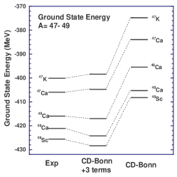
Figure 1: The experimental and theoretical ground state energy levels for $A=47-49$. The results in the second and third columns are labelled by their Hamiltonians.

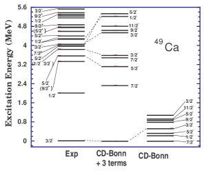
Figure 2: Experimental and theoretical excitation energy levels for ${}^{49}{Ca}$. Both CD-Bonn and CD-Bonn+3terms results are presented.

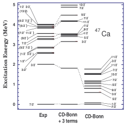
Figure 3: Experimental and theoretical excitation energy levels for ${}^{47}{Ca}$. Both CD-Bonn and CD-Bonn+3terms results are presented.

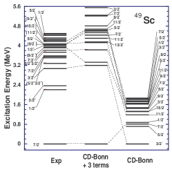
Figure 4: Experimental and theoretical excitation energy levels for ${}^{49}{Sc}$. Both CD-Bonn and CD-Bonn+3terms results are presented.

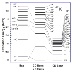
Figure 5: Experimental and theoretical excitation energy levels for ${}^{47}{K}$. Both CD-Bonn and CD-Bonn+3terms results are presented.

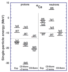
Figure 6: Experimental and theoretical levels that are dominantly single-proton and single-neutron particles or holes of ${}^{48}{Ca}$. The levels are labeled by (n, l, 2j), and the dashed lines are the Fermi energies.

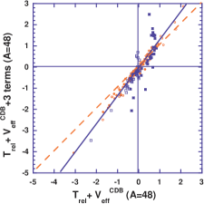
Figure 7: (color online) Correlation of $V(abcd;JT)$ matrix elements between CD-Bonn+3terms and CD-Bonn. The matrix elements of $T=0$ and $T=1$ are shown by circles and squares, respectively. The filled circles and the filled squares are for all $V(abab;JT)$ matrix elements that contribute to the monopole $V(ab;T)$. The open circles and open squares are for all the remaining matrix elements. There are no monopole shifts. The solid straight line represents a linear fit to all the matrix elements. The diagonal dashed line represents the reference correlation line at $45$-degrees.

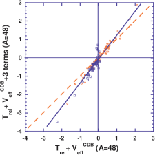
Figure 8: (color online) Correlation of $V(abcd;JT)$ between CD-Bonn+3terms and CD-Bonn, where we removed all $V(abab;JT)$ matrix elements that contribute to the monopole $V(ab;T)$. The solid straight line represents a linear fit to all the plotted points. The open circles and the open squares stand for $T=0$ and $T=1$, respectively. The diagonal dashed line represents the reference correlation line at $45$-degrees.

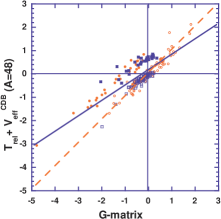
Figure 9: (color online) Correlation of $V(abcd;JT)$ matrix elements between CD-Bonn and G-matrix. See the caption to Fig. 8.

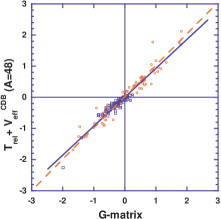
Figure 10: (color online) Correlation of $V(abcd;JT)$ between CD-Bonn and G. See the caption to Fig. 8.

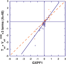
Figure 11: (color online) Correlation of the matrix elements $V(abcd;JT)$ between CD-Bonn+3terms and GXPF1, where we retain only the off-diagonal matrix elements, i.e. the $56$ matrix elements that cannot contribute to a single-particle Hamiltonian (see text). The open circles and the open squares stand for $T=0$ and $T=1$, respectively. The thick solid line represents a linear fit to all the plotted points. The diagonal dashed line represents the reference correlation line at $45$-degrees.

III.2 Excitation energy spectra

The excitation energy spectra for ⁴⁹Ca, ⁴⁷Ca, ${}^{49}Sc$ and ⁴⁷K are shown in Figs. 2-6 respectively. In every case the ab initio NCSM results with CD-Bonn are far too compressed relative to experiment - a feature also seen in the $A=48$ results [VPSN06] . Here, we trace this primary defect to the inferred properties of the neutron orbits. That is, the incorrect ground state spin seen in Fig. 2 and the absence of a significant excitation energy gap in Fig. 4 indicate the spin-orbit splitting of the neutrons is insufficient to provide proper subshell closure at the neutron $0f_{7/2}$ orbit. This defect is rectified in the results with CD-Bonn + 3 terms as seen by the corresponding spectra in Figs. 2 and 4. Similar tendencies have been seen before with valence G-matrix interactions and identified as a problem with the $L^{2}$ dependence of the single-particle states [MZPC96] ; [Caurier05] .

The CD-Bonn results in Figs. 4 and 6 are more difficult to interpret due to the glaring deficiencies just mentioned for the neutrons with the CD-Bonn Hamiltonian. We will show below that the proton shell closure is better established with CD-Bonn. This supports the assertion that the main deficiencies seen in the third columns of Figs. 4 and 6 are indeed likely to reside with the inferred neutron spin-orbit splitting problem.

The modified Hamiltonian provides greatly improved spectra for all four nuclei as seen in the second columns of Figs. 2-6. It is to be noted that these nuclei were not involved in the fitting procedure used to determine the parameters of the added phenomenological terms. Perhaps the most significant remaining deficiency is the incorrect ground state spin for ⁴⁷K as seen in Fig. 6. This is the first case of a nucleus in the region of $A=47$ to $A=49$ (12 nuclei studied to date) where we did not obtain the correct ground state spin with CD-Bonn + 3 terms Hamiltonian.

III.3 Single-particle characteristics

In order to better understand the underlying physics of our NCSM results, we investigate the single-particle-like properties of our solutions.

In a simple closed-shell nucleus, we expect the leading configuration of the ground state solution in our m-scheme treatment to be a single Slater determinant. Single-particle (or hole) excitations should be easily identified by the character of their leading configurations - i.e. a single-particle creation (or destruction) operator acting on the ground state Slater determinant of the reference nucleus ⁴⁸Ca. For our odd-mass nuclei, this is the character we seek. That is, we take the standard phenomenological shell model configuration of a single Slater determinant with a closed $sd$-shell for the protons and a closed $f_{7/2}$ subshell for the neutrons and look for the appropriate states which have a single nucleon added to (or subtracted from) that Slater determinant. We accept states as “single-particle-like” when we find one with a leading configuration having more than 50% probability to be in the simple configuration just described. When the majority weight is distributed over a few states, we use the centroid and we discuss those cases in some detail below. We were not successful in locating all the expected single-particle-like and single-hole-like states. That is, those absent from our presentation below were spread among a large number of eigenstates.

For a closed-shell nucleus $(Z,N)$ the single-particle energies (SPE) for states above the Fermi surface are related to the binding energy differences:

$e_{p}^{>}=BE(Z,N)-BE^{*}(Z+1,N)$
and

$e_{n}^{>}=BE(Z,N)-BE^{*}(Z,N+1)$.

The SPE for sates below the Fermi surface are given by

$e_{p}^{<}=BE^{*}(Z-1,N)-BE(Z,N)$
and

$e_{n}^{<}=BE^{*}(Z,N-1)-BE(Z,N)$.

The BE are ground state binding energies which are taken as positive values, and $e$ will be negative for bound states. $(BE^{*}=BE-E_{x})$ is the ground state binding energy minus the excitation energy of the excited states associated with the single-particle states.

Experimental SPE’s and the results of our analysis are shown in Fig. 6. The experimental SPE’s for protons and neutrons follow B.A.Brown’s analysis [BAB01] . To guide the eye, we draw a horizontal line to indicate the vicinity of the Fermi surfaces for the protons and neutrons.

Fig. 6 shows that proton shell closure is established with both Hamiltonians, the CD-Bonn and the CD-Bonn+3 terms. The correct energy locations are better approximated with the modified Hamiltonian. Fig. 6 also shows that neutron subshell closure only appears with the modified Hamiltonian. Here, the ordering is correct but the states are considerably more spread out compared with experiment.

Let us consider some of the details underlying the single-particle-like states. The situation for the $1p_{3/2}$ or “$1p3$” state in the left panel of Fig. 6, the proton single-particle state in ${}^{49}Sc$ with the modified Hamiltonian, is quite interesting. It appears that this state is mixed over several excited states in the spectrum. We can take the strength spread over several states and construct a centroid for this $1p3$ state by a weighted average over the states carrying that strength. Here are the relevant input ingredients.

The first excited state of ${}^{49}Sc$ is a ${3/2}^{-}$, as seen in the second column of Fig. 4, with about 51% of the occupancy of the $1p3$ state. Its eigenvalue is $-425.151$ MeV compared to a ground state of $-428.365$ MeV. The $18th$ state in the ${}^{49}Sc$ spectrum is also a ${3/2}^{-}$ with 28% of the occupancy of the $1p3$ state. Its eigenvalue is $-422.803$ MeV. The $24th$ state is also a ${3/2}^{-}$ with 21% of the occupancy of the $1p3$ state. Its eigenvalue is $-422.440$ MeV.

Thus, to a good approximation, the $1p3$ strength is spread over these three states. We will identify the weighted average $[0.51\times(-425.151)+0.28\times(-422.803)+0.21\times(-422.440)]=-423.79$ as the centroid of the single particle $1p3$ state which we then include accordingly in the second column of the figure.

For the proton hole states with the modified Hamiltonian, we perform a detailed search up to excitation energies of about $14$ MeV in the ⁴⁷K spectra. It appears that the $0d_{5/2}$ single-hole state is spread among many states with the largest observed concentration on the ${5/2}^{+}$ state at $-386.17$ MeV (13.36 MeV of excitation energy). Here, we find a single $J^{\pi}={5/2}^{+}$ state in ⁴⁷K with 30 % $0d_{5/2}$ vacancy and we assign this state to our $0d_{5/2}$ single-hole state. Most of the $0d_{5/2}$ strength, however, was not observed among the limited number of converged eigenstates.

Let us consider the ⁴⁹Ca results with the modified Hamiltonian in the upper right panel of Fig. 6. The ground state is approximately a pure $[(1p_{3/2})^{1}(0f_{7/2})^{8}]$ configuration. We note that the spacing for the subshell closure is in good agreement with experiment while there is a shift of a couple MeV towards more binding in the model as previously indicated in Fig. 2. A nearly pure $1p_{1/2}$ single-particle state is obtained at 5.235 MeV excitation energy and an extra low-lying ${7/2}^{-}$ appears with $2p-1h$ character (see Fig. 2). Our lowest-lying ${5/2}^{-}$ consists of $2p-1h$ character relative to subshell closure.

We contrast the modified Hamiltonian’s results for the ⁴⁹Ca ground state with those obtained using the ab initio CD-Bonn where $[(1p_{3/2})^{4}(1p_{1/2})^{2}(0f_{7/2})^{3}]_{1/2^{-}}$ is the dominant configuration reflecting again the inadequacies of the neutron single-particle properties with CD-Bonn.

III.4 Monopole matrix elements V(ab;T)

The monopole matrix element is defined by an angular momentum average of coupled doubly-reduced two-body matrix elements:

$$V(ab;T)=\frac{\sum_{J}(2J+1)V(abab;JT)}{\sum_{J}(2J+1)}\;.$$ (3)

For our NCSM Hamiltonians the “$V$” appearing in Eqn.

3 signifies the full 2-body intrinsic-coordinate Hamiltonian, $T_{rel}+V_{eff}$, except that we omit the Coulomb interaction from this analysis.

We examined the monopole character of our initial CD-Bonn Hamiltonian and we compared it with the monopole features of the GXPF1 interaction[HOB04] . Although the monopole characteristics were similar, we do not present the detailed comparisons here due to the ambiguity of the role of the SPE’s. That is, one may shift some Hamiltonian components between SPE’s and two-body matrix elements (TBME’s) and this obscures direct comparisons of a subset of our TBME’s with the corresponding subset of GXPF1. In order to summarize a comparison of the underlying theoretical interactions, we list in Table 1 a simplified overview of their differences and similarities.

For a sample comparison of the interactions, we present a small set of two-body $fp$-shell matrix elements applicable to the present investigation in Table 2. For convenience we present two columns of key differences in the matrix elements: “diff1” represents the difference between the G-matrix and the GXPF1 interaction resulting from adjusting the G-matrix elements to fit spectra; and, “diff2” represents the difference between our ab initio $H_{eff}$ and our modified $H_{eff}$. The scale of the changes from the respective starting solutions appears comparable, though one of the ”diff2” values reaches -1.2123 MeV.

III.5 Matrix element correlations

We present in Figs. 8 - 11 the correlations between pairs of $fp$-shell interaction matrix element sets. With Fig. 8, we observe the high degree of correlation between the 195 matrix elements of our starting Hamiltonian, CD-Bonn, and our modified Hamiltonian, CD-Bonn + 3 terms. This indicates that, for the most part, our Hamiltonian is minimally modified by the addition of the phenomenological terms. Such a high correlation is reminiscent of the high correlations seen between GXPF1 and its starting interaction, the G-matrix [HOB04] . It is interesting to see if certain groups of matrix elements appear to be more correlated than the others. We distinguish the diagonal $V(abab;JT)$ matrix elements that contribute to the monopole by different symbols. Filled circles stand for $V(abab;JT=0)$ and filled squares stand for $V(abab;JT=1)$ matrix elements. All the remaining matrix elements $V(abcd;JT)$ where at least one single-particle-state (sps) of the bra is different from a sps of the ket are plotted as open circles for $T=0$ and open squares for $T=1$. We see the filled square points, that correspond to $V(abab;JT=1)$ matrix elements, are farther from the linear fit, ranging between 1 MeV and 2 MeV away from the linear fit line. Therefore, these monopole matrix elements have received larger corrections than others in the process of fitting the $A=48$ isotopes.

In the forth paragraph of the same subsection we changed the sentence ”The colors and the symbols used are the same as those in figures 7 and 8.” with ”The symbols used are the same as those in figures 7 and 8.”

To see the stronger correlations more clearly, we next choose in Fig. 8 to eliminate all matrix elements contributing to the monopole. There are 135 remaining matrix elements out of the 195 total. The degree of correlation between the 135 matrix elements significantly improves with much less deviation from the linear fit. We can see another feature of the correlation by comparing the linear fit with the $45$-degree line in Fig. 8 (similar pattern seen in Fig. 8). On the one hand, we see that the CD-Bonn + 3 terms matrix elements are shifted towards greater attraction where CD-Bonn is already attractive. On the other hand, the CD-Bonn + 3 terms matrix elements are shifted towards greater repulsion where CD-Bonn is already repulsive. Overall, we observe that the larger differences between the CD-Bonn and CD-Bonn + 3 terms are coming from the monopole terms. This seems natural in light of the fact that the phenomenological terms have the effect of adjusting the single particle features of the theory towards agreement with experiment. That is, the monopole terms receive the largest adjustments as required to achieve the needed single particle features.

It is then very interesting to observe in Fig. 10 the lack of correlation between our starting Hamiltonian, CD-Bonn, and the G-matrix underlying the GXPF1 interaction. Points are generally farther away from the fit line than in the correlation of CD-Bonn + 3 terms with CD-Bonn case. Note that the G-matrix is a renormalization procedure and the specific results for GXPF1 are developed from the bare CD-Bonn interaction. This lack of correlation in Fig. 10 reflects the major differences in the underlying effective interaction theories that are summarized in Table 1.

We now make the same set of comparisons between CD-Bonn and G-matrix in Figs. 10 and 10 as we performed in Figs. 8 and 8. The symbols used are the same as those in Figs. 8 and 8. Comparing Fig. 10 and Fig. 10 we can see how, after eliminating the matrix elements that contribute to the monopole, the correlation is significantly improved with the linear fit in Fig. 10 and it now overlaps well with the 45-degree line. Again, this shows similarities between these two interactions with the difference arising primarily from the monopole part.

We can comment further about the comparison presented in Fig. 10 by observing that the full Hamiltonian developed from the G-matrix includes single-particle energy (SPE) contributions. On the other hand CD-Bonn does not have additional SPE contributions since those contributions are already included in the 2-body matrix elements. In fact, those SPE contributions to our interactions are embedded in the monopole terms. This is one reason why the correlations improve when we proceed from Fig. 10 to Fig. 10, removing the monopole terms.

Finally, in order to focus as clearly as possible on the 2-body interaction effects , we present in Fig. 11 the correlation of matrix elements $V(abcd;JT)$$(A=48)$ between CD-Bonn+3terms and GXPF1, where we retain only those that cannot contribute to a single-particle Hamiltonian. That is, we eliminate all two-body matrix elements where at least one single-particle-state (sps) of the bra equals a sps of the ket. There are 56 remaining two-body matrix elements. Differences ranging up to about 3 MeV are observed which should lead to differences in experimental observables. Comparisons of spectra and other properties with these Hamiltonians, as one proceeds further from $A=48$, could shed more light on their differences.

IV Conclusions and outlook

We have presented an initial NCSM investigation of the spectral properties of the $A=47$ and $A=49$ nuclei that are one nucleon away from doubly-magic ⁴⁸Ca. We have shown that the NCSM with a previously introduced modified Hamiltonian produces spectral properties in reasonable accord with experiment. Shell closure and single-particle spectral properties are obtained indicating a path has been opened for multi-shell investigations of these nuclei within the NCSM. We are undertaking such additional investigations. Also, for a better understanding of various $fp$-shell interactions we made a comparison between our initial and modified $fp$-shell matrix elements in the harmonic oscillator basis with the GXPF1 interaction [HOB04] . Our initial and modified NCSM $H_{eff}$ matrix elements in the $fp$-shell are strongly correlated. We found some evidence suggesting that significant differences in single-particle properties may underly some of the distinctions between our $H_{eff}$ and the GXPF1 interaction. The differences were reduced when we compared the purely off-diagonal matrix elements in Fig. 11. Additional applications could reveal the importance of these distinctions in greater detail.

V Acknowledgements

This work was partly performed under the auspices of the U. S. Department of Energy by the University of California, Lawrence Livermore National Laboratory under contract No. W-7405-Eng-48. This work was also supported in part by USDOE grants DE-FG02-87ER40371 and DE-FC02-09ER41582, Division of Nuclear Physics, and, in part, by NSF grant INT0070789.

Hamiltonian Property	G-matrix	NCSM cluster $H_{eff}$
Oscillator parameter dependence	Yes	Yes
Depends on the choice of P-space	Yes	Yes
Reguires effective multi-nucleon
interactions as corrections	Yes	Yes
Translationally invariant	No	Yes
Starting energy dependence	Yes	No
Single-particle spectra dependence	Yes	No
$A$-dependence	No	Yes

Table 1: Overview of the differences and similarities of the two theoretical approaches that underlie the Hamiltonians whose matrix elements are compared in this work.

$2j_{a}$	$2j_{b}$	$2j_{c}$	$2j_{d}$	J	T	G	GXPF1	diff1	CD-Bonn	CD-Bonn	diff2
										+3 terms
7	3	7	3	5	0	-2.1167	-2.8504	-0.7337	-1.0390	-1.3413	-0.3023
3	3	5	5	0	1	-0.5243	-1.1968	-0.6725	-0.6019	-1.1129	-0.5109
7	7	7	7	3	0	-0.2309	-0.8087	-0.5778	0.5597	0.5555	-0.0042
7	5	7	5	6	0	-2.3465	-2.9159	-0.5693	-1.3743	-1.8599	-0.4856
7	5	7	5	5	0	-0.0203	-0.5845	-0.5642	0.5813	0.4117	-0.1693
3	1	3	1	2	1	-0.7965	-0.2822	0.5143	-0.0068	-0.4932	-0.4864
7	7	5	5	0	1	-1.9095	-1.3288	0.5806	-2.2586	-3.4709	-1.2123

Table 2: Comparison of selected two-body matrix elements $V(abcd;JT)$ (Mev) $(A=48)$ for which the difference between our interaction is large. “diff1” represents the difference between GXPF1 and G while “diff2” is the difference between CD-Bonn+3terms and CD-Bonn.

References

- (1) T. W. Burrows, Nucl. Data Sheets, 74, 1 (1995); Nucl. Data Sheets 76, 191 (1995).
- (2) Electronic version of Nucl. Data Sheets, telnet://bnlnd2..dne.bnl.gov
- (3) G. Martinez-Pinedo, A. P. Zuker, A. Poves and E. Caurier, Phys. Rev. C 55 187 (1997); nucl-th/9608044.
- (4) B. A. Brown, Progr. Part. Nucl. Phys. 47, 517 (2001).
- (5) T. Otsuka, M. Honma, T. Mizusaki, N. Shimizu, and Y. Utsuno, Prog. Part. Nucl. Phys. 47, 319 (2001).
- (6) D. J. Dean, T. Engeland, M. Hjorth-Jensen, M. Kartamychev and E. Osnes, Prog. Part. Nucl. Phys. 53 419(2004).
- (7) E. Caurier, G. Martinez-Pinedo, F. Nowacki, A. Poves and A. P. Zuker, Rev. Mod. Phys. 77 427(2005).
- (8) A. Poves, E. Pasquini and A. P. Zuker, Phys. Lett. B82, 319 (1979); A. Poves and A.P. Zuker, Phys. Rep. 70, 235 (1981).
- (9) J. P. Vary, S. Popescu, S. Stoica and P. Navrátil, J. Phys. G: Nucl. Part. Phys. 36 085103(2009), nucl-th 0607041.
- (10) J. P. Vary, “Many-Fermion Dynamics Code,” (1992, unpublished); J. P. Vary and D. C. Zheng, ibid, (1994,unpublished).
- (11) R. Machleidt, F. Sammarruca and Y. Song, Phys. Rev. C 53, 1483 (1996); R. Machleidt, Phys. Rev. C 63, 024001 (2001).
- (12) M. Honma, T. Otsuka, B. A. Brown and T. Mizusaki, Phys. Rev. C 65, 061301(r) (2002); Phys. Rev. C 69, 034335 (2004).
- (13) K. D. Sviratcheva, J. P. Draayer and J. P. Vary, Proceedings of the XXV International Workshop on Nuclear Theory (June 26 - July 1, 2006, Rila), ed. S. Dimitrova (DioMira, Sofia, Bulgaria, 2006) 225-234; nucl-th/0703067.
- (14) K. D. Sviratcheva, J. P. Draayer and J.Vary, Phys. Rev. C 73, 034324 (2006);nucl-th/0703075; Nuclear Physics A 786, 31(2007); nucl-th/0703076.
- (15) A. F. Lisetskiy, B. R. Barrett, M. K. G. Kruse, P. Navratil, I. Stetcu, J. P. Vary, Phys. Rev. C. 78, 044302 (2008).
- (16) A. F. Lisetskiy, M. K. G. Kruse, B. R. Barrett, P. Navratil, I. Stetcu and J.P. Vary, Phys. Rev. C 80, 024315(2009).
- (17) M. Hjorth-Jensen, T. T. S. Kuo and E. Osnes, Phys. Repts. 261, 125 (1995).
- (18) D. C. Zheng, B. R. Barrett, L. Jaqua, J. P. Vary, and R. L. McCarthy, Phys. Rev. C 48, 1083 (1993); D. C. Zheng, J. P. Vary, and B. R. Barrett, Phys. Rev. C 50, 2841 (1994); D. C. Zheng, B. R. Barrett, J. P. Vary, W. C. Haxton, and C. L. Song, Phys. Rev. C 52, 2488 (1995).
- (19) P. Navrátil and B. R. Barrett, Phys. Rev. C 54, 2986 (1996); Phys. Rev. C 57, 3119 (1998).
- (20) P. Navrátil and B. R. Barrett, Phys. Rev. C 57, 562 (1998).
- (21) P. Navrátil and B. R. Barrett, Phys. Rev. C 59, 1906 (1999); P. Navrátil, G. P. Kamuntavičius and B. R. Barrett, Phys. Rev. C 61, 044001 (2000).
- (22) P. Navrátil, J. P. Vary and B. R. Barrett, Phys. Rev. Lett. 84, 5728 (2000); Phys. Rev. C 62, 054311 (2000).
- (23) P. Navrátil, J. P. Vary, W. E. Ormand and B. R. Barrett, Phys. Rev. Lett. 87, 172502 (2001); E. Caurier, P. Navrátil, W. E. Ormand and J. P. Vary, Phys. Rev. C 64, 051301 (2001).
- (24) S. Okubo, Prog. Theor. Phys. 12, 603 (1954); J. Da Providencia and C. M. Shakin, Ann. of Phys. 30, 95 (1964); S. Y. Lee and K. Suzuki, Phys. Lett. B 91, 173 (1980); K. Suzuki and S. Y. Lee, Prog. of Theor. Phys. 64, 2091 (1980); K. Suzuki, Prog. Theor. Phys. 68, 246 (1982); K. Suzuki, Prog. Theor. Phys. 68, 1999 (1982); K. Suzuki and R. Okamoto, Prog. Theor. Phys. 70, 439 (1983).
- (25) R. B. Wiringa, V. G. J. Stoks, and R. Schiavilla, Phys. Rev. C 51, 38 (1995).
- (26) C. P. Viazminsky and J. P. Vary, J. Math. Phys., 42, 2055 (2001).
- (27) H. Kamada, et. al, Phys. Rev. C 64 044001(2001).
- (28) I. Stetcu, B.R. Barrett, P. Navrátil and J. P. Vary, Phys. Rev. C 71, 044325(2005); I. Stetcu, B. R. Barrett, P. Navrátil and C. W. Johnson, Int. J. Mod. Phys. E 14, 95 (2005); I. Stetcu, B. R. Barrett, P. Navrátil and J. P. Vary, Phys. Rev. C 73, 037307(2006).
- (29) A. Nogga, P. Navrátil, B.R. Barrett and J. P. Vary, Phys. Rev. C 73, 064002 (2006), and references therein.
- (30) M. A. Hasan, J. P. Vary, and P. Navrátil, Phys. Rev. C 69, 034332 (2004) .
- (31) A. C. Hayes, P. Navrátil and J. P. Vary, Phys. Rev. Lett. 91, 012502 (2003).
- (32) A. M. Shirokov, A. I. Mazur, S. A. Zaytsev, J. P. Vary and T. A. Weber, Phys. Rev. C 70, 044005 (2004).
- (33) A. M. Shirokov, J. P. Vary, A. I. Mazur, S. A. Zaytsev and T. A. Weber, Phys. Letts. B 621, 96 (2005).
- (34) A. M. Shirokov, J. P. Vary, A. I. Mazur and T. A. Weber, Phys. Letts. B 644, 33(2007), nucl-th/0512105.
- (35) P. Navrátil, V. G. Gueorguiev, J. P. Vary, W. E. Ormand and A. Nogga, Phys. Rev. Lett. 99, 042501(2007); nucl-th 0701038.
- (36) C. Forssen, J. P. Vary, E. Caurier and P. Navratil, Phys. Rev. C 77, 024301 (2008); arXiv 0802.1611.
- (37) S. K. Bogner, R. J. Furnstahl, P. Maris, R. J. Perry, A. Schwenk and J. P. Vary, Nucl. Phys. A 801, 21(2008); arXiv:0708.3754.
- (38) P. Maris, J.P. Vary and A. M. Shirokov, Phys. Rev. C. 79, 014308(2009), DOI: 10.1103/PhysRevC.79.014308, arXiv 0808.3420.
- (39) R. J. Lloyd and J. P. Vary, Phys. Rev. D 70: 014009 (2004), hep-ph/0311179; J. P. Vary, D. Chakrabarti, A. Harindranath, R. J. Lloyd, L. Martinovic and J. R. Spence, Nucl. Phys. B 161, 223 (2006); J. P. Vary, H. Honkanen, J. Li, P. Maris, S. J. Brodsky, P. Sternberg, E. G. Ng and C. Yang, Recent Progress in Hamiltonian light-front QCD, in Light Cone 2008 Relativistic Nuclear and Particle Physics, Proceedings of Science LC2008 (Sissa, IT), 040 (2008), 040 (2008) ; SLAC-PUB-13460; arXiv: 0812.1819.