Topological confinement in graphene bilayer quantum rings

Abstract

We demonstrate the existence of localized electron and hole states in a ring-shaped potential kink in biased bilayer graphene. Within the continuum description, we show that for sharp potential steps the Dirac equation describing carrier states close to the $K$ (or $K^{\prime}$) point of the first Brillouin zone can be solved analytically for a circular kink/anti-kink dot. The solutions exhibit interfacial states which exhibit Aharonov-Bohm oscillations as functions of the height of the potential step and/or the radius of the ring.

Graphene, a one atom thick crystal sheet of carbon, has been shown to display striking electronic and mechanical properties which are expected to lead to the development of new devices (for a review, see e.g. Castro1 ). These properties are related to the unusual electronic structure of graphene, in which the charge carriers behave as massless fermions with a gapless linear dispersion. For two coupled graphene sheets, known as bilayer graphene (BG), the electronic structure is modified due to the interlayer interaction, with the otherwise linear dispersion becoming approximately parabolic. Another important feature of BG is the fact that the electronic dispersion can develop a gap, either by doping of one of the layers or by the application of an external perpendicular electric field. Such a gap can be tuned by varying the external electric field Falko , which allows for the possibility of tailoring the electronic structure of BG for the development of devices, such as quantum dots Milton1 ; Magdot , and quantum rings Zarenia1 ; Zarenia2 . Recently it has been shown that another consequence of the existence of a tunable gap in BG is the possibility of topological confinement of carriers in antisymmetric potential ’kinks’, i.e. at the interface between two regions of an antisymmetric external electric field Morpurgo ; Martinez ; SanJose . These states have similarities with the surface states of topological insulators topoinsul1 ; topoinsul2 . Their energies are found inside the gap and the wavefunctions are predicted to decay away from the interface of the kink potential. These topological states are expected to be robust with respect to the effect of disorder, with the carrier propagation along the potential kink displaying electron-hole asymmetry. In addition, the geometry of the potential interface is determined by the shape of the voltage gates used to induce the gap. That in turn can be used to further constrain the carrier propagation.

In this letter we propose a system in which topological confined states are realized at the interface of a kink potential shaped as a ring. This system can be regarded as a good approximation of an ideal quantum ring of zero width. We obtain analytical expressions for the electronic wavefunction of the BG four-band Hamiltonian. Bilayer graphene can be described as two bipartite coupled sheets with four triangular sublattices labeled as $A$ ($A^{\prime}$) and $B$ ($B^{\prime}$) in the upper (lower) layer. For Bernal stacking Milton2 the coupling between layers is described by the hopping energy $\overline{t}$ = 400 meV between sites $A$ and $B^{\prime}$, so that the Hamiltonian around the $K$ point of the first Brillouin zone can be written as

$$H=\left[\begin{array}[]{cccc}\overline{U}_{1}&\pi&\overline{t}&0\\ \pi^{\dagger}&\overline{U}_{1}&0&0\\ \overline{t}&0&\overline{U}_{2}&\pi^{\dagger}\\ 0&0&\pi&\overline{U}_{2}\end{array}\right],$$ (1)

where $\overline{U}_{1}$ and $\overline{U}_{2}$ are external electrostatic potentials applied respectively to the upper and lower layers. In polar coordinates we have $\pi=-i\hbar v_{F}e^{i\theta}\left(\frac{\partial}{\partial{\rho}}+\frac{i}{\rho}\frac{\partial}{\partial{\theta}}\right)$ and $\pi^{\dagger}=-i\hbar v_{F}e^{-i\theta}\left(\frac{\partial}{\partial{\rho}}-\frac{i}{\rho}\frac{\partial}{\partial{\theta}}\right)$. The eigenstates of the Hamiltonian Eq. (1) are four component pseudo-spinors $\Psi=\left[\psi_{A},\quad\psi_{B},\quad\psi_{B^{\prime}},\quad\psi_{A^{\prime}}\right]^{T}$, where $\psi_{A}$ and $\psi_{B}$ ($\psi_{A^{\prime}}$ and $\psi_{B^{\prime}}$) are the envelope functions for the probability amplitudes for sublattices $A$ ($A^{\prime}$) and $B$ ($B^{\prime}$), respectively, in the upper (lower) layer. The resulting four coupled differential equations can be decoupled, giving, for $\overline{U}_{2}=-\overline{U}_{1}$

$$\nabla^{2}\nabla^{2}\psi_{A}+2(\epsilon^{2}+U_{1}^{2})\nabla^{2}\psi_{A}+$$ (2)

(3)

$$+[(U_{1}^{2}-\epsilon^{2})^{2}+t^{2}(U_{1}^{2}-\epsilon^{2})]\psi_{A}=0,$$ (4)

with $U_{1}=\overline{U}_{1}/\hbar v_{F}$, $U_{2}=\overline{U}_{2}/\hbar v_{F}$, $t=\overline{t}/\hbar v_{F}$ and $\epsilon=E/\hbar v_{F}$, where $E$ is the energy.

For the case of a quantum ring with radius $R$, following Ref. Morpurgo , we assume a sharp potential kink, so that one can define two regions, namely I) $0\leq\rho<R$ and II) $\rho>R$. The upper inset of Fig. 1 illustrates a sketch of the system considered in the present letter. In order to simplify the calculations, the potentials $U_{1}$ (red, dashed-dotted) and $U_{2}$ (blue, solid) are assumed to be piecewise constant, defined as $V$ and $-V$ for region I and $-V$ and $V$ for region II, respectively, as illustrated in the lower inset of Fig. 1. Notice that this quantum ring potential is different from the one studied in Ref. Zarenia1 , where the potential was defined as zero inside a finite width circular ring and $U_{1}=-U_{2}=V$ otherwise. In order to obtain an analytical solution for this problem, one must solve the system of differential equations for each region and match the eigenfunction at the boundaries. For region I the solutions are Bessel functions, which obey the relation $\nabla^{2}F_{m}(\alpha\rho)e^{im\theta}=\pm\alpha^{2}F_{m}(\alpha\rho)e^{im\theta}$, where the function $F_{m}(\alpha\rho)$ denotes the Bessel functions $J_{m}(\alpha\rho)$ or $Y_{m}(\alpha\rho)$, with eigenvalue $+\alpha^{2}$, or the modified Bessel functions $I_{m}(\alpha\rho)$ or $K_{m}(\alpha\rho)$, with eigenvalue $-\alpha^{2}$. The circular symmetry of the problem implies that $m=0,\pm 1,\pm 2,...$. By substituting the solutions one finds a fourth order algebraic equation for $\alpha$, whose solutions are

$$\alpha=\pm\sqrt{V^{2}+E^{2}\pm\sqrt{4V^{2}E^{2}-t^{2}(V^{2}-E^{2})}}$$ (5)

Henceforth, we consider only energies within the interval where $\alpha$ is complex, such that $F_{m}(\alpha\rho)$ exhibits real and imaginary parts. If one chooses $\alpha=\sqrt{V^{2}+E^{2}-\sqrt{4V^{2}E^{2}-t^{2}(V^{2}-E^{2})}}$, four linearly independent (LI) solutions are found: $\Re[J_{m}(\alpha\rho)]e^{im\theta}$, $\Im[J_{m}(\alpha\rho)]e^{im\theta}$, $\Re[K_{m}(i\alpha\rho)]e^{im\theta}$ and $\Im[K_{m}(i\alpha\rho)]e^{im\theta}$. It can be verified that these functions are solutions of Eq. (4), although they are not separately eigenfunctions of the Laplacian. It is important to point out that, for this choice of $\alpha$, this set of functions is LI only when the imaginary part of $\alpha$ is negative.

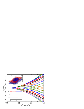
Figure 1: (Color online) Energy states with angular momentum index $m=0,\pm 1,...,\pm 5$ as a function of the square root of the kink/anti-kink potential height (lower inset) for a bilayer graphene ring as schematically shown in the upper inset, considering a ring radius $R=50$ nm. Full (empty) symbols refer to negative (positive) $m$. The black solid lines depicts the limits $\pm V$ between the confined states and the continuum, whereas the thin dotted line is $E=0$.

The functions $\Re[J_{m}(\alpha\rho)]e^{im\theta}$ and $\Im[J_{m}(\alpha\rho)]e^{im\theta}$ are finite at the origin, but diverge as $\rho\rightarrow\infty$ for any value of $m$. On the other hand, $\Re[K_{m}(i\alpha\rho)]e^{im\theta}$ diverges for $\rho\rightarrow 0$ and vanishes when $\rho\rightarrow\infty$, for any value of $m$. The function $\Im[K_{m}(i\alpha\rho)]e^{im\theta}$ has the same behavior as $\Re[K_{m}(i\alpha\rho)]e^{im\theta}$ for $m\neq 0$, but for $m=0$ it is finite at the origin. Based on this we construct the wavefunction $\phi_{A}^{<}$ for the region I as foot1

$$\psi_{A}^{<}(\rho,\theta)=\{A\Re[J_{m}(\alpha\rho)]+B\Im[J_{m}(\alpha\rho)]\}e^{im\theta}.$$ (6)

Using this expression for $\psi_{A}^{<}$, the radial part of the other components of $\Psi^{<}$ for region I are

$$\phi_{B}^{<}(\rho)=\frac{i}{V-E}\{A\Re[\alpha J_{m-1}(\alpha\rho)]+B\Im[\alpha J_{m-1}(\alpha\rho)]\},$$ (7)

$$\phi_{B^{\prime}}^{<}(\rho)=\frac{1}{t(V-E)}\{A\Re[\gamma_{1}J_{m}(\alpha\rho)]+B\Im[\gamma_{1}J_{m}(\alpha\rho)]\},$$ (8)

$$\phi_{A^{\prime}}^{<}(\rho) = \frac{i}{t(V^{2}-E^{2})}\{A\Re[\alpha\gamma_{1}J_{m+1}(\alpha\rho)]+$$ (11)

$$B\Im[\alpha\gamma_{1}J_{m+1}(\alpha\rho)]\},$$

where $\gamma_{1}=\alpha^{2}-(V-E)^{2}$ and $\psi_{B}^{<}(\rho,\theta)=\phi_{B}^{<}(\rho)e^{i(m-1)\theta}$, $\psi_{B^{\prime}}^{<}(\rho,\theta)=\phi_{B^{\prime}}^{<}(\rho)e^{i(m)\theta}$, and $\psi_{A^{\prime}}^{<}(\rho,\theta)=\phi_{A^{\prime}}^{<}(\rho)e^{i(m+1)\theta}$. Similarly, for region II, we choose for the wavefunction $\psi_{A}^{>}$ a linear combination of solutions that go to zero as $r\rightarrow\infty$, namely,

$$\psi_{A}^{>}(\rho,\theta)=\{C\Re[K_{m}(i\alpha\rho)]+D\Im[K_{m}(i\alpha\rho)]\}e^{im\theta},$$ (12)

and find the other components of $\Psi^{>}$ as

$$\phi_{B}^{>}(\rho) = \frac{i}{(V+E)}\{-C\Im[\alpha K_{m-1}(i\alpha\rho)]+$$ (15)

$$D\Re[\alpha K_{m-1}(i\alpha\rho)]\},$$

$$\phi_{B^{\prime}}^{>}(\rho) = \frac{-1}{t(V+E)}\{C\Re[\gamma_{2}K_{m}(i\alpha\rho)]+$$ (18)

$$D\Im[\gamma_{2}K_{m}(i\alpha\rho)]\},$$

$$\phi_{A^{\prime}}^{>}(\rho) = \frac{i}{t(V^{2}-E^{2})}\{-C\Im[\alpha\gamma_{2}K_{m+1}(i\alpha\rho)]+$$ (21)

$$D\Re[\alpha\gamma_{2}K_{m+1}(i\alpha\rho)]\},$$

where $\gamma_{2}=\alpha^{2}-(V+E)^{2}$ and $\psi_{B}^{>}(\rho,\theta)=\phi_{B}^{>}(\rho)e^{i(m-1)\theta}$, $\psi_{B^{\prime}}^{>}(\rho,\theta)=\phi_{B^{\prime}}^{>}(\rho)e^{i(m)\theta}$ and $\psi_{A^{\prime}}^{>}(\rho,\theta)=\phi_{A^{\prime}}^{>}(\rho)e^{i(m+1)\theta}$. The continuity of the wavefunction at $\rho=R$ implies that $\Psi^{<}(R,\theta)=\Psi^{>}(R,\theta)$. That condition leads to a system of equations from which we obtain the energy eigenvalues.

The energies of the topologically confined states of a bilayer graphene ring with radius $R=50$ nm are shown in Fig. 1 as function of the square root of the kink/anti-kink potential height. The energy spectrum exhibits the symmetry $E(m)=-E(-m)$, which corresponds to $E(k_{y})=-E(-k_{y})$ as found for a one-dimensional kink/anti-kink potential in the $x$-direction Morpurgo . Notice that the $m=0$ state is not the lowest energy state, and the less energetic confined electrons in such a system will have non-zero angular momentum index, even in the absence of a magnetic field. The zero energy states are two-fold degenerate (without taking spins into account), and are realized only for specific values of the potential height $V$.

Figure 2: (Color online) Energy spectrum for $m=0,\pm 1,...,\pm 7$ as a function of the ring radius for bilayer graphene in the presence of a circular kink/anti-kink potential of height $V=20$ meV. Full (empty) symbols refer to negative (positive) values of $m$. Three lines are drawn to help visualization: the black solid lines delimits the potential height $\pm V$, whereas the thin dotted line is $E=0$.

Figure 2 shows the energy states with angular momentum index $m=0,\pm 1,...,\pm 7$ as a function of the ring radius $R$ for a kink/anti-kink potential height $V=20$ meV. The solid lines delimits the -20 meV $<E<$ 20 meV energy spectrum of confined states. Notice that double degenerate $E=0$ states are observed only for specific values of the radius. The energies converge to two values, $\pm E_{c}$, as the ring radius increases, forming two merged bands around these energies. The value $E_{c}\simeq 13.9$ meV is identical to the energy of the corresponding one-dimensional problem with $k_{y}=0$.

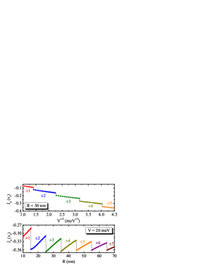
Figure 3: (Color online) Angular component of the probability density current as a function of the square root of the kink/anti-kink potential height $V$ (top), for a ring radius $R=50$ nm, and as a function of $R$ (bottom), when $V=20$ meV. The number on each curve refers to the angular momentum index $m$, and the solid curves are a guide to the eyes.

The origin of the zero energy states in Figs. 1 and 2 is similar to those found earlier for the one-dimensional problem: the energy spectrum for a kink/anti-kink potential, as shown in Ref. Morpurgo , exhibits $E=0$ states at two values of the linear momentum $\hbar k_{y}$ with the same modulus, say, $\hbar k_{y}^{(0)}$ and $-\hbar k_{y}^{(0)}$, which were shown to be proportional to the square root of the potential height $V$ for $V\ll t$. In the bilayer graphene ring problem, an analogy can be made between the angular momentum $L_{z}=\hbar m/R$ (see e. g. Eq. (23) of Ref. Zarenia2 ) and the linear momentum $\hbar k_{y}$ of the one-dimensional case. Whenever $L_{z}=\hbar m/R=\pm\hbar k_{y}^{(0)}$, zero energy states appear, hence, if one fixes the potential height $V$, $k_{y}^{(0)}$ will be a fixed value, and for each value of $m$, there will be a value of $R$ that satisfies this condition, leading to a double degenerate zero energy state for this value of the radius. For example, Fig. 2 shows the results for $V=20$ meV, where $k_{y}^{(0)}$ is found to be $\sim 0.1$ nm^-1, consequently, zero energy states are observed at $R\sim 10$ nm for $m=\pm 1$, $R\sim 20$ nm for $m=\pm 2$ and so on. Moreover, as the $E=0$ states satisfy the condition $m/R=k_{y}^{(0)}\simeq\sqrt{tV}/(2^{3/4})$ for $V\ll t$ Morpurgo , the equally spaced zero energy states observed in Fig. 1 occur for $m/\sqrt{V}=2^{-3/4}R\sqrt{t}$, which for the parameters of Fig. 1 becomes $\sqrt{V}\sim 0.9$ meV^1/2 for $m=\pm 1$, $\sqrt{V}\sim 1.8$ meV^1/2 for $m=\pm 2$ and so on. It is worth to point out that the condition $k_{y}^{(0)}=\sqrt{tV}/(2^{3/4})$ proposed by Martin et al. Morpurgo for the one dimensional problem was obtained from the reduced 2 $\times$ 2 Hamiltonian, which is valid only for $V\ll t$, hence the dependence of $k_{y}^{(0)}$ on $\sqrt{V}$ is no longer guaranteed for large values of the kink/anti-kink potential height.

The fact that the energy of the lowest energy states oscillates as function of $R$ and $V$, where angular momentum transitions take place, suggests the possibility of observing persistent currents in each valley $K$ or $K^{\prime}$ induced by the external potential, in analogy to Aharonov-Bohm rings, but in the absence of a magnetic field. The angular component of the probability density current Zarenia2 for the lowest energy state is shown as a function of the kink/anti-kink potential $V$ (top) and the ring radius $R$ (bottom) in Fig. 3, where current jumps are observed when angular momentum transitions occur between states with different $|m|$. We point out that $J_{\theta}(m)=J_{\theta}(-m)$ and that the current for $K$ and $K^{\prime}$ valleys have opposite sign, so that the net current, taking into account both valleys, is zero.

In summary, we demonstrated that confined quantum ring states can be realized in a circular kink/anti-kink potential in bilayer graphene. We obtained an analytical solution for the Dirac equation describing electrons close to the Dirac point. Zero energy states, with two-fold degeneracy, are realized for special values of the radius and potential height. Angular currents for the lowest energy state, which present oscillations due to angular momentum transitions as $V$ or $R$ increases, are observed. Although, for the sake of simplicity, the potential profile was assumed to be abrupt in the present work, in a more realistic description it should have a continuous shape. Nevertheless, the present results must give at least a good qualitative agreement with a kink/anti-kink BG ring, which would be helpful for the understanding of future experiments on such a system.

This work was financially supported by CNPq, under contract NanoBioEstruturas 555183/2005-0, FUNCAP, CAPES, the Bilateral programme between Flanders and Brazil, the Belgian Science Policy (IAP) and the Flemish Science Foundation (FWO-Vl).

References

- (1) A. H. Castro Neto, F. Guinea, N. M. R. Peres, K. S. Novoselov, and A. Geim, Rev. Mod. Phys. 81, 109 (2009).
- (2) E. McCann and V. I. Fal’ko, Phys. Rev. Lett. 96, 086805 (2006).
- (3) J. M. Pereira Jr., P. Vasilopoulos, and F. M. Peeters, Nano Lett. 7, 946, (2007).
- (4) J. M. Pereira Jr., F. M. Peeters, P. Vasilopoulos, R. N. Costa, and G. A. Farias, Phys. Rev. B 79, 195403 (2009). (2006).
- (5) M. Zarenia, J. M. Pereira Jr., F. M. Peeters, and G. A. Farias, Nano Lett. 9, 4088 (2009).
- (6) M. Zarenia, J. M. Pereira Jr., A. Chaves, F. M. Peeters, and G. A. Farias, Phys. Rev. B 81, 045431 (2010).
- (7) I. Martin, Ya. M. Blanter, and A. F. Morpurgo, Phys. Rev. Lett. 100, 036804 (2008).
- (8) J. C. Martinez, M. B. A. Jalil, and S. G. Tan, Appl. Phys. Lett. 95, 213106 (2009).
- (9) P. San-Jose, E. Prada, E. McCann, and H. Schomerus, Phys. Rev. Lett. 102, 247204 (2009).
- (10) J. E. Moore and L. Balents, Phys. Rev. B 75, 121306(R) (2007).
- (11) L. Fu, C. L. Kane, and E. J. Mele, Phys. Rev. Lett. 98, 106803 (2007).
- (12) J. Milton Pereira Jr., F. M. Peeters and P. Vasilopoulos, Phys. Rev. 76, 115419 (2007).
- (13) In the case , we could naively include an additional term in the expression for , as such a function does not diverge in the origin in this case. However, if we calculate the function for the sublattice in this case, we would find a term , which forces us to choose , as this function diverges in the origin.