Planck Spectroscopy and the Quantum Noise of Microwave Beam Splitters

Abstract

We use a correlation function analysis of the field quadratures to characterize both the black body radiation emitted by a $50\,\Omega$ load resistor and the quantum properties of two types of beam splitters in the microwave regime. To this end, we first study vacuum fluctuations as a function of frequency in a Planck spectroscopy experiment and then measure the covariance matrix of weak thermal states. Our results provide direct experimental evidence that vacuum fluctuations represent the fundamental minimum quantum noise added by a beam splitter to any given input signal.

At optical frequencies, single-photon detectors mandel:1995:a and beam splitters are key ingredients for the successful development of atomic physics and quantum optics. These devices are crucial for the implementation of quantum homodyne tomography leonhardt:1997:a , quantum information processing and communication bouwmeester:2000:a , as well as all-optical quantum computing kok07 . The recent advent of circuit quantum electrodynamics (QED) wallraff:2004:a ; schoelkopf:2008:a ; blais:2004:a ; astafiev:2007:a ; sillanpaa:2007:a ; majer:2007:a ; houck:2007:a ; deppe:2008:a ; mariantoni:2008:a ; niemczyk:2009:a ; bozyigit:2010:a has paved the way for the generation of single photons in the microwave (mw) regime houck:2007:a ; bozyigit:2010:a . Despite the rapid advances in this prospering field, the availability of suitable mw photodetectors helmer:2009:a ; romero:2009:a and well-characterized mw beam splitters is still at an early stage. However, we have recently shown that the use of low-noise cryogenic high electron mobility transistor (HEMT) amplifiers represents a versatile and powerful approach for the analysis of both classical and non-classical mw signals on a single photon level. Although the phase-insensitive HEMT amplifiers obscure the signal by adding random noise of typically 10–20 photons at 5 GHz, they do not perturb the correlations of signals opportunely split into two parts and then processed by two parallel amplification and detection chains. In such a setup, a correlation analysis allows for full state tomography of propagating quantum mw signals and the detector noise, simultaneously menzel:2010:a . We note that HEMT amplifiers represent available “off-the-shelf” technology and offer flat gain over a broad frequency range of several GHz. Here, we present results of two experiments demonstrating the successful application of our setup to the characterization of weak thermal states. In a first experiment denoted as Planck spectroscopy we analyze the mw black body radiation emitted by a matched $50\,\Omega$ load resistor as a function of temperature in the frequency regime $4.7\leq\omega/2\pi\leq 7.1$ GHz. Besides confirming that the mean thermal photon number follows Bose-Einstein statistics gabelli:2004:a ; movshovich:1990:a , our data directly show that the quantum crossover temperature $T_{\rm cr}$ shifts with frequency as $T_{\rm cr}=\hbar\omega/2k_{B}$, providing an indirect measure of mw vacuum fluctuations with high fidelity. In a second experiment, we use weak thermal states for a detailed experimental characterization of mw beam splitters at the quantum level. This task, which has not been accomplished previously, is particularly important because mw beam splitters are key elements in a variety of quantum-optical experiments such as Mach-Zehnder and Hanbury Brown and Twiss interferometry mandel:1995:a ; gabelli:2004:a .

The experimental setup is shown in Fig. 1. As an ideal black-body source emitting thermal mw states beenacker:2001:a , we use matched $50\,\Omega$ loads whose temperature $T$ can be varied between 20 and 350 mK and measured with a RuO thermometer. The temperature is measured by a RuO thermometer. The associated quantum voltage can be expressed as $\hat{V}_{\rm th}=V_{0}(\hat{p}^{{\dagger}}+\hat{p})$, where $V_{0}^{2}=4\textrm{BW}R_{0}\hbar\omega/2$, $R_{0}=50\,\Omega$, $\hat{p}^{{\dagger}}$ and $\hat{p}$ are bosonic creation and annihilation operators, and BW is the bandwidth. The thermal mw signal is fed to the input ports of a 3 dB mw beam splitter. We perform experiments on two different beam splitter realizations: a four-port $180^{\circ}$ hybrid ring (HR) [cf. Fig. 1(b)] and a three-port Wilkinson power divider (WPD) [cf. Fig. 1(c)]. For the WPD, an internal distributed resistor $R_{\rm eq}$ shunting the output ports B and D provides isolation between those ports and impedance matching for port A. In addition, an external $50\,\Omega$ load is attached to input port A. For the HR, matched $50\,\Omega$ loads are attached to both input ports A and C. The input/output relations of the HR are $\hat{V}_{\rm B}=-\imath\,(\hat{V}_{\rm A}+\hat{V}_{\rm C})/\sqrt{2}$ and $\hat{V}_{\rm D}=-\imath\,(-\hat{V}_{\rm A}+\hat{V}_{\rm C})/\sqrt{2}$ collin:2000:a . Remark that the WPD, although appearing to be a three-port device, has to be treated quantum mechanically as having an additional “hidden” internal fourth port C, see Fig. 1(c), ensuring energy conservation and commutation relations. In this case the input/output relations are $\hat{V}_{\rm B}=-\imath\,(\hat{V}_{\rm A}-\hat{V}_{\rm C})/\sqrt{2}$ and $\hat{V}_{\rm D}=-\imath\,(\hat{V}_{\rm A}+\hat{V}_{\rm C})/\sqrt{2}$. Regarding thermal noise, the internal resistor $R_{\rm eq}$ can be modeled as two equivalent matched $50\,\Omega$ loads adding correlated thermal noise via the hidden port C only. If the input signal at port A is large, this additional noise can be neglected and the WPD can be formally treated as a three-port device.

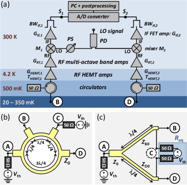
Figure 1: Schematics of the experimental setup (cf. main text). (a) Amplification and detection chains. (b) $180^{\circ}$ hybrid ring (HR). (c) Wilkinson power divider (WPD). For the WPD, port C represents a hidden internal port and $R_{\rm eq}$ an internal distributed resistor, which can be modeled as two equivalent matched $50\,\Omega$ loads adding correlated thermal noise via the hidden port C only.

As shown in Fig. 1(a), the output ports B and D of the beam splitter are connected to two symmetric amplification and detection chains, each comprising the following elements: (i) A cryogenic circulator at $500$ mK with 21 dB isolation which prevents amplifier noise from leaking back to the mw source under study. Furthermore, together with the isolation of two outputs of the beam splitters they avoid spurious correlations of the noise originating from the two amplification chains. (ii) A low-noise HEMT amplifier thermally anchored at $4.2$ K with power gain $G_{\rm HEMT}\simeq 24$ dB and noise temperature $T_{\rm HEMT}\simeq 6\pm 1$ K. The noise added by the linear HEMT amplifiers is the dominating amplifier noise in each detection channel and is expressed by $\hat{\chi}=V_{0}(\hat{\xi}^{{\dagger}}+\hat{\xi})$, where $\hat{\xi}^{{\dagger}}$ and $\hat{\xi}$ are bosonic creation and annihilation operators caves:1982:a . (iii) A room-temperature amplifier and (iv) a mixer (M) and local oscillator (LO) to down convert the mw signal to the intermediate frequency (IF). The phase $\varphi_{\rm LO}$ of one of the two LO signals obtained by means of a power divider (PD) can be varied by a phase shifter (PS). (v) An IF amplifier and (vi) a 7 kHz to 26 MHz band pass filter. Using a double sideband receiver the total bandwidth BW in our experiment is twice the bandwidth of the bandpass filter. The down converted voltage signal components $s_{1}$ and $s_{2}$ in the two chains are finally synchronously digitized by an acquisition board with $4\times 10^{8}$ samples/s and 12 bit resolution.

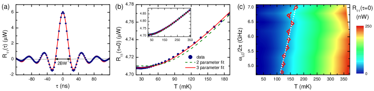
Figure 2: Planck spectroscopy of thermal mw states at $\omega/2\pi=5.3$ GHz using a WPD. (a) Auto-correlation function $R_{11}(\tau)$. The symbols represent the data, the line a fitted curve. (b) Temperature dependence of the variance $R_{11}(\tau{=}0)$ (Planck function). The symbols represent the data, the dotted and full lines are obtained by two and three parameter fits, respectively. The inset shows the data over a wider $T$ range. (c) Planck spectroscopy. Contour plot of $R_{11}(\tau=0)$ versus $T$ for different $\omega/2\pi$. The data has been corrected for the frequency dependent amplifier gain, the offset due to vacuum and amplifier noise has been subtracted. The symbols and the dashed line mark the experimentally measured and theoretically expected quantum crossover temperatures, respectively.

According to Nyquist nyquist:1928:a , the black body radiation emitted by a resistor with resistance $R_{0}$ within the bandwidth BW around the frequency $\omega=\omega_{\text{LO}}$ is given by $\langle V_{\rm th}^{2}\rangle/R_{0}=4\mathrm{BW}\langle n_{\rm th}\rangle\hbar\omega$. Here, $\langle n_{\rm th}\rangle$ is the average thermal photon population. It has been shown that for conductors with a large number of electronic modes the statistics of the emitted photons is given by a Bose-Einstein distribution beenacker:2001:a . In this case the well known result $\langle V_{\rm th}^{2}\rangle/R_{0}=4\mathrm{BW}\frac{\hbar\omega}{2}\coth(\hbar\omega/2k_{\rm B}T)$ is obtained. The power emitted into a perfectly matched circuit with characteristic impedance $Z_{0}$ is reduced by a factor of $1/4$ due to voltage division. Together with the beam splitter input/output relations of the HR, the signal components $s_{1}$ and $s_{2}$ are given by $s_{1}=\sqrt{G_{1}}(-\imath\alpha V^{A}_{\rm th}-\imath\beta V^{C}_{\rm th}+\chi_{1})$ and $s_{2}=\sqrt{G_{2}}(\imath\alpha V^{A}_{\rm th}-\imath\beta V^{C}_{\rm th}+\chi_{2})$. Here, $G_{1}\simeq G_{2}$ is the total power gain of the amplification chains, $\alpha=\beta=1/2\sqrt{2}$, and $\chi_{1}$ and $\chi_{2}$ are the independent noise contributions of the amplifiers. Equivalently, for the WPD we obtain $s_{1}=\sqrt{G_{1}}(-\imath\alpha V^{A}_{\rm th}+\imath\beta V^{C}_{\rm th}+\chi_{1})$ and $s_{2}=\sqrt{G_{2}}(-\imath\alpha V^{A}_{\rm th}-\imath\beta V^{C}_{\rm th}+\chi_{2})$. We note that $V^{A}_{\rm th}$, $V^{C}_{\rm th}$ and $\chi_{1,2}$ are classical realizations of the operators given above. By recording a large number of $1\mu$s-long time traces ($\sim 10^{6}$), the auto- and cross-correlation functions $R_{ii}(\tau)=\langle s^{\ast}_{i}(t+\tau)\,s_{i}(t)\rangle/Z_{0}=\sigma^{2}_{ii}\,{\rm sinc}({\rm BW}\,\tau)/Z_{0}$ and $R_{ij}(\tau)=\langle s^{\ast}_{i}(t+\tau)\,s_{j}(t)\rangle/Z_{0}=\sigma^{2}_{ij}\,{\rm sinc}({\rm BW}\,\tau)\,\cos\varphi_{\rm LO}/Z_{0}$, respectively, can be calculated ($i,j=1,2$). Since $\langle s_{i}(t)\rangle=0$ for thermal states, the auto- and cross-correlation functions are equal to the auto-variance $C_{ii}(\tau)=R_{ii}(\tau)-\langle s_{i}\rangle^{2}$ and cross-variance $C_{ij}(\tau)=R_{ij}(\tau)-\langle s_{i}\rangle\langle s_{j}\rangle$, respectively. Here, $\tau$ is the time shift between two traces being correlated, $\sigma^{2}_{ii}$ and $\sigma^{2}_{ij}$ are the variance and covariance of the voltage signals $s_{1}$ and $s_{2}$.

We first discuss the Planck spectroscopy experiment. Here, we use only a single amplification chain and determine the auto-correlation function $R_{11}(\tau)$ or $R_{22}(\tau)$. Exemplary, Fig. 2(a) shows the measured $R_{11}(\tau)$ curve obtained for $T=30$ mK using a WPD. A very similar result is obtained for $R_{22}(\tau)$ [see Fig. 3(d)]. Fitting the data to $C_{11}(\tau)$ allows us to extract the measurement bandwidth to ${\rm BW}\simeq 52$ MHz. Assuming that the signal contributions $V^{A}_{\rm th}$ and $V^{C}_{\rm th}$ due to the two load resistors and the noise $\chi_{i}$ of the HEMT amplifier are independent, we simply can add up their variances and obtain $R_{ii}(0)=C_{ii}(0)=\sigma^{2}_{ii}=\langle s_{i}^{2}\rangle/Z_{0}=\frac{G_{i}}{Z_{0}}\left[(\alpha^{2}+\beta^{2})\langle V^{2}_{\rm th}\rangle+\langle\chi^{2}_{i}\rangle\right]$. With $\hbar\omega/2k_{\rm B}T_{\rm HEMT}\ll 1$ we can introduce a classical noise temperature $T_{\rm i,HEMT}$ for the amplifiers and obtain

$$R_{ii}(0) = \;G^{\star}_{i}\;{\rm BW}\;\left[\frac{\hbar\omega}{2}\coth\frac{\hbar\omega}{2k_{\rm B}T}+k_{\rm B}T^{\star}_{\rm i,HEMT}\right]\,.$$ (1)

Here, $G^{\star}_{i}=\gamma G_{i}$ is the effective gain with $G_{i}$ the total gain of the amplification chain and $T^{\star}_{\rm i,HEMT}=T_{\rm i,HEMT}/\gamma$ is the amplifier effective noise temperature, representing the amplifier noise temperature relative to the input of the WPD. For both, the HR and WPD, $\gamma=4(\alpha^{2}+\beta^{2})=1$.

Figure 2(b) shows the measured variance $R_{11}(0)$ as a function of $T$ for $\omega/2\pi=5.3$ GHz in the case of a WPD. During the experiments, $T$ was varied between approximately $20$ and $350$ mK by means of a resistive heater and continuously monitored with a RuO thermometer. As expected, the measured variance is close to a Planck function and nicely reproduces the quantum crossover at $T_{\rm cr}=\hbar\omega/2k_{B}$. A fit of Eq. (1) to the data using $G^{\star}_{1}$ and $T^{\star}_{\rm 1,HEMT}$ as free parameters yields $G^{\star}_{1}\simeq 90$ dB and $T^{\star}_{\rm 1,HEMT}\simeq 6$ K. Evidently, there are slight deviations between the data and the two-parameter fit. This can be understood by taking into account that the effective electronic temperature $T_{\rm eff}$ of the load resistors at ports A and C may differ by a small amount $\delta T$. Using $\delta T$ as the third fitting parameter the solid line in Fig. 2(b) is obtained, demonstrating excellent agreement with the experimental data. The $\delta T$ values obtained by fitting the data are reasonably small and typically range between $1$ and $10$ mK. The large bandwidth of the HEMT amplifier allows us to perform equivalent measurements at several frequencies between $4.7$ and $7.1$ GHz. The result of such Planck spectroscopy is shown in Fig. 2(c). Clearly the quantum crossover temperature $T_{\rm cr}$ shifts to higher values with increasing frequency. Due to the finite uncertainty in $T_{\rm eff}$, we derive an effective crossover temperature $T_{\rm cr}+\delta T_{\rm cr}$ [cf. red crosses connected by a red line in Fig. 2(c)] which again slightly deviates from the theoretically expected value $T_{\rm cr}=\hbar\omega/2k_{\rm B}$ [cf. dashed white line in Fig. 2(c)]. The magnitude $\delta T_{\rm cr}$ quantifies the measurement fidelity $\mathcal{F}\equiv 1-|\delta T_{\rm cr}|/T_{\rm cr}$ of our setup for vacuum fluctuations. Notably, for the entire frequency range $\mathcal{F}\gtrsim 95$ %. In summary, our Planck spectroscopy experiments not only provide clear evidence for the Bose-Einstein statistics of photons emitted by a conductor in the few photon limit, but also directly demonstrate the frequency dependence of the quantum crossover temperature.

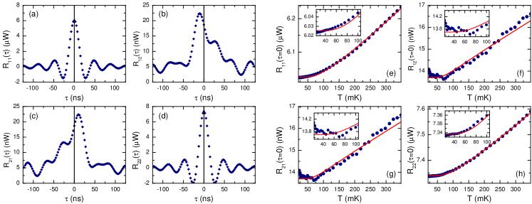
Figure 3: Full correlation function and covariance matrices measured at $\omega/2\pi=5.0$ GHz using a WPD ($G_{1}\simeq 90.5$ dB, $G_{2}\simeq 91.3$ dB, and $G_{12}\simeq 90.9$ dB. (a)–(d) $R_{ii}(\tau)$ and $R_{ij}(\tau)$ measured at $T=30$ mK. (e)–(h) Temperature dependence of $R_{ii}(0)$ and $R_{ij}(0)$. The symbols represent experimental data, the lines fits to the data.

We next turn to the analysis of the mw beam splitters. Figures 3(a)-3(d) show the entire correlation matrix. The off-diagonal elements are cross-correlation functions measured choosing $\varphi_{\rm LO}$ in order to obtain a maximum positive result. This guarantees that the signals associated with the two detection channels are skewed in phase and no unwanted de-correlation is introduced during the experiments. Since the signal contributions of the thermal noise sources and the amplifier noise are independent, all cross-correlations vanish, e.g. $\langle\hat{\chi}_{1}\hat{\chi}_{2}\rangle=\langle\hat{\chi}_{1}\rangle\langle\hat{\chi}_{2}\rangle=0$. Then, for $\alpha^{2}=\beta^{2}=1/8$ the covariance $R_{12}(0)=C_{12}(0)=\sigma_{12}^{2}$ is obtained to

$$R_{12}(0) = \frac{\hbar\omega}{4}G_{12}{\rm BW}\left[\coth\frac{\hbar\omega}{2k_{\rm B}T_{\rm A}}-\coth\frac{\hbar\omega}{2k_{\rm B}T_{\rm C}}\right]$$ (2)

with the power cogain $G_{12}=\sqrt{G_{1}}\sqrt{G_{2}}$. We note that the temperatures $T_{\rm A}$ and $T_{\rm C}$ of the load resistors at port A and C are identical only in the ideal case, resulting in $R_{12}(0)=0$ for the HR and WPD. However, in real experiments there may be small temperature differences $\delta T=T_{\rm A}-T_{\rm C}$. Figures 3(e)-3(h) show the covariance matrix as a function of $T$ for $\omega/2\pi=5.0$ GHz and using a WPD. The diagonal matrix elements $R_{11}(0)$ and $R_{22}(0)$ represent variance measurements and are analogous to the results of Fig. 2(b). The off-diagonal elements, instead, represent covariance measurements. It is evident that both the offset signal at 20 mK and the signal span between 20 and 350 mK for the covariance is reduced by about two orders of magnitude as compared to the variance. This suggests that there is a cancellation of both the amplifier noise and the signal when measuring the covariance. The former is due to the fact that the amplifier noises are uncorrelated. The latter is expected from Eq. (2). In order to prove this conjecture, we use Eq. (2) to fit the experimental data. Doing so we use the cogain which is determined by fitting the variance data. Furthermore, we set $T_{\rm A}=T$, where $T$ is the temperature measured by the thermometer, and use $\delta T$ as the free fitting parameter. In this way, we obtain the red curves in Figs. 3(f) and 3(g), which are in excellent agreement with the data. We obtain $\delta T$ values of a few mK. From the covariance measurements we can get information on the characteristics of the WPD. Since Eq. (2) explicitly assumes the existence of four ports, the perfect fit of the experimental data provides clear evidence that the WPD effectively behaves as a four-port device. In the quantum limit, this fourth port adds vacuum noise to any given input signal.

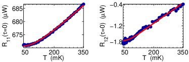
Figure 4: Temperature dependence of the (a) variance $R_{ii}(0)$ and (b) covariance $R_{ij}(0)$ measured at $\omega/2\pi=5.85$ GHz using a HR. The different power scale compared to Fig. 3(e)-(h) results from a different amplifier configuration.

In order to confirm our findings on the WPD, we have measured the $T$ dependence of the variance and covariance also for a HR (cf. Fig. 4), which is a straightforward four-port beam splitter. The covariance data of Fig. 4(b) are in excellent agreement with the fitted curve obtained from Eq. (2). This clearly demonstrates that, both the HR and WPD are characterized by the same fundamental quantum-mechanical behavior.

In conclusion, we have applied a correlation function analysis of the field quadratures to characterize black body radiation and the quantum properties of mw beam splitters. Our Planck spectroscopy experiments show that the mean thermal photon number emitted by a load resistor is following Bose-Einstein statistics and that the quantum crossover temperature shifts with frequency as $T_{\rm cr}=\hbar\omega/2k_{B}$, providing an indirect measure of mw vacuum fluctuations with high fidelity. Moreover, we have shown that, at the quantum level, vacuum fluctuations represent the minimum fundamental noise added by both three- and four-port microwave beam splitters.

This work is supported by the German Research Foundation through SFB 631, the German Excellence Initiative via NIM, NSERC, UPV-EHU GIU07/40, Ministerio de Ciencia e Innovación FIS2009-12773-C02-01, EU EuroSQIP and SOLID projects.

References

- (1) L. Mandel and E. Wolf, Optical Coherence and Quantum Optics (Cambridge Univ. Press, Cambridge, UK, 1995).
- (2) U. Leonhardt, Measuring the Quantum State of Light, (Cambridge Univ. Press, Cambridge, UK, 1997).
- (3) D. Bouwmeester, A. Ekert, and A. Zeilinger, The Physics of Quantum Information, (Springer-Verlag, Berlin, Germany, 2000).
- (4) P. Kok, W. J. Munro, K. Nemoto, T. C. Ralph, J. P. Dowling, and G. J. Milburn, Rev. Mod. Phys. 79, 135 (2007).
- (5) A. Wallraff et al., Nature 431, 162–167 (2004)
- (6) R. J. Schoelkopf and S. M. Girvin, Nature (London) 451, 664-669 (2008).
- (7) A. Blais et al., Phys. Rev. A 69, 062320 (2004).
- (8) O. Astafiev et al., Science 327, 840–843 (2010).
- (9) M. A. Sillanpää et al., Nature 449, 438 (2007).
- (10) J. Majer et al., Nature 449, 443 (2007).
- (11) A. A. Houck et al., Nature (London) 449, 328 (2007).
- (12) F. Deppe et al., Nature Physics 4, 686 (2008).
- (13) M. Mariantoni et al., Phys. Rev. B 78, 104508 (2008).
- (14) T. Niemczyk et al., Superc. Sci. Techn. 22, 034009 (2009).
- (15) D. Bozyigit et al., arXiv:1002.3738.
- (16) F. Helmer, M. Mariantoni, E. Solano, and F. Marquardt, Phys. Rev. A 79, 052115 (2009).
- (17) G. Romero, J. J. García-Ripoll, and E. Solano, Phys. Rev. Lett. 102, 173602 (2009).
- (18) E.P. Menzel et al., arxiv:1001.3669.
- (19) J. Gabelli et al., Phys. Rev. Lett. 93, 056801 (2004).
- (20) R. Movshovich et al., Phys. Rev. Lett. 65, 1419 (1990).
- (21) C.W.J. Beenakker and H. Schomerus, Phys. Rev. Lett. 86, 700 (2001).
- (22) R. E. Collin, Foundations for Microwave Engineering, 2nd ed., (Wiley-IEEE Press, New Jersey, 2000).
- (23) C. M. Caves, Phys. Rev. D 26, 1817 (1982).
- (24) H. Nyquist, Phys. Rev. 32, 110 (1928).