The early stages of star formation in Infrared Dark Clouds: characterizing the core dust properties

Abstract

Identified as extinction features against the bright Galactic mid-infrared background, infrared dark clouds (IRDCs) are thought to harbor the very earliest stages of star and cluster formation. In order to better characterize the properties of their embedded cores, we have obtained new 24 $\mu$m, 60–100 $\mu$m, and sub-millimeter continuum data toward a sample of 38 IRDCs. The 24 $\mu$m  Spitzer  images reveal that while the IRDCs remain dark, many of the cores are associated with bright 24 $\mu$m  emission sources, which suggests that they contain one or more embedded protostars. Combining the 24 $\mu$m, 60–100 $\mu$m, and sub-millimeter continuum data, we have constructed broadband spectral energy distributions (SEDs) for 157 of the cores within these IRDCs and, using simple gray-body fits to the SEDs, have estimated their dust temperatures, emissivities, opacities, bolometric luminosities, masses and densities. Based on their Spitzer/IRAC 3–8 $\mu$m  colors and the presence of 24 $\mu$m  point source emission, we have separated cores that harbor active, high-mass star formation from cores that are quiescent. The active ‘protostellar’ cores typically have warmer dust temperatures and higher bolometric luminosities than the more quiescent, perhaps ‘pre-protostellar’, cores. Because the mass distributions of the populations are similar, however, we speculate that the active and quiescent cores may represent different evolutionary stages of the same underlying population of cores. Although we cannot rule out low-mass star-formation in the quiescent cores, the most massive of them are excellent candidates for the ‘high-mass starless core’ phase, the very earliest in the formation of a high-mass star.

1 Introduction

The earliest phase of isolated low-mass star-formation occurs within Bok Globules. Viewed against background stars, Bok globules are identified as isolated, well-defined patches of optical obscuration and have typical visual extinctions, A_V, of 1–25 mag (Bok & Reilly, 1947). The individual precursor to a low-mass star, referred to as the ‘pre-protostellar core’, are found within Bok Globules. These pre-protostellar cores are typically small ($\sim$0.05 pc) and dense (10⁵–10⁶ ${\rm cm}^{-3}$), with low temperatures ($\sim$10 K) and low masses (0.5–5  $M_{\odot}$; e.g., Myers & Benson, 1983; Ward-Thompson et al., 1994).

Because many low-mass star-forming regions are nearby, their pre-protostellar cores and protostars have been studied extensively. Moreover, these studies have the added benefit of achieving sufficiently high spatial resolutions to distinguish the individual protostars, allowing one to study and characterize their various evolutionary stages, i.e., Class-0, I, II, and III (Lada & Wilking, 1984; Adams et al., 1987; Andre & Montmerle, 1994). These stages are characterized by IR spectral energy distributions (SEDs) corresponding to increasing black-body temperatures. Moreover, differences in the shapes of their SEDs trace the gradual removal of circumstellar material surrounding the central protostar as it evolves and emerges from its natal core.

While these early evolutionary stages are well-characterized for low-mass star-formation, it has been difficult to classify high-mass protostars in a similar manner. The combination of large distances to high-mass star-forming regions, their rarity and rapid evolution, and the fact that most high-mass stars form deeply embedded in dense molecular clumps and within clusters with many lower-mass stars nearby, makes their identification and separation difficult. However, in a recent study combining MSX, IRAS, and sub-millimeter data toward 42 regions of high-mass star formation, Molinari et al. (2008) have investigated the evolution of SEDs for young, high-mass protostars and has attempted to classify them via their SEDs. They find that objects in apparently different evolutionary stages occupy different areas in a bolometric luminosity versus envelope mass diagram, in a similar manner to the low-mass regime and, thus, conclude that high-mass star-formation may be a scaled up analog to low-mass star-formation. If this is the case, then perhaps the early stages of high-mass star-formation can also be characterized via differences in the SEDs of their dense molecular cores.

In order to better characterize the properties of high-mass pre-protostellar and protostellar cores, a large sample of cores in the very earliest stages of high-mass star-formation is required. High-mass stars and clusters form from cold, dense molecular clumps within giant molecular clouds (Blitz, 1991; Blitz & Williams, 1999; Lada & Lada, 2003). Recent studies suggest that the cold precursors of warm cluster-forming molecular clumps can be identified as ‘infrared dark clouds’ (IRDCs; Simon et al., 2006b; Rathborne et al., 2006). Surveys of the Galactic Plane at mid-IR wavelengths made with the ISO  and MSX  satellites first identified IRDCs as dark extinction features seen in absorption against the bright mid-IR emission arising from the Galactic background (Perault et al., 1996; Carey et al., 1998; Hennebelle et al., 2001). IRDCs are ubiquitous across the Galaxy (Simon et al., 2006a) and are typically long and very filamentary. They correspond to the densest parts of much larger giant molecular clouds (Simon et al., 2006b) and are characterized by high densities ($>10^{5}$ cm^-3), high column densities ($\sim$10²³–10²⁵ cm^-2), and low temperatures ($<25$ K; Egan et al., 1998; Carey et al., 1998, 2000).

Recently, Rathborne et al. (2006) conducted a survey of the 1.2 mm continuum emission toward 38 IRDCs using MAMBO-II on the IRAM 30 m telescope. These IRDCs were selected from the catalog of MSX  IRDC candidates (Simon et al., 2006a) and all have known kinematic distances, determined via the morphological match of ¹³CO(1–0)  emission to the mid-IR extinction (Simon et al., 2006b; Jackson et al., 2006). In these IRDCs Rathborne et al. (2006) found 190 cores, 140 of which are cold, compact cores. These cold, compact cores have typical sizes of $<$ 0.5 pc and masses of $\sim$ 120  $M_{\odot}$  (Rathborne et al., 2006). Indeed, millimeter and sub-millimeter observations toward other IRDCs suggest such compact cores are ubiquitous within IRDCs (e.g., Lis & Carlstrom, 1994; Carey et al., 2000; Garay et al., 2004; Ormel et al., 2005; Beuther et al., 2005). Because IRDCs are cold, their thermal dust emission will peak in the far-IR/sub-millimeter regime. At these wavelengths the dust emission is optically thin, making this regime the best for probing their internal structure and revealing their star-forming cores. If IRDCs are the high-mass analogue to Bok globules and the cold precursors to cluster-forming molecular clumps, then these dense cores may be the precursors to the stars (Rathborne et al., 2006).

IRAM and JCMT molecular line spectra, Spitzer  3–8 $\mu$m  and 24 $\mu$m  continuum images, and GBT water and methanol maser spectra toward a sample of cores within IRDCs reveal that most contain little evidence for active star-formation, such cores are called ‘quiescent’ (Chambers et al., 2009). However, some of the IRDC cores do appear to be actively forming stars as they show broad molecular line emission, shocked gas, bright 24 $\mu$m  emission, and strong water and methanol maser emission (e.g., Rathborne et al., 2005; Wang et al., 2006; Chambers et al., 2009). Each of these tracers provides independent evidence for star-formation, either indirectly (from the interaction between the protostar and the surrounding core traced through the broad line emission and the shocked gas) or more directly (from the heating of the dust surrounding the central protostar traced via the bright 24 $\mu$m  emission). It is likely, therefore, that these particular cores contain protostars. Indeed, a number of protostars have already been identified within IRDCs and span a range in mass, from low- and intermediate-mass (Carey et al., 2000; Redman et al., 2003) to high-mass (Beuther et al., 2005; Rathborne et al., 2005; Pillai et al., 2006; Wang et al., 2006).

In order to characterize the cores within IRDCs, we have conducted a large, multi-wavelength observational survey, combining IR, sub-millimeter, and millimeter continuum data. These data, when combined to make broadband SEDs, provide estimates of the core dust temperatures, dust emissivities, opacities, bolometric luminosities, and masses. Because the cores have SEDs that peak in the far-IR, to date, it has been very difficult to estimate bolometric luminosities of the individual protostars due to the uncertain extrapolation from much longer and/or shorter wavelengths. Indeed, many previous studies using MSX  and IRAS  fluxes have been forced to make assumptions about the relative contributions to the far-IR flux from individual objects within a star-forming region (e.g. Molinari et al., 2008). Thus, the inclusion of the sub-millimeter and far-IR data is critical to determine reliable SEDs for the cores and to better constrain these parameters. In this paper we provide the first mid-IR, far-IR, sub-millimeter, and millimeter SEDs for a large sample of cores within IRDCs.

2 Observations

The source list for these observations comprise 38 IRDCs and the 190 cores identified within them (Rathborne et al., 2006). To characterize the emission from these IRDCs and their cores, we have obtained continuum data at many wavelengths: 24 $\mu$m, 60–100 $\mu$m, 350 $\mu$m, 450 $\mu$m, 850 $\mu$m, and 1.2 mm. Table 1 gives a summary of the telescopes, instruments, wavelength range, observing dates, angular resolution and 1 $\sigma$ noise for the data.

2.1 24 $\mu$m  continuum images

The 24 $\mu$m  continuum images were obtained using the Multi-band Imaging Photometer (MIPS; Rieke et al., 2004) array on-board the Spitzer Space Telescope. Images toward 30 of the IRDCs were obtained as part of a Spitzer  cycle 1 General Observer (GO) proposal. The images were obtained in the raster-scanning mode during the periods 2004 October 16–19 and 2005 April 7–13. Because the IRDCs have complex and extended morphologies, the map sizes varied to cover the extent of the extinction at 8 $\mu$m. For 25 of the IRDCs, a 3 column $\times$ 3 row (13′$\times$13′) map was sufficient to cover the 8 $\mu$m  extinction. For four of the remaining IRDCs we used a 3 column $\times$ 5 row (13′$\times$19′) map, while toward the remaining IRDC, we used a 5 column $\times$ 5 row (19′$\times$ 19′) map to image the full extent of the 8 $\mu$m  extinction. In all cases, the raster map was stepped by half the array between consecutive scans. Three repeats of the map ($\sim$3 sec exposure time per point) were combined to produce the final image which achieved a 1 $\sigma$ point source sensitivity of 124 $\mu$Jy and an extended source sensitivity of 0.13 MJy sr^-1  (calculated using the on-line sensitivity calculator).

For the 8 IRDCs that were not part of our GO Spitzer  proposal, we use 24$\mu$m  images from MIPSGAL (see Carey et al., 2005 for a description of the survey details). These images were obtained by mapping large portions of the Galactic Plane using the ‘fast’ scanning mode. The resulting mosaics have a 1 $\sigma$ point source sensitivity of 207 $\mu$Jy and an extended source sensitivity of 0.21 MJy sr^-1.

All data were processed using the S13.2.0 version of the MIPS reduction pipeline.

2.2 60–100 $\mu$m  continuum spectra

We used the SED mode of Spitzer/MIPS to obtain long-slit, low-resolution (R$\sim$15–25) spectra toward a sample of these IRDC cores. Due to the saturation limits of MIPS toward the Galactic plane, our observations were limited to include only those cores with 1.2 mm fluxes $<$ 2 Jy. In total, we obtained a far-IR continuum spectrum toward 72 cores. For 65 of the cores, 4 repeats of a 10 sec integration were combined to produce the final spectrum which achieved a 1$\sigma$ sensitivity of $\sim$ 30, 70, and 150 mJy at 60, 75, and 90 $\mu$m  respectively. For the remaining 7 bright cores (those with 1.2 mm fluxes between 1–2 Jy), 4 repeats of a 3 sec exposure were combined. All spectra were obtained in the pointed observation mode. At these wavelengths, Spitzer  has an angular resolution of $\sim$13–24 ″  (9.8 ″ pixels).

Because of the contamination by the second order diffracted light and an inoperative detector module, the wavelength coverage of the spectra was restricted to 65–97 $\mu$m. The spectra were acquired in two epochs: 2006 October and 2007 May. Data from 2006 were processed using the S14.4.0 pipeline version, while 2007 data were reduced using version S16.1.0. The pointed SED-mode observation provides a set of six pairs of data frames between the target position (‘on’) and nearby sky position (‘off’). For all analysis, we use the pipeline produced post-basic calibrated data (post-BCDs), which deliver mosaic images for the ‘on’ and ‘off’ spectra.

We set the scan mirror to chop between the ‘on’ and ‘off’ positions with a chop throw of 1′  to 3′. The ‘off’ position was selected for each individual core to be nearby and free from 1.2 mm continuum emission. However, because the chop distance and visibility of the cores were limited, many of the ‘off’ positions fall within the 8 $\mu$m  extinction associated with the IRDC. Although the cores dominate, we found that many of the ‘off’ positions were not completely free of far-IR emission. Thus, we could not use the pipeline-produced ‘on-off’ spectra due to the ‘off’ contamination. Instead, we generated our own background and sky-subtracted spectrum using the local background immediately surrounding the core.

The spectra were flux calibrated using data obtained from multiple observations of three bright stars, with 70 $\mu$m  flux densities of 13–19 Jy. For point sources, the fluxes are accurate to within $\sim$ 20%. The typical 1 $\sigma$ noise in these data is $\sim$ 100 mJy beam^-1.

2.3 350 $\mu$m, 450 $\mu$m, and 850 $\mu$m  continuum images

The sub-millimeter continuum images were obtained using both the Caltech Submillimeter Observatory (CSO) and the James Clerk Maxwell Telescope (JCMT) via either a ‘scan-mapping’ or ‘on-the-fly’ mode. Due to weather and time constraints, not all 38 IRDCs were observed at all sub-millimeter wavelengths: in total, 37 of the IRDCs were observed at 350 $\mu$m, 29 at 450 $\mu$m  and 8 at 850 $\mu$m. All 350 $\mu$m  continuum images were obtained with the CSO and all 850 $\mu$m  continuum images were obtained with the JCMT. The 450 $\mu$m  continuum images were obtained at either the CSO or the JCMT.

The CSO data were obtained over three observing runs, 2004 September 5 and 9, 2005 April 12–15, and 2006 April 25–28 while the JCMT data were obtained on 2004 September 12–13. During the CSO observations, the $\tau_{\mathrm{225GHz}}$ measured from the CSO sky dipper was $\sim$ 0.07 during the 2005 and 2006 April observing periods and slightly higher, 0.09, for 2004 September. The measured 1 $\sigma$ noise in the images is $\sim$ 0.2 Jy beam^-1. The JCMT data were obtained in better conditions which resulted in a 1 $\sigma$ noise of $\sim$0.06 Jy beam^-1.

Where possible, the size of the individual maps were selected to cover the majority of the extinction feature and the 1.2 mm  continuum emission associated with the IRDC and ranged from 2′$\times$2′  to 8′$\times$8′. Standard reduction methods within the software packages CRUSH (for the CSO data) and SURF (for the JCMT data) were used to correct for atmospheric opacity and to remove atmospheric fluctuations. The data were flux-calibrated using either G34.3 or Uranus. Due to the uncertainties in accurate flux-calibration of sub-millimeter data, the calibration of the fluxes quoted here have errors of $\sim$ 40%.

3 Results

3.1 Continuum images

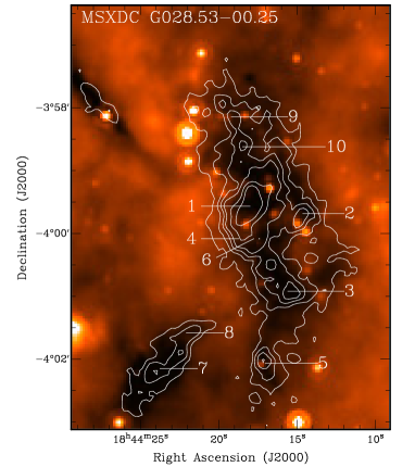
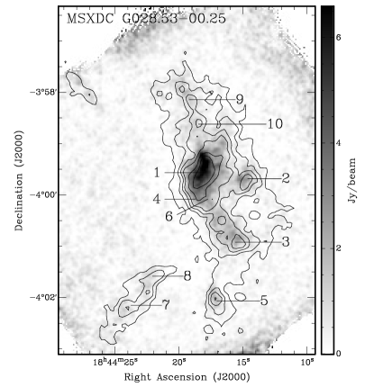
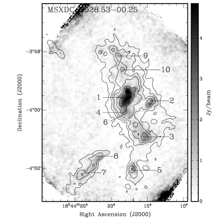
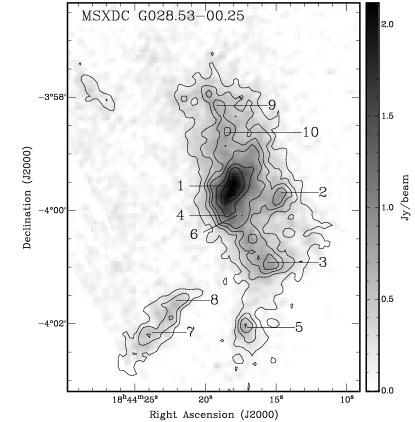
Figure 1: An example of the continuum data obtained toward the IRDC G028.53$-$00.25. From top left to bottom right the continuum images are: 24 $\mu$m, 350 $\mu$m, 450 $\mu$m, and 850 $\mu$m. In all cases the contours overlaid are the 1.2 mm continuum emission from Rathborne et al. (2006). The contour levels are 30 (3$\sigma$), 60, 90, 120, 180, 240 mJy beam^-1. These images reveal that while the IRDC remains dark at 24 $\mu$m  it is associated with bright emission at all sub-millimeter wavelengths. Moreover, the cores are clearly identified above the emission from the larger cloud. Broadband SEDs were generated for all the cores and their properties determined from gray-body fits. See the appendix for the SED plots and the derived parameters.

Figure 1 shows an example of the continuum data obtained toward one of the IRDCs: G028.53$-$00.25. Here we show the 24 $\mu$m, 850 $\mu$m, 450 $\mu$m, and 350 $\mu$m  continuum images overlaid with contours of the 1.2 mm continuum emission. The continuum data toward this IRDC is typical in that it shows that IRDCs remain dark at 24 $\mu$m, which confirms their extremely high column densities and low temperatures (see the appendix for all the 24 $\mu$m  images). Moreover, the 24 $\mu$m  extinction morphologies closely match the morphologies of the 1.2 mm continuum emission. This is expected as the 1.2 mm continuum emission traces the cold, dense dust which is blocking the Galactic mid-IR emission. While the IRDCs themselves remain dark, some IRDCs appear to contain bright, compact 24 $\mu$m  emission sources. In many cases these 24 $\mu$m  emission sources are coincident with the millimeter cores (e.g., Figs. A-4, A-7, A-9, A-25).

Sub-millimeter continuum emission was detected toward all the observed IRDCs and matches well the morphology of the 1.2 mm continuum emission (e.g.  Fig. 1). While the extended sub-millimeter continuum emission from the larger IRDC is sometimes faint, the cores are associated with bright, compact sub-millimeter continuum emission. Because strong emission at millimeter/sub-millimeter wavelengths can trace either temperature or column density enhancements, millimeter/sub-millimeter data alone are unable to accurately indicate the physical properties of potential star-forming cores. Thus, one needs an additional method to distinguish high temperature cores from high column density cores.

3.2 Spectral Energy Distributions

To characterize the emission arising from the cores, we have constructed broadband SEDs by combining the 24 $\mu$m, 60–100 $\mu$m, 350 $\mu$m, 450 $\mu$m, 850 $\mu$m, and 1.2mm continuum data. To model their SEDs we assume that the emission is optically thin and use a single temperature, modified gray-body function of the form,

$$F_{\nu}=\Omega_{s}\,B_{\nu}(T_{D})\,(1-e^{-\tau_{\nu}})$$

where $\Omega_{s}$  is the source solid angle, $B_{\nu}(T_{D})$ is the Planck function at the dust temperature ($T_{D}$), and $\tau_{\nu}$ is the optical depth (Gordon, 1995). We calculate $\tau_{250}$ using the relation $\tau_{\nu}=\tau_{250}(250/\lambda)^{\beta}$, where $\beta$ is the dust emissivity index and $\lambda$ is the wavelength in $\mu$m. The free parameters in the fits are the dust temperatures ($T_{D}$), optical depths at 250 $\mu$m  ($\tau_{250}$), and dust emissivity indices, $\beta$.

While this model may not be appropriate to characterize the emission in all cases, it is the simplest and most systematic approach we can take to obtaining estimates of the global dust parameters. Because we are interested in the entire core which is typically larger than protostellar envelopes and disks, this model will be sufficient and will produce a good approximation to the dust parameters on $\sim$ 1 pc spatial scales. Give the limited measurements at different wavelengths in the majority of the SEDs, complex radiation transfer modeling that includes disks, envelopes, protostars as well as several geometrical effects (e.g. Robitaille et al., 2007) would not produce robust results. Moreover, because the Robitaille et al. (2007) models currently do not incorporate the data at wavelengths $>$ 100 $\mu$m  accurately, the use of these detailed models is not appropriate for our purposes (priv. com. T. Robitaille).

The millimeter/sub-millimeter fluxes and sizes for each core were determined by fitting a two-dimensional gaussian profile with a constant background level to the emission at each core position (determined from the 1.2 mm continuum emission; see Table The early stages of star formation in Infrared Dark Clouds: characterizing the core dust properties and Rathborne et al., 2006). Each core was fit individually and the gaussian was inspected to determine that it fit well the flux from the core while excluding the underlying large-scale emission from the cloud.

The 24 $\mu$m  fluxes were calculated by interactively fitting a gaussian profile with a constant background level to the radial profile of the point source emission at each core position. This fitting takes into account any local variations in the noise of the data or variations in the local background emission. We assume an error for the 24 $\mu$m  flux calibration of 20%. In the majority of cases where a gaussian profile could not be fit to the emission, we have determined an upper limit to the flux by calculating the mean value in a small region centered at the core position. Because the emission may not be optically thin at 24 $\mu$m, the 24 $\mu$m  fluxes are only included in the SED fitting for cores that have no 60–100 $\mu$m  continuum spectrum. Because we wish to constrain the total luminosity of the core including any embedded sources, and the emission from the cores typically peaks in the far-IR, the 60–100 $\mu$m  data were crucial in determining a good fit, particularly in the cases where no 24 $\mu$m  emission was detected. For inclusion within the SED the 60–100 $\mu$m  continuum spectra were separated into 4 bins. The bin centers are at 55, 65, 75, 85, and 95 $\mu$m  and are 10 $\mu$m  wide. The mean fluxes within these ranges were used to produce the points that are included within the SEDs. Table The early stages of star formation in Infrared Dark Clouds: characterizing the core dust properties lists the coordinates, distances, and fluxes measured for all 190 cores.

A core SED was generated if fluxes could be extracted for at least two of the millimeter/sub-millimeter wavelengths. Thus, not all cores have an SED and derived parameters. We use the least squares fitting routine in IDL, MPFITFUN, to determine the best fit to the data. This procedure has the advantage of allowing us to constrain the values for the input parameters, include the errors in the fitting, and to correctly handle the upper limits at 24 $\mu$m. To model the gray-body emission we assume that the cores are isothermal and use a range in $T_{D}$ of 5–55 K, $\tau_{250}$ of 0.0001–1.0, and $\beta$ of 0.5–2.5. To account for the errors we assumed ’standard’ weighting for the data such that the weight, W = 1.0/error², where the error includes both the calibration uncertainty and the image noise, added in quadrature. When the core had a 24 $\mu$m  upper limit or a 60–100 $\mu$m  continuum spectrum, the weighting for the 24 $\mu$m  flux was set to 0.0 which forced the fitting routine to ignore this data point. In all of these cases the resulting fit was consistent with the upper limit (i.e. the function fell below the limit).

Figures A-1–A-32 show the 24 $\mu$m  image (overlaid with the 1.2 mm continuum emission) for each IRDC as well as the broadband SEDs for the cores. In total, broadband SEDs were generated for 157 of the sample of 190 cores. The millimeter/sub-millimeter/far-IR fluxes are shown on these plots as filled circles with the corresponding error bars. The 24 $\mu$m  fluxes are plotted as either filled circles (when included in the fitting), open circles (when excluded from the fitting), or as upper limit arrows.

For the 100 cores that have millimeter/sub-millimeter emission and either 24 $\mu$m  emission or a 60–100 $\mu$m  continuum spectrum, we plot the grey-body function (solid line) determined from the best fit. Labeled on each plot are the IRDC and core name, the output $T_{D}$, $\tau$, $\beta$, luminosity, mass and the $\chi^{2}$ returned from the fit. Using the output errors for the $T_{D}$, $\tau$, $\beta$, we also include the functions that correspond to the upper and lower values for the each of the three parameters (dotted lines). Table The early stages of star formation in Infrared Dark Clouds: characterizing the core dust properties lists the parameters determined for these cores.

The remaining 57 cores have an upper limit at 24 $\mu$m  and no 60–100 $\mu$m  continuum spectrum, i.e., only fluxes in the millimeter/sub-millimeter regime. Because the emission from the cores peaks in the far-IR, the absence of either a 24 $\mu$m  flux measurement or far-IR continuum spectrum made the determination of the individual core parameters difficult. For these cores the plots show two functions (examples are G015.31-00.16 MM4, MM5, G025.04-00.20 MM3, MM4, MM5; Figs. A-2 and  A-11 respectively). The first fit (solid line) is determined using only the millimeter/sub-millimeter fluxes. Because these SEDs only contain two data points and the emission likely does not cover the peak, the parameters determined from them are probably lower limits. The second fit (dashed line) was determined by including the 24 $\mu$m  upper limit as a real data point. In this case, the values determined from the fitting represent upper limits. For these cores we include two values for the $T_{D}$, $\tau$, $\beta$, luminosity, mass and $\chi^{2}$ on the plots; the estimated lower and upper limits. Table The early stages of star formation in Infrared Dark Clouds: characterizing the core dust properties lists the lower and upper limits to the parameters for these cores. Because these fits are unreliable the parameters derived from them are not included in any of the following analysis.

4 Discussion

4.1 Evidence for active star formation: separation of cores with high-mass protostars

To identify cores that may contain active star formation, we use a combination of their Spitzer /IRAC 3–8 $\mu$m  colors and the presence or absence of compact 24 $\mu$m  emission. We use the IRAC data and classification scheme presented in Chambers et al. (2009) but use our own 24 $\mu$m  flux measurements which were determined via a gaussian fit to the radial profile of the emission (rather than via aperture photometry as in Chambers et al., 2009).

The IRAC classification scheme is based on the colors of objects in the IRAC 3–8 $\mu$m  images which are grouped in to three categories: ‘red’, ‘green’, and ‘blue’. Most objects have either red or blue colors in these bands which indicate that that the flux is either increasing or decreasing, respectively, with wavelength. The ‘red’ objects are associated with bright 8 $\mu$m  emission and likely correspond to $\mathrm{H\,{\scriptstyle{II}}}$  regions while the ‘blue’ objects are associated with a region of bright 3.6 $\mu$m  emission and are predominantly unextincted stars. Those rare objects that are ‘green’ show enhanced emission at 4.5 $\mu$m  and could correspond to either an extincted star or, if the emission is extended, shocked gas. These latter objects are referred to as either ‘green fuzzies’ or EGOs (Chambers et al., 2009; Cyganowski et al., 2008), and are thought to trace the shocked gas in an outflow (Marston et al., 2004; Noriega-Crespo et al., 2004). Of the 190 cores within our sample, Chambers et al. (2009) find that 35 are associated with ‘red’, 47 with ‘green’, 6 with ‘blue’ objects, while the remaining 102 cores are not associated with any significant IRAC emission.

Emission at 24 $\mu$m  is an indicator of active star formation. Because this emission traces warm dust that is the heated as material accretes from a core onto a central protostar, the detection of a bright 24 $\mu$m  point source associated with a dense core suggests that star formation is occurring within it. We find that 93 of the 190 cores have a detectable 24 $\mu$m  point source emission.

Thus, the combination of a green fuzzy and 24 $\mu$m  emission toward a dense core suggests that there is both shocked gas and an accreting protostar within the core. Conversely, cores that do not contain an accreting protostar will remain cold, with dust temperatures too low to emit detectable 24 $\mu$m  emission. Because they also lack outflows, they will also show no evidence of shocked gas. As a result, the detection of a green fuzzy and a 24 $\mu$m  point source coincident with a core indicates active star formation within that core. Conversely, the non-detection of shocked gas and 24 $\mu$m  emission indicates that the core may be cold, with no (detectable) internal exciting source. While the absence of these star forming tracers is not definitive proof that there is no current star formation occurring within the core, it is suggestive. For example, low-mass protostars may lack sufficient luminosity to be detectable at 24 $\mu$m  given the typical distances to these IRDCs. However, a lack of heated dust and no shocked gas is certainly what is expected for a core in the cold, pre-protostellar phase.

Using their IRAC 3–8 $\mu$m  colors and their 24 $\mu$m  emission we use the Chambers et al. (2009) technique to separate the cores into five specific groups: quiescent cores, intermediate cores, active cores, red cores and blue cores. We define a ‘quiescent core’ to be a core that contains no significant 3–8 $\mu$m  nor 24 $\mu$m  emission. ‘Intermediate cores’ contain either a green fuzzy or a 24 $\mu$m  point source, but not both. ‘Active cores’ contain a green fuzzy and a 24 $\mu$m  point source. ‘Red cores’ are those cores associated with bright 8 $\mu$m  emission. Because bright emission at 8 $\mu$m  will be dominated by emission from either heated dust or UV-excited polycyclic aromatic hydrocarbons (PAHs), these cores likely correspond to embedded $\mathrm{H\,{\scriptstyle{II}}}$  regions where high-mass stars have already formed. Because the intermediate cores are associated with only one of the two proposed criteria for active star formation, we have separated these into a distinct group. These cores perhaps represent a transition phase between the active and quiescent cores.

Of the 190 cores, we group 35 as ‘red’, 6 as ‘blue’, 38 as ‘active’, 32 as ‘intermediate’, 79 as ‘quiescent’. We generated SEDs for 25 of the ‘red’, 3 of the ‘blue’, 34 of ‘active’, 29 of the ‘intermediate’, and 66 of the ‘quiescent’ cores. The IRAC classifications, the presence of 24 $\mu$m  emission and the resulting core designations are included on the SED plots.

4.2 Dust temperatures, opacities, and dust emissivities

Figures 2–4 show histograms for the number distributions of the derived T_D, $\tau_{250}$, and $\beta$ for our sample of cores. These figures are separated into four panels and show the number distributions for the red, active, intermediate, and quiescent cores for which reliable SEDs could be generated. For these 100 cores, 22 can be classified as ‘red’, 34 as ‘active’, 25 as ‘intermediate’, and 17 as ‘quiescent’. Table 2 lists the median and standard deviation measured from these distributions.

The derivation of core dust temperatures allows us to establish whether significant heating, either by accretion or embedded sources, is occurring within the cores (mean radius of $\sim$ 0.5 pc). As expected, Figure 2 shows that the highest dust temperatures are measured toward the red cores (median T_D of 41 K), which presumably already contain a high-mass star. The measured dust temperatures are cooler for the samples of active, intermediate, and quiescent cores (median of 34 K, 31 K and 23 K respectively) as expected if the star formation activity is in an earlier state.

While these dust temperatures are derived for each core individually, one must exercise caution when applying these temperatures to the cores where there is clearly active star formation. For instance, if the red cores really do harbor a high-mass star and $\mathrm{H\,{\scriptstyle{II}}}$  region, then close to the protostar their internal temperatures should be heated to well above 41 K. Because our angular resolution ($\sim$ 11″; 0.2 pc) samples dust from both the central protostar and its surrounding larger core, the derived dust temperatures reflect a beam-weighted average of the actual dust temperature distribution. If a cold $\sim$ 1 pc core contains a small volume of heated dust, the derived dust temperature will be larger than that of the cold envelope but smaller than that of the heated region. While the general trend of higher dust temperatures for cores with active star formation compared to lower temperatures for cores without star formation is expected, it is likely that, within the star-forming cores, there is a small volume of gas which is heated to temperatures significantly greater than those calculated here. Because the dust and gas are unlikely to be completely thermally coupled, it is possible that in these cases the gas temperatures are significantly higher than the dust temperatures derived from the SED fit.

The derived values of $\tau_{250}$ reveal that all cores are optically thin at 250 $\mu$m  ($\tau_{250}$ $\sim$ 0.01) regardless of their star-formation activity (Fig. 3). The derived values for $\beta$ (Fig. 4) show a range in values across the complete range input into the gray-body fitting routine. Since active star formation may change the properties of the dust grains, one might expect the emissivity index to vary between the different groups. It appears that, although they have fairly similar median values, the distributions may be slightly different for the red and active cores compared to the distribution for cores with no apparent star-formation.

4.3 Core masses, column and volume densities

Mass estimates obtained from molecular line emission toward very cold, very high column density cores are often unreliable. The combination of high molecular line optical depths toward these cores and the potential for molecular depletion makes it difficult to accurately trace the internal structure of such cores using molecular line emission. Because the emission from cold, dense dust peaks at millimeter/sub-millimeter wavelengths and is optically thin, it is a superior tracer of the internal structure and the masses of these cold, dense regions. However, accurate mass estimates from dust continuum emission require a good measurement of the dust temperatures and emissivities. Most mass estimates from dust emission assume a single value for $T_{D}$ and $\beta$. Because a large sample of cores potentially spans a large range in evolutionary stages and environments, the true values of $T_{D}$ and $\beta$ may vary considerably within the sample. To better determine the masses, therefore, one requires estimates of the dust temperatures and emissivities for each core. We have achieved this for our sample of cores and, thus, can now obtain a more accurate census of their masses, column and volume densities.

To calculate masses we use

$$M=\frac{F^{i}_{\nu}D^{2}}{\kappa_{\nu}B_{\nu}(T_{D})}$$

(Hildebrand, 1983), where $F^{i}_{\nu}$ is the observed integrated source flux density, $D$ is the distance, $\kappa_{\nu}$ is the dust opacity per gram of dust, and $B_{\nu}(T_{D})$ is the Planck function at the dust temperature. In all cases, we assume a gas-to-dust mass ratio of 100. We use the individual values for $T_{D}$ and $\beta$ derived from the SED for each core. To calculate the masses and densities we use the flux measured at 1.2 mm and $\kappa_{1.2mm}$ of 1.0 cm² g^-1 (Ossenkopf & Henning, 1994).

The beam-averaged H₂  column density, N(H₂), was calculated using the expression

$$N(H_{2})=\frac{F^{p}_{\nu}}{B_{\nu}(T_{D})\mu m_{p}\kappa_{\nu}\Omega_{b}}$$

where $F^{p}_{\nu}$ is the observed peak source flux density, $\mu$ is the mean molecular weight (2.8), $m_{p}$ is the mass of a proton, and $\Omega_{b}$ is the beam solid angle. The volume-averaged H₂  density, n(H₂), was estimated using the dust masses and by assuming a volume of a sphere. The derived masses, column and volume densities for the cores are listed in Table The early stages of star formation in Infrared Dark Clouds: characterizing the core dust properties.

Figures 5–7 show histograms of the number distributions for the masses, column and volume densities. A summary of the median and standard deviation values calculated from these distributions is given in Table 2. We find that the median masses are comparable between the red, active, intermediate, and quiescent cores (Fig. 5). To quantify the similarities between these distributions, we have also calculated, via a Kolmogorov-Smirnov (KS) test, the probability that these distributions arise from the same parent population. We find that the probability that the red and active cores are derived from the same parent is 6%, the probability that the red and quiescent cores are derived from the same parent is 84%, while the probability that the active and quiescent cores are derived from the same parent is 39%.

At all wavelengths the ‘active’ cores that show evidence for star formation activity have significantly more luminous emission compared to those that are more quiescent. However, such a close correspondence between the mass distributions of these populations implies that the bright emission observed toward the more active cores may simply arise from differences in their internal temperatures and not because they have higher densities. Indeed, we find no significant difference between the distribution for the derived column and volume densities for the cores that show star formation activity compared to those that are more quiescent (Figs. 6 and 7).

4.4 Core luminosities: identifying high-mass protostars and high-mass starless cores

Bolometric luminosities provide information on a core’s embedded young stellar objects and evolutionary state. The core luminosities were estimated by integrating the emission under the best fit gray-body curve and using the derived kinematic distance. The luminosities are included on the SED plot for each core and are listed in Table The early stages of star formation in Infrared Dark Clouds: characterizing the core dust properties.

Figure 8 shows the number distributions of the derived bolometric luminosities for the cores (the median and standard deviation values calculated from these distributions are given in Table 2). While the complete sample of cores span a range in bolometric luminosities of $\sim$10–10⁵  $L_{\odot}$, there is a clear trend for the core luminosity to decrease from the red cores to the quiescent cores. We find that the red cores have typical luminosities of $\sim$ 10^3.7  $L_{\odot}$, while the active and intermediate cores have lower luminosities of $\sim$ 10^2.8  $L_{\odot}$  and $\sim$ 10^2.3  $L_{\odot}$  respectively. Lower still, the quiescent cores have typical luminosities of $\sim$ 10^1.9  $L_{\odot}$.

A rough approximation of the final stellar mass can be made from the estimates of the core luminosity. Low-mass (M$<$2  $M_{\odot}$) stars never achieve luminosities $>$ 100  $L_{\odot}$  in their pre–main-sequence evolution (e.g.  Palla & Stahler, 1990). Because L $>$ 100  $L_{\odot}$  for the majority of the cores, it is unlikely that, in these cases, a single low-mass star dominates the core luminosity. Given our sensitivity and angular resolution, we cannot rule out the possibility, however, that many of the cores may comprise a cluster of unresolved low-mass stars that, together, produce a larger core luminosity.

On the other hand, high luminosities may arise because the core contains a high-mass protostar (M$>$8  $M_{\odot}$). Because the luminosity for a high-mass protostar ($\sim$10³–10⁵  $L_{\odot}$) is much larger than the luminosity from a low-mass protostar ($\sim$ 100  $L_{\odot}$), cores with luminosities $>$ 10⁴  $L_{\odot}$  probably harbor a high-mass protostar. Since high-mass stars typically form in clusters surrounded by many lower mass stars (Lada & Lada, 2003), lower mass protostars may also be forming within these cores and contributing to the overall observed luminosities. Regardless of the exact number of stars within the core, it is likely that the observed bolometric luminosity is dominated by the most massive protostar.

Using a bolometric luminosity of 10⁴  $L_{\odot}$  as a rough threshold, we can identify cores that have sufficient luminosities to harbor a high-mass protostar. When applying this threshold to the sample of ‘active’ and ‘intermediate’ cores, we find that 6 cores have luminosities $>$ 10⁴  $L_{\odot}$  and, thus, may contain a high-mass protostar (five from the active core sample and one from the intermediate core sample). Indeed, high-angular resolution millimeter/sub-millimeter interferometry images toward two of these cores (G024.33+00.11 MM1 and G034.43+00.24 MM; Figs. A-9 and A-25 respectively) show that both cores contain bright, compact structures that remain unresolved at $\sim$ 0.03 pc angular resolution (Rathborne et al., 2007, 2008). Moreover, their high-angular resolution spectra show many complex molecular emission features indicative of hot molecular cores (HMCs); an early stage in the formation of individual high-mass stars (e.g. Garay & Lizano, 1999).

The majority of the remaining active and intermediate cores (45 cores; 76%) have luminosities between 10² and 10⁴  $L_{\odot}$. If these cores contain a single protostar or main sequence star, then they likely correspond to an intermediate mass star (2 $<$ M $<$ 8  $M_{\odot}$). The active/intermediate cores that have lower bolometric luminosities (i.e. L $<$ 10²  $L_{\odot}$) may either be in an earlier evolutionary phase or be only forming low-mass protostars. They contain heated dust, as evidenced by the 24 $\mu$m  emission, but the current luminosity appears too low for a high-mass protostar. In these cases, the observed luminosity may arise from the accretion of material from the core onto the low-mass protostars. Indeed, recent work suggests low/intermediate mass protostars may continue to accrete material from their surroundings and grow to become high-mass protostars at the end of their evolution (e.g.  Beuther & Sridharan, 2007). Thus, we cannot rule out the possibility that these cores may eventually give rise to high-mass stars.

As expected, the quiescent cores all have lower (L$<$10³  $L_{\odot}$) bolometric luminosities, presumably because there is no high-mass central source to heat the dust. While the number of quiescent cores included within these histograms is small (17), there are 62 additional cores within these IRDCs that also meet our criteria for a lack of active, high-mass star formation. These cores have no detectable 3–8 $\mu$m  nor 24 $\mu$m  emission but do not have the far-IR continuum data which is invaluable for determining their properties. As a result, they are not included in the analysis here, but are also likely pre-protostellar in nature.

The quiescent cores have no apparent evidence for star-formation in the Spitzer  data. One possibility for this absence of star-formation activity is that they are young but will eventually form stars. On the other hand, it may be that these cores are currently forming only low-mass stars that are not bright enough to detect. Thus, we cannot rule out the possibility that the quiescent cores are currently forming low-mass protostars. Indeed, using the expression from the recent work of Krumholz & McKee (2008) that predicts the luminosity to mass ratio, L/M, of a core powered by the accretion on to low mass stars,

$$L/M=3.6M^{-0.33}\Sigma^{0.66}T_{b}^{0.16}\,L_{\odot}/M_{\odot}$$

where M is the core mass in units of 100  $M_{\odot}$, $\Sigma$  is the mass column density in g ${\rm cm}^{-2}$, and $T_{b}$ is the background temperature in units of 10 K, we find that for the quiescent cores, the median value predicted for the luminosity due to the accretion on to low-mass stars is $\sim$300  $L_{\odot}$. There are 6 quiescent cores within our sample that have luminosities comparable to, or greater than, 300  $L_{\odot}$. Thus, their observed luminosity could be powered by accretion onto low-mass stars.

At the distances to these IRDCs (typical distance of $\sim$ 4 kpc) low-mass protostars are difficult to detect. Thus, many of the ‘quiescent’ cores may contain low-mass protostars that will not be detectable with the available sensitivity and angular resolution. If, on the other hand, these candidate quiescent cores are in fact in a pre-protostellar phase, the most massive cores are excellent examples for the elusive ‘high-mass starless cores’; the very earliest stage in the formation of a high-mass star.

For the analysis presented in this paper, we assume that each core contains a single protostar. Without sensitive, high-angular resolution data, it is difficult to determine any potential multiplicity within the cores. High-angular resolution ($\sim$ 2″; $\sim$ 0.03 pc) millimeter and sub-millimeter data toward 6 of the highest mass cores within the current sample reveal that 4 of the cores are resolved into multiple protostellar condensations (Rathborne et al., 2007, 2008). It may be that these cores will in fact give rise to star clusters. In all cases, however, it appears that one central, massive condensation most likely dominates the bolometric luminosity.

Using the expression that relates the maximum stellar mass in a cluster ($m_{max}$) to the mass of the cluster ($M_{cluster}$), $m_{max}$ = 1.2 $M_{cluster}^{0.45}$ (Larson, 2003), we can estimate the mass of a cluster than will give rise to at least one high-mass star. Setting $m_{max}$ to 8  $M_{\odot}$, we find that the total cluster mass that will harbor a high-mass star should have a mass of $\sim$ 67  $M_{\odot}$. Assuming a cluster star formation efficiency of $\sim$ 30% (Lada & Lada, 2003), we calculate that such a stellar cluster could form from a core with a mass of $\sim$ 225  $M_{\odot}$. Thus, in the pre-protostellar phase, a core that will form a star cluster that will eventually form a high-mass star ought to have a mass of at least $\sim$ 225  $M_{\odot}$. Five quiescent cores within these IRDCs meet this criteria and, thus, will probably form a cluster with a high-mass star. In particular, the most massive of these, the cores G028.53$-$00.25 MM1 and MM3 (Fig. A-7) have low dust temperatures ($\sim$ 20 K) and bolometric luminosities ($\sim$ 10²  $L_{\odot}$), but high masses ($\sim$ 10³  $M_{\odot}$), column densities ($\sim$ 6$\times 10^{23}$  ${\rm cm}^{-2}$) and volume densities ($\sim$ 10⁶ ${\rm cm}^{-3}$). These values are consistent with the expected properties of high-mass starless cores.

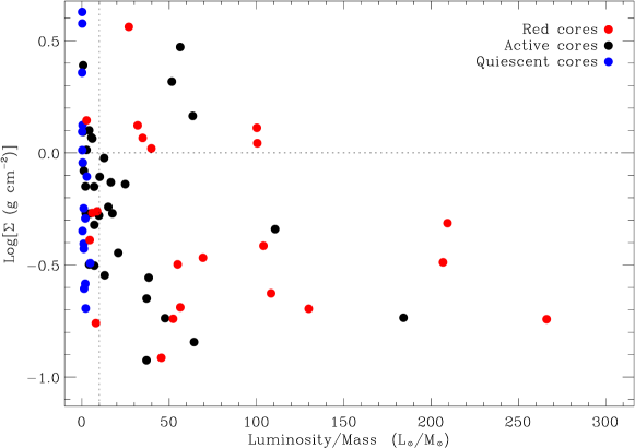
Figure 9: Plot of bolometric luminosity to mass ratio (L/M) versus mass column density ($\Sigma$) for the cores. The dotted lines mark the critical values of these parameters for the formation of a high-mass star (determined from the recent theoretical work of Krumholz & McKee, 2008). These criteria mark the thresholds above which the fragmentation of a core is suppressed, by the increase in temperature and Jeans mass. According to these criteria, we find that nine of the cores may give rise to a high-mass protostar. For the remaining cores, it appears that the fragmentation and the formation of lower-mass protostars is still possible.

Recent theoretical work suggests that to form a high-mass star from a core the cloud’s critical mass column density, $\Sigma$, should be $\gtrsim$ 1 g cm^-2 and its luminosity-to-mass ratio, L/M, $\gtrsim$ 10  $L_{\odot}$/ $M_{\odot}$  (Krumholz & McKee, 2008). Under these conditions, further fragmentation is suppressed by accretion onto nearby lower-mass protostars and the subsequent heating of the surrounding material. It is thought that an increase in temperature to $\sim$ 100 K is sufficient to increase the Jeans mass and, thus, halt the fragmentation process. Figure 9 plots L/M versus $\Sigma$ for our sample of cores, with these thresholds overlaid.

We find that 6 red cores and 3 active cores have L/M $>$ 10  $L_{\odot}$/ $M_{\odot}$  and $\Sigma$ $>$ 1 g ${\rm cm}^{-2}$  and, thus, have sufficient luminosity and mass to form a high-mass protostar (according to the Krumholz & McKee, 2008 criteria). For the remaining cores, it appears that the fragmentation and the formation of lower-mass protostars is still possible. If these conditions hold, then these cores may be resolved into multiple protostellar condensations in high-angular resolution data. Because the size scales of these cores are $\sim$ 0.5 pc and are comparable to the size scales over which a star cluster may form rather than the individual stars, it is unclear if these criteria are applicable. However, their low $\Sigma$ is consistent with the fact that they will likely fragment further.

4.5 Evolutionary sequence

The combination of data sets spanning wavelengths from the millimeter through the sub-millimeter and far-IR allows us to investigate the differences between the cores that show evidence for high-mass star formation activity from those that are more quiescent. Because we can derive both masses and temperatures from the data, we can separate their effects. One hypothetical possibility is that the core properties merely reflect an evolutionary sequence. If this idea is correct, then the colder ‘quiescent’ cores are pre-protostellar and will evolve into the warmer, ‘active’ protostellar cores as protostars form within them and begin to heat them internally. In this case, only the temperature of the cores should vary, since the mass for the entire cluster-forming core is unlikely to change very much as it evolves. Thus, one would expect the active cores to be warmer than the quiescent cores, but that their mass distributions should be the same.

An alternative possibility is that the cores that show evidence for star-formation simply contain more luminous, high-mass protostars, whereas the more quiescent cores contain only lower mass protostars. Thus, the lack of obvious star-formation activity in the quiescent cores would then result from the difficulty to detect the much fainter lower-mass protostars. Since low-mass stars form from lower-mass cores, in this scenario, one would expect the quiescent cores to have both lower temperatures and smaller masses on average than the active cores. Thus, the data allow us to distinguish between these two competing ideas: evolution and mass.

While the derived dust temperatures and luminosities are higher for the cores that show evidence for star-formation compared to those that are more quiescent, the mass distributions for the two populations are similar. In fact, the KS test shows that the probability that the active and quiescent cores are derived from the same parent population is $\sim$40%. The similarity in their mass distributions suggests that the underlying populations are nearly the same, and that the differences in their temperature and luminosity reflect different evolutionary stages. If this is the case, then the quiescent cores have enough mass to form a high-mass protostar, however, they simply have not yet begun the process. Such cores should still be cold, and since no high-mass protostars have formed yet, also have low bolometric luminosities. In contrast, the active cores contain an internal protostellar heating source(s) which results in their higher dust temperatures and luminosities.

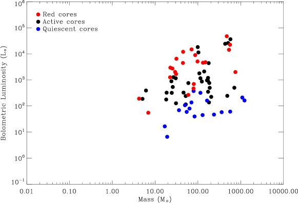
Figure 10: Plot of bolometric luminosity versus mass for the cores. We find that for a given mass the luminosity increases from the quiescent, to the active, to the red cores. This is consistent with the idea that the quiescent cores are in an earlier evolutionary phase compared to the active and red cores.

The evolutionary differences between the samples of cores can also be seen in a bolometric luminosity versus core dust mass diagram (e.g., Fig. 10; Sridharan et al., 2002; Molinari et al., 2008). For both the low- and high-mass regimes, sources in different evolutionary phases have been shown to lie in distinct regions within this diagram. As the protostellar activity increases, the luminosity also increases such that the different stages within the star formation process occupy regions that overlap in mass but are offset to higher luminosities. Similar to the results of Molinari et al. (2008), we find that these IRDC cores lie in the high-mass regime and that, for a given mass, the bolometric luminosities increase from the quiescent, to the active cores, to the red cores. This is consistent with the idea that the quiescent cores are in an earlier evolutionary phase compared to the active and red cores.

5 Conclusions

To characterize the physical properties of cores within IRDCs we have obtained new 24 $\mu$m, 60–100 $\mu$m, and sub-millimeter continuum data toward a sample of 38 IRDCs. These IRDCs contain 190 compact cores, 140 of which are dark at 8 $\mu$m  and are cold, compact and dense. The Spitzer/MIPS 24 $\mu$m  images reveal that while the IRDCs remain dark, many of their cores are associated with bright 24 $\mu$m  emission sources. The sub-millimeter continuum data elucidate both the large- and small-scale structure of the IRDCs. Because emission at millimeter/sub-millimeter wavelengths can trace either temperature and/or density enhancements one needs an additional method to distinguish between these two parameters. Using the presence or absence of 24 $\mu$m  point source emission, in combination with their Spitzer/IRAC 3–8 $\mu$m  colors, we have classified the cores into five groups: red, active, intermediate, quiescent, and blue. We find that, of the 190 cores, 35 can be classified as red, 38 as active, 32 as intermediate, 79 as quiescent, and 6 as blue.

From gray-body fits to their spectral energy distributions (SEDs) we have determined the dust temperatures, emissivities, opacities, bolometric luminosities, and masses for a large sample of the IRDC cores. The derived distributions of the dust temperatures, luminosities, and masses for the different groups of cores reveals that the dust temperatures and luminosities are higher for those cores that show active, high-mass star formation compared to those cores that are more quiescent. Lower dust temperatures and luminosities are expected for the quiescent cores because they presumably have no high-mass internal source to significantly heat the dust. Comparing the derived masses for the core samples, however, we find that their mass distributions are similar. We interpret this similarity to be a result of evolutionary differences: the cooler quiescent cores may be the pre-protostellar precursors to the warmer, more active protostellar cores.

Using their derived bolometric luminosities, we estimate that $\sim$10% of the cores that show evidence for star formation may contain high-mass protostars. If the quiescent cores are indeed devoid of star formation, then the most massive of these are excellent candidates for the ‘high-mass starless core’ phase, a very early phase in the formation of a high-mass star. Because of their distances, we cannot yet rule out the possibility that many of these cores may contain low-mass stars. Observations with ALMA will be crucial to address this issue. Nevertheless, our study supports the idea that IRDCs harbor the very earliest evolutionary stages in the formation of high-mass stars and, thus, clusters.

Appendix

Figures A-1–A-32 show the 24 $\mu$m  image toward the IRDCs overlaid with the 1.2 mm continuum emission. Also included in these figures are the SEDs and gray-body fits for each of the cores that had sufficient data. Table The early stages of star formation in Infrared Dark Clouds: characterizing the core dust properties list the coordinates, distances, and fluxes measured toward all cores. Marked on the SEDs and listed in Table The early stages of star formation in Infrared Dark Clouds: characterizing the core dust properties and Table The early stages of star formation in Infrared Dark Clouds: characterizing the core dust properties are the derived parameters.

Table 1: Summary of the observations.

Telescope	Instrument	Wavelength	Date	Angular	1 $\sigma$
				Resolution	sensitivity
Spitzer  0.85 m	MIPS	24 $\mu$m	2004 Oct, 2005 Apr	6 ″	$\sim$150 $\mu$Jy
Spitzer  0.85 m	SED-mode	60–100 $\mu$m	2006 Oct, 2007 May	13–24 ″	$\sim$100 mJy
CSO 10 m	SHARC-2	350, 450 $\mu$m	2005 Sept, 2005 Apr, 2006 Apr	8 ″	$\sim$ 200 mJy
JCMT 15 m	SCUBA	450, 850 $\mu$m	2004 Sept	8, 15 ″	$\sim$ 60 mJy
IRAM 30 m	MAMBO-II	1.2 mm	2004 Feb	11 ″	$\sim$ 10 mJy

Table 2: Summary of the derived core properties

Property	Red		Active		Intermediate		Quiescent
	Median	Stddev	Median	Stddev	Median	Stddev	Median	Stddev
TD (K)	40.4	5.7	34.5	6.5	30.4	8.1	23.7	5.3
Log[$\tau_{250}$]	-1.894	0.575	-2.081	0.550	-2.456	0.628	-2.404	0.501
$\beta$	1.7	0.4	1.6	0.4	1.4	0.5	1.2	0.5
Log[Mass] ( $M_{\odot}$)	1.85	0.59	2.06	0.54	1.97	0.61	1.92	0.55
Log[Lum] ( $L_{\odot}$)	3.65	0.72	2.88	0.69	2.27	0.79	1.84	0.44
$\Sigma$ (g ${\rm cm}^{-2}$)	-0.39	0.39	-0.15	0.34	-0.29	0.42	-0.25	0.40
Log[N(H2)] (${\rm cm}^{-2}$)	22.05	0.42	22.10	0.43	22.03	0.36	22.01	0.29
Log[n(H2)] (${\rm cm}^{-3}$)	5.82	0.38	5.98	0.32	5.81	0.42	6.06	0.39

Figure 2: Histograms of the dust temperature (T_D) derived from the gray-body fits to the core SEDs. The panels shows the histograms for the samples of the red, active, intermediate, and quiescent cores. We find that, as expected, the derived dust temperatures decrease from the red, to the active, to the intermediate, to the quiescent cores. Table 2 lists the median and standard deviations of these distributions.

Figure 3: Histograms of the 250 $\mu$m  opacity ($\tau_{250}$) derived from the gray-body fits to the core SEDs. The panels show the histograms for the samples of the red, active, intermediate, and quiescent cores. We find that the majority of the cores are optically thin, with low values of $\tau_{250}$ (most have $\tau_{250}<$ 0.01). Table 2 lists the median and standard deviations of these distributions.

Figure 4: Histograms of the dust emissivity index ($\beta$) derived from the gray-body fits to the core SEDs. The panels show the histograms for the samples of the red, active, intermediate, and quiescent cores. Although they span a similar range, the median of the distribution of $\beta$ for star-forming cores may be different from the median of the distribution of $\beta$ for cores with no apparent star-formation . Table 2 lists the median and standard deviations of these distributions.

Figure 5: Histograms of the derived dust mass. The panels show the histograms for the samples of the red, active, intermediate, and quiescent cores. We find that the mass distributions for the cores span a similar range, regardless of their apparent star-formation activity. Table 2 lists the median and standard deviations of these distributions.

Figure 6: Histograms of the derived H₂  column density, N(H₂). The panels show the histograms for the samples of the red, active, intermediate, and quiescent cores. We find that the cores have similar column densities, regardless of their apparent star-formation activity. Table 2 lists the median and standard deviations of these distributions.

Figure 7: Histograms of the derived H₂  volume density, n(H₂). The panels show the histograms for the samples of the red, active, intermediate, and quiescent cores. We find that the cores have similar volume densities, regardless of their apparent star-formation activity. Table 2 lists the median and standard deviations of these distributions.

Figure 8: Histograms of the bolometric luminosity derived from the gray-body fits to the core SEDs. The panels show the histograms for the samples of the red, active, intermediate, and quiescent cores. We find that, as expected, the derived luminosities decrease from the red, to the active, to the intermediate, to the quiescent cores. Table 2 lists the median and standard deviations of these distributions.

Figure A-1: Spitzer  24 $\mu$m  image overlaid with 1.2 mm continuum emission for G015.05+00.07  (contour levels are 30 and 60 mJy beam^-1). The lower panels show the broadband SEDs for cores within this IRDC. The fluxes derived from the millimeter, sub-millimeter, and far-IR continuum data are shown as filled circles (with the corresponding error bars), while the 24 $\mu$m  fluxes are shown as either a filled circle (when included within the fit), an open circle (when excluded from the fit), or as an upper limit arrow. For cores that have measured fluxes only in the millimeter/sub-millimeter regime (i.e.  a limit at 24 $\mu$m), we show the results from two fits: one using only the measured fluxes (solid line; lower limit), while the other includes the 24 $\mu$m  limit as a real data (dashed line; upper limit). In all other cases, the solid line is the best fit gray-body, while the dotted lines correspond to the functions determined using the errors for the T_D, $\tau$, and $\beta$ output from the fitting. Labeled on each plot is the IRDC and core name, classification, and the derived parameters.

Figure A-2: Spitzer  24 $\mu$m  image overlaid with 1.2 mm continuum emission for G015.31$-$00.16  (contour level is 30 mJy beam^-1). The lower panels show the broadband SEDs for cores within this IRDC. The fluxes derived from the millimeter, sub-millimeter, and far-IR continuum data are shown as filled circles (with the corresponding error bars), while the 24 $\mu$m  fluxes are shown as either a filled circle (when included within the fit), an open circle (when excluded from the fit), or as an upper limit arrow. For cores that have measured fluxes only in the millimeter/sub-millimeter regime (i.e.  a limit at 24 $\mu$m), we show the results from two fits: one using only the measured fluxes (solid line; lower limit), while the other includes the 24 $\mu$m  limit as a real data (dashed line; upper limit). In all other cases, the solid line is the best fit gray-body, while the dotted lines correspond to the functions determined using the errors for the T_D, $\tau$, and $\beta$ output from the fitting. Labeled on each plot is the IRDC and core name, classification, and the derived parameters.

Figure A-3: Spitzer  24 $\mu$m  image overlaid with 1.2 mm continuum emission for G018.82$-$00.28  (contour levels are 30, 60, 90, 120, 240 mJy beam^-1). The lower panels show the broadband SEDs for cores within this IRDC. The fluxes derived from the millimeter, sub-millimeter, and far-IR continuum data are shown as filled circles (with the corresponding error bars), while the 24 $\mu$m  fluxes are shown as either a filled circle (when included within the fit), an open circle (when excluded from the fit), or as an upper limit arrow. For cores that have measured fluxes only in the millimeter/sub-millimeter regime (i.e.  a limit at 24 $\mu$m), we show the results from two fits: one using only the measured fluxes (solid line; lower limit), while the other includes the 24 $\mu$m  limit as a real data (dashed line; upper limit). In all other cases, the solid line is the best fit gray-body, while the dotted lines correspond to the functions determined using the errors for the T_D, $\tau$, and $\beta$ output from the fitting. Labeled on each plot is the IRDC and core name, classification, and the derived parameters.

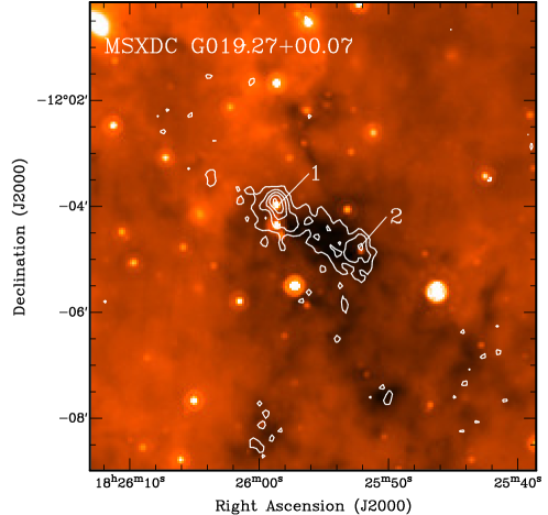
Figure A-4: Spitzer  24 $\mu$m  image overlaid with 1.2 mm continuum emission for G019.27+00.07  (contour levels are 30, 60, 90, 120, 240 mJy beam^-1). The lower panels show the broadband SEDs for cores within this IRDC. The fluxes derived from the millimeter, sub-millimeter, and far-IR continuum data are shown as filled circles (with the corresponding error bars), while the 24 $\mu$m  fluxes are shown as either a filled circle (when included within the fit), an open circle (when excluded from the fit), or as an upper limit arrow. For cores that have measured fluxes only in the millimeter/sub-millimeter regime (i.e.  a limit at 24 $\mu$m), we show the results from two fits: one using only the measured fluxes (solid line; lower limit), while the other includes the 24 $\mu$m  limit as a real data (dashed line; upper limit). In all other cases, the solid line is the best fit gray-body, while the dotted lines correspond to the functions determined using the errors for the T_D, $\tau$, and $\beta$ output from the fitting. Labeled on each plot is the IRDC and core name, classification, and the derived parameters.

Figure A-5: Spitzer  24 $\mu$m  image overlaid with 1.2 mm continuum emission for G022.35+00.41  (contour levels are 30, 60, 90, 120, 240 mJy beam^-1). The lower panels show the broadband SEDs for cores within this IRDC. The fluxes derived from the millimeter, sub-millimeter, and far-IR continuum data are shown as filled circles (with the corresponding error bars), while the 24 $\mu$m  fluxes are shown as either a filled circle (when included within the fit), an open circle (when excluded from the fit), or as an upper limit arrow. For cores that have measured fluxes only in the millimeter/sub-millimeter regime (i.e.  a limit at 24 $\mu$m), we show the results from two fits: one using only the measured fluxes (solid line; lower limit), while the other includes the 24 $\mu$m  limit as a real data (dashed line; upper limit). In all other cases, the solid line is the best fit gray-body, while the dotted lines correspond to the functions determined using the errors for the T_D, $\tau$, and $\beta$ output from the fitting. Labeled on each plot is the IRDC and core name, classification, and the derived parameters.

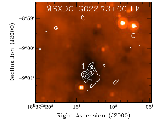
Figure A-6: Spitzer  24 $\mu$m  image overlaid with 1.2 mm continuum emission for G022.73+00.11  (contour levels are 20, 30 and 45 mJy beam^-1). The lower panels show the broadband SEDs for cores within this IRDC. The fluxes derived from the millimeter, sub-millimeter, and far-IR continuum data are shown as filled circles (with the corresponding error bars), while the 24 $\mu$m  fluxes are shown as either a filled circle (when included within the fit), an open circle (when excluded from the fit), or as an upper limit arrow. For cores that have measured fluxes only in the millimeter/sub-millimeter regime (i.e.  a limit at 24 $\mu$m), we show the results from two fits: one using only the measured fluxes (solid line; lower limit), while the other includes the 24 $\mu$m  limit as a real data (dashed line; upper limit). In all other cases, the solid line is the best fit gray-body, while the dotted lines correspond to the functions determined using the errors for the T_D, $\tau$, and $\beta$ output from the fitting. Labeled on each plot is the IRDC and core name, classification, and the derived parameters.

Figure A-7: Spitzer  24 $\mu$m  image overlaid with 1.2 mm continuum emission for G023.60+00.00  (contour levels are 30, 60, 90, 120, 240, 360, 480 mJy beam^-1). The lower panels show the broadband SEDs for cores within this IRDC. The fluxes derived from the millimeter, sub-millimeter, and far-IR continuum data are shown as filled circles (with the corresponding error bars), while the 24 $\mu$m  fluxes are shown as either a filled circle (when included within the fit), an open circle (when excluded from the fit), or as an upper limit arrow. For cores that have measured fluxes only in the millimeter/sub-millimeter regime (i.e.  a limit at 24 $\mu$m), we show the results from two fits: one using only the measured fluxes (solid line; lower limit), while the other includes the 24 $\mu$m  limit as a real data (dashed line; upper limit). In all other cases, the solid line is the best fit gray-body, while the dotted lines correspond to the functions determined using the errors for the T_D, $\tau$, and $\beta$ output from the fitting. Labeled on each plot is the IRDC and core name, classification, and the derived parameters.

Figure A-8: Spitzer  24 $\mu$m  image overlaid with 1.2 mm continuum emission for G024.08+00.04  (contour levels are 30, 60, 90, 120, 240 mJy beam^-1). The lower panels show the broadband SEDs for cores within this IRDC. The fluxes derived from the millimeter, sub-millimeter, and far-IR continuum data are shown as filled circles (with the corresponding error bars), while the 24 $\mu$m  fluxes are shown as either a filled circle (when included within the fit), an open circle (when excluded from the fit), or as an upper limit arrow. For cores that have measured fluxes only in the millimeter/sub-millimeter regime (i.e.  a limit at 24 $\mu$m), we show the results from two fits: one using only the measured fluxes (solid line; lower limit), while the other includes the 24 $\mu$m  limit as a real data (dashed line; upper limit). In all other cases, the solid line is the best fit gray-body, while the dotted lines correspond to the functions determined using the errors for the T_D, $\tau$, and $\beta$ output from the fitting. Labeled on each plot is the IRDC and core name, classification, and the derived parameters.

Figure A-9: Spitzer  24 $\mu$m  image overlaid with 1.2 mm continuum emission for G024.33+00.11  (contour levels are 30, 60, 90, 120, 240, 360, 480, 840, 1200 mJy beam^-1). The lower panels show the broadband SEDs for cores within this IRDC. The fluxes derived from the millimeter, sub-millimeter, and far-IR continuum data are shown as filled circles (with the corresponding error bars), while the 24 $\mu$m  fluxes are shown as either a filled circle (when included within the fit), an open circle (when excluded from the fit), or as an upper limit arrow. For cores that have measured fluxes only in the millimeter/sub-millimeter regime (i.e.  a limit at 24 $\mu$m), we show the results from two fits: one using only the measured fluxes (solid line; lower limit), while the other includes the 24 $\mu$m  limit as a real data (dashed line; upper limit). In all other cases, the solid line is the best fit gray-body, while the dotted lines correspond to the functions determined using the errors for the T_D, $\tau$, and $\beta$ output from the fitting. Labeled on each plot is the IRDC and core name, classification, and the derived parameters.

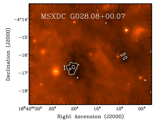
Figure A-10: Spitzer  24 $\mu$m  image overlaid with 1.2 mm continuum emission for G024.60+00.08  (contour levels are 30, 60, 90, 120, 240, 360, 480, 840, 1200 mJy beam^-1). The lower panels show the broadband SEDs for cores within this IRDC. The fluxes derived from the millimeter, sub-millimeter, and far-IR continuum data are shown as filled circles (with the corresponding error bars), while the 24 $\mu$m  fluxes are shown as either a filled circle (when included within the fit), an open circle (when excluded from the fit), or as an upper limit arrow. For cores that have measured fluxes only in the millimeter/sub-millimeter regime (i.e.  a limit at 24 $\mu$m), we show the results from two fits: one using only the measured fluxes (solid line; lower limit), while the other includes the 24 $\mu$m  limit as a real data (dashed line; upper limit). In all other cases, the solid line is the best fit gray-body, while the dotted lines correspond to the functions determined using the errors for the T_D, $\tau$, and $\beta$ output from the fitting. Labeled on each plot is the IRDC and core name, classification, and the derived parameters.

Figure A-11: 3 Spitzer  24 $\mu$m  image overlaid with 1.2 mm continuum emission for G025.04$-$00.20  (contour levels are 30, 60, 90, 120, 240, 360, 480, 840, 1200 mJy beam^-1). The lower panels show the broadband SEDs for cores within this IRDC. The fluxes derived from the millimeter, sub-millimeter, and far-IR continuum data are shown as filled circles (with the corresponding error bars), while the 24 $\mu$m  fluxes are shown as either a filled circle (when included within the fit), an open circle (when excluded from the fit), or as an upper limit arrow. For cores that have measured fluxes only in the millimeter/sub-millimeter regime (i.e.  a limit at 24 $\mu$m), we show the results from two fits: one using only the measured fluxes (solid line; lower limit), while the other includes the 24 $\mu$m  limit as a real data (dashed line; upper limit). In all other cases, the solid line is the best fit gray-body, while the dotted lines correspond to the functions determined using the errors for the T_D, $\tau$, and $\beta$ output from the fitting. Labeled on each plot is the IRDC and core name, classification, and the derived parameters.

Figure A-12: Spitzer  24 $\mu$m  image overlaid with 1.2 mm continuum emission for G027.75+00.16  (contour levels are 30, 60, 90, 120, 180 mJy beam^-1). The lower panels show the broadband SEDs for cores within this IRDC. The fluxes derived from the millimeter, sub-millimeter, and far-IR continuum data are shown as filled circles (with the corresponding error bars), while the 24 $\mu$m  fluxes are shown as either a filled circle (when included within the fit), an open circle (when excluded from the fit), or as an upper limit arrow. For cores that have measured fluxes only in the millimeter/sub-millimeter regime (i.e.  a limit at 24 $\mu$m), we show the results from two fits: one using only the measured fluxes (solid line; lower limit), while the other includes the 24 $\mu$m  limit as a real data (dashed line; upper limit). In all other cases, the solid line is the best fit gray-body, while the dotted lines correspond to the functions determined using the errors for the T_D, $\tau$, and $\beta$ output from the fitting. Labeled on each plot is the IRDC and core name, classification, and the derived parameters.

Figure A-13: Spitzer  24 $\mu$m  image overlaid with 1.2 mm continuum emission for G028.10$-$00.45, G028.04$-$00.46, G027.97$-$00.42, and G027.94$-$00.47  (contour levels are 30, 60, 90, 120 mJy beam^-1). The lower panels show the broadband SEDs for cores within this IRDC. The fluxes derived from the millimeter, sub-millimeter, and far-IR continuum data are shown as filled circles (with the corresponding error bars), while the 24 $\mu$m  fluxes are shown as either a filled circle (when included within the fit), an open circle (when excluded from the fit), or as an upper limit arrow. For cores that have measured fluxes only in the millimeter/sub-millimeter regime (i.e.  a limit at 24 $\mu$m), we show the results from two fits: one using only the measured fluxes (solid line; lower limit), while the other includes the 24 $\mu$m  limit as a real data (dashed line; upper limit). In all other cases, the solid line is the best fit gray-body, while the dotted lines correspond to the functions determined using the errors for the T_D, $\tau$, and $\beta$ output from the fitting. Labeled on each plot is the IRDC and core name, classification, and the derived parameters.

Figure A-14: Spitzer  24 $\mu$m  image overlaid with 1.2 mm continuum emission for G028.08+00.07  (contour levels are 30, 60, 90, 120 mJy beam^-1). The lower panels show the broadband SEDs for cores within this IRDC. The fluxes derived from the millimeter, sub-millimeter, and far-IR continuum data are shown as filled circles (with the corresponding error bars), while the 24 $\mu$m  fluxes are shown as either a filled circle (when included within the fit), an open circle (when excluded from the fit), or as an upper limit arrow. For cores that have measured fluxes only in the millimeter/sub-millimeter regime (i.e.  a limit at 24 $\mu$m), we show the results from two fits: one using only the measured fluxes (solid line; lower limit), while the other includes the 24 $\mu$m  limit as a real data (dashed line; upper limit). In all other cases, the solid line is the best fit gray-body, while the dotted lines correspond to the functions determined using the errors for the T_D, $\tau$, and $\beta$ output from the fitting. Labeled on each plot is the IRDC and core name, classification, and the derived parameters.

Figure A-15: Spitzer  24 $\mu$m  image overlaid with 1.2 mm continuum emission for G028.23$-$00.19  (contour levels are 30, 60, 90 mJy beam^-1). The lower panels show the broadband SEDs for cores within this IRDC. The fluxes derived from the millimeter, sub-millimeter, and far-IR continuum data are shown as filled circles (with the corresponding error bars), while the 24 $\mu$m  fluxes are shown as either a filled circle (when included within the fit), an open circle (when excluded from the fit), or as an upper limit arrow. For cores that have measured fluxes only in the millimeter/sub-millimeter regime (i.e.  a limit at 24 $\mu$m), we show the results from two fits: one using only the measured fluxes (solid line; lower limit), while the other includes the 24 $\mu$m  limit as a real data (dashed line; upper limit). In all other cases, the solid line is the best fit gray-body, while the dotted lines correspond to the functions determined using the errors for the T_D, $\tau$, and $\beta$ output from the fitting. Labeled on each plot is the IRDC and core name, classification, and the derived parameters.

Figure A-16: Spitzer  24 $\mu$m  image overlaid with 1.2 mm continuum emission for G028.28$-$00.34  (contour levels are 30, 60, 90, 120, 240, 360, 480 mJy beam^-1). The lower panels show the broadband SEDs for cores within this IRDC. The fluxes derived from the millimeter, sub-millimeter, and far-IR continuum data are shown as filled circles (with the corresponding error bars), while the 24 $\mu$m  fluxes are shown as either a filled circle (when included within the fit), an open circle (when excluded from the fit), or as an upper limit arrow. For cores that have measured fluxes only in the millimeter/sub-millimeter regime (i.e.  a limit at 24 $\mu$m), we show the results from two fits: one using only the measured fluxes (solid line; lower limit), while the other includes the 24 $\mu$m  limit as a real data (dashed line; upper limit). In all other cases, the solid line is the best fit gray-body, while the dotted lines correspond to the functions determined using the errors for the T_D, $\tau$, and $\beta$ output from the fitting. Labeled on each plot is the IRDC and core name, classification, and the derived parameters.

Figure A-17: Spitzer  24 $\mu$m  image overlaid with 1.2 mm continuum emission for G028.37+00.07  (contour levels are 30, 60, 90, 120, 240, 360, 480, 840, 1200 mJy beam^-1). The lower panels show the broadband SEDs for cores within this IRDC. The fluxes derived from the millimeter, sub-millimeter, and far-IR continuum data are shown as filled circles (with the corresponding error bars), while the 24 $\mu$m  fluxes are shown as either a filled circle (when included within the fit), an open circle (when excluded from the fit), or as an upper limit arrow. For cores that have measured fluxes only in the millimeter/sub-millimeter regime (i.e.  a limit at 24 $\mu$m), we show the results from two fits: one using only the measured fluxes (solid line; lower limit), while the other includes the 24 $\mu$m  limit as a real data (dashed line; upper limit). In all other cases, the solid line is the best fit gray-body, while the dotted lines correspond to the functions determined using the errors for the T_D, $\tau$, and $\beta$ output from the fitting. Labeled on each plot is the IRDC and core name, classification, and the derived parameters.

Figure A-18: Spitzer  24 $\mu$m  image overlaid with 1.2 mm continuum emission for G028.53$-$00.25  (contour levels are 30, 60, 90,120, 240 mJy beam^-1). The lower panels show the broadband SEDs for cores within this IRDC. The fluxes derived from the millimeter, sub-millimeter, and far-IR continuum data are shown as filled circles (with the corresponding error bars), while the 24 $\mu$m  fluxes are shown as either a filled circle (when included within the fit), an open circle (when excluded from the fit), or as an upper limit arrow. For cores that have measured fluxes only in the millimeter/sub-millimeter regime (i.e.  a limit at 24 $\mu$m), we show the results from two fits: one using only the measured fluxes (solid line; lower limit), while the other includes the 24 $\mu$m  limit as a real data (dashed line; upper limit). In all other cases, the solid line is the best fit gray-body, while the dotted lines correspond to the functions determined using the errors for the T_D, $\tau$, and $\beta$ output from the fitting. Labeled on each plot is the IRDC and core name, classification, and the derived parameters.

Figure A-19: Spitzer  24 $\mu$m  image overlaid with 1.2 mm continuum emission for G028.67+00.13  (contour levels are 30, 60, 90 mJy beam^-1). The lower panels show the broadband SEDs for cores within this IRDC. The fluxes derived from the millimeter, sub-millimeter, and far-IR continuum data are shown as filled circles (with the corresponding error bars), while the 24 $\mu$m  fluxes are shown as either a filled circle (when included within the fit), an open circle (when excluded from the fit), or as an upper limit arrow. For cores that have measured fluxes only in the millimeter/sub-millimeter regime (i.e.  a limit at 24 $\mu$m), we show the results from two fits: one using only the measured fluxes (solid line; lower limit), while the other includes the 24 $\mu$m  limit as a real data (dashed line; upper limit). In all other cases, the solid line is the best fit gray-body, while the dotted lines correspond to the functions determined using the errors for the T_D, $\tau$, and $\beta$ output from the fitting. Labeled on each plot is the IRDC and core name, classification, and the derived parameters.

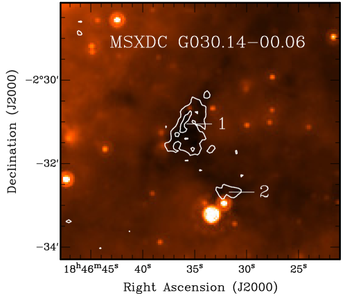
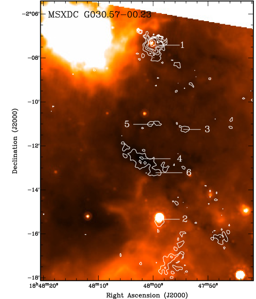
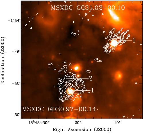
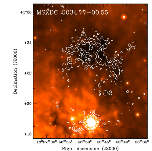
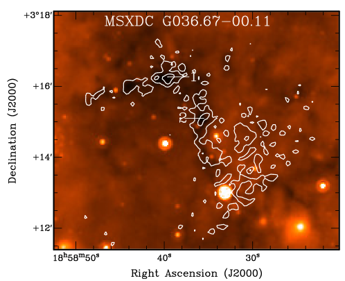
Figure A-20: Spitzer  24 $\mu$m  image overlaid with 1.2 mm continuum emission for G030.14$-$00.06  (contour levels are 30, 60 mJy beam^-1). The lower panels show the broadband SEDs for cores within this IRDC. The fluxes derived from the millimeter, sub-millimeter, and far-IR continuum data are shown as filled circles (with the corresponding error bars), while the 24 $\mu$m  fluxes are shown as either a filled circle (when included within the fit), an open circle (when excluded from the fit), or as an upper limit arrow. For cores that have measured fluxes only in the millimeter/sub-millimeter regime (i.e.  a limit at 24 $\mu$m), we show the results from two fits: one using only the measured fluxes (solid line; lower limit), while the other includes the 24 $\mu$m  limit as a real data (dashed line; upper limit). In all other cases, the solid line is the best fit gray-body, while the dotted lines correspond to the functions determined using the errors for the T_D, $\tau$, and $\beta$ output from the fitting. Labeled on each plot is the IRDC and core name, classification, and the derived parameters.

Figure A-21: Spitzer  24 $\mu$m  image overlaid with 1.2 mm continuum emission for G030.57$-$00.23  (contour levels are 30, 60, 90, 120, 240, 360, 480 mJy beam^-1). The lower panels show the broadband SEDs for the cores within this IRDC. The lower panels show the broadband SEDs for cores within this IRDC. The fluxes derived from the millimeter, sub-millimeter, and far-IR continuum data are shown as filled circles (with the corresponding error bars), while the 24 $\mu$m  fluxes are shown as either a filled circle (when included within the fit), an open circle (when excluded from the fit), or as an upper limit arrow. For cores that have measured fluxes only in the millimeter/sub-millimeter regime (i.e.  a limit at 24 $\mu$m), we show the results from two fits: one using only the measured fluxes (solid line; lower limit), while the other includes the 24 $\mu$m  limit as a real data (dashed line; upper limit). In all other cases, the solid line is the best fit gray-body, while the dotted lines correspond to the functions determined using the errors for the T_D, $\tau$, and $\beta$ output from the fitting. Labeled on each plot is the IRDC and core name, classification, and the derived parameters.

Figure A-22: Spitzer  24 $\mu$m  image overlaid with 1.2 mm continuum emission for G031.02$-$00.10  and G030.97$-$00.14  (contour levels are 40, 60, 80 mJy beam^-1). The lower panels show the broadband SEDs for cores within this IRDC. The fluxes derived from the millimeter, sub-millimeter, and far-IR continuum data are shown as filled circles (with the corresponding error bars), while the 24 $\mu$m  fluxes are shown as either a filled circle (when included within the fit), an open circle (when excluded from the fit), or as an upper limit arrow. For cores that have measured fluxes only in the millimeter/sub-millimeter regime (i.e.  a limit at 24 $\mu$m), we show the results from two fits: one using only the measured fluxes (solid line; lower limit), while the other includes the 24 $\mu$m  limit as a real data (dashed line; upper limit). In all other cases, the solid line is the best fit gray-body, while the dotted lines correspond to the functions determined using the errors for the T_D, $\tau$, and $\beta$ output from the fitting. Labeled on each plot is the IRDC and core name, classification, and the derived parameters.

Figure A-23: Spitzer  24 $\mu$m  image overlaid with 1.2 mm continuum emission for G031.97+00.07  (contour levels are 30, 60, 90,120, 240, 360, 480 mJy beam^-1). The lower panels show the broadband SEDs for cores within this IRDC. The fluxes derived from the millimeter, sub-millimeter, and far-IR continuum data are shown as filled circles (with the corresponding error bars), while the 24 $\mu$m  fluxes are shown as either a filled circle (when included within the fit), an open circle (when excluded from the fit), or as an upper limit arrow. For cores that have measured fluxes only in the millimeter/sub-millimeter regime (i.e.  a limit at 24 $\mu$m), we show the results from two fits: one using only the measured fluxes (solid line; lower limit), while the other includes the 24 $\mu$m  limit as a real data (dashed line; upper limit). In all other cases, the solid line is the best fit gray-body, while the dotted lines correspond to the functions determined using the errors for the T_D, $\tau$, and $\beta$ output from the fitting. Labeled on each plot is the IRDC and core name, classification, and the derived parameters.

Figure A-24: Spitzer  24 $\mu$m  image overlaid with 1.2 mm continuum emission for G033.69$-$00.01  (contour levels are 30, 60, 90, 120, 240 mJy beam^-1). The lower panels show the broadband SEDs for cores within this IRDC. The fluxes derived from the millimeter, sub-millimeter, and far-IR continuum data are shown as filled circles (with the corresponding error bars), while the 24 $\mu$m  fluxes are shown as either a filled circle (when included within the fit), an open circle (when excluded from the fit), or as an upper limit arrow. For cores that have measured fluxes only in the millimeter/sub-millimeter regime (i.e.  a limit at 24 $\mu$m), we show the results from two fits: one using only the measured fluxes (solid line; lower limit), while the other includes the 24 $\mu$m  limit as a real data (dashed line; upper limit). In all other cases, the solid line is the best fit gray-body, while the dotted lines correspond to the functions determined using the errors for the T_D, $\tau$, and $\beta$ output from the fitting. Labeled on each plot is the IRDC and core name, classification, and the derived parameters.

Figure A-25: Spitzer  24 $\mu$m  image overlaid with 1.2 mm continuum emission for G034.43+00.24  (contour levels are 60, 90, 120, 240, 360, 480, 840, 1200 mJy beam^-1). The lower panels show the broadband SEDs for cores within this IRDC. The fluxes derived from the millimeter, sub-millimeter, and far-IR continuum data are shown as filled circles (with the corresponding error bars), while the 24 $\mu$m  fluxes are shown as either a filled circle (when included within the fit), an open circle (when excluded from the fit), or as an upper limit arrow. For cores that have measured fluxes only in the millimeter/sub-millimeter regime (i.e.  a limit at 24 $\mu$m), we show the results from two fits: one using only the measured fluxes (solid line; lower limit), while the other includes the 24 $\mu$m  limit as a real data (dashed line; upper limit). In all other cases, the solid line is the best fit gray-body, while the dotted lines correspond to the functions determined using the errors for the T_D, $\tau$, and $\beta$ output from the fitting. Labeled on each plot is the IRDC and core name, classification, and the derived parameters.

Figure A-26: Spitzer  24 $\mu$m  image overlaid with 1.2 mm continuum emission for G034.77$-$00.55  (contour levels are 30, 60, 90, 120, 240 mJy beam^-1). The lower panels show the broadband SEDs for cores within this IRDC. The fluxes derived from the millimeter, sub-millimeter, and far-IR continuum data are shown as filled circles (with the corresponding error bars), while the 24 $\mu$m  fluxes are shown as either a filled circle (when included within the fit), an open circle (when excluded from the fit), or as an upper limit arrow. For cores that have measured fluxes only in the millimeter/sub-millimeter regime (i.e.  a limit at 24 $\mu$m), we show the results from two fits: one using only the measured fluxes (solid line; lower limit), while the other includes the 24 $\mu$m  limit as a real data (dashed line; upper limit). In all other cases, the solid line is the best fit gray-body, while the dotted lines correspond to the functions determined using the errors for the T_D, $\tau$, and $\beta$ output from the fitting. Labeled on each plot is the IRDC and core name, classification, and the derived parameters.

Figure A-27: Spitzer  24 $\mu$m  image overlaid with 1.2 mm continuum emission for G035.59-00.24  and G035.39$-$00.33  (contour levels are 30, 60, 90, 120 mJy beam^-1). The lower panels show the broadband SEDs for cores within this IRDC. The fluxes derived from the millimeter, sub-millimeter, and far-IR continuum data are shown as filled circles (with the corresponding error bars), while the 24 $\mu$m  fluxes are shown as either a filled circle (when included within the fit), an open circle (when excluded from the fit), or as an upper limit arrow. For cores that have measured fluxes only in the millimeter/sub-millimeter regime (i.e.  a limit at 24 $\mu$m), we show the results from two fits: one using only the measured fluxes (solid line; lower limit), while the other includes the 24 $\mu$m  limit as a real data (dashed line; upper limit). In all other cases, the solid line is the best fit gray-body, while the dotted lines correspond to the functions determined using the errors for the T_D, $\tau$, and $\beta$ output from the fitting. Labeled on each plot is the IRDC and core name, classification, and the derived parameters.

Figure A-28: Spitzer  24 $\mu$m  image overlaid with 1.2 mm continuum emission for G036.67$-$00.11  (contour levels are 30, 60, 90, 120 mJy beam^-1). The lower panels show the broadband SEDs for cores within this IRDC. The fluxes derived from the millimeter, sub-millimeter, and far-IR continuum data are shown as filled circles (with the corresponding error bars), while the 24 $\mu$m  fluxes are shown as either a filled circle (when included within the fit), an open circle (when excluded from the fit), or as an upper limit arrow. For cores that have measured fluxes only in the millimeter/sub-millimeter regime (i.e.  a limit at 24 $\mu$m), we show the results from two fits: one using only the measured fluxes (solid line; lower limit), while the other includes the 24 $\mu$m  limit as a real data (dashed line; upper limit). In all other cases, the solid line is the best fit gray-body, while the dotted lines correspond to the functions determined using the errors for the T_D, $\tau$, and $\beta$ output from the fitting. Labeled on each plot is the IRDC and core name, classification, and the derived parameters.

Figure A-29: Spitzer  24 $\mu$m  image overlaid with 1.2 mm continuum emission for G038.95$-$0.47  (contour levels are 30, 60, 90, 120 mJy beam^-1). The lower panels show the broadband SEDs for cores within this IRDC. The fluxes derived from the millimeter, sub-millimeter, and far-IR continuum data are shown as filled circles (with the corresponding error bars), while the 24 $\mu$m  fluxes are shown as either a filled circle (when included within the fit), an open circle (when excluded from the fit), or as an upper limit arrow. For cores that have measured fluxes only in the millimeter/sub-millimeter regime (i.e.  a limit at 24 $\mu$m), we show the results from two fits: one using only the measured fluxes (solid line; lower limit), while the other includes the 24 $\mu$m  limit as a real data (dashed line; upper limit). In all other cases, the solid line is the best fit gray-body, while the dotted lines correspond to the functions determined using the errors for the T_D, $\tau$, and $\beta$ output from the fitting. Labeled on each plot is the IRDC and core name, classification, and the derived parameters.

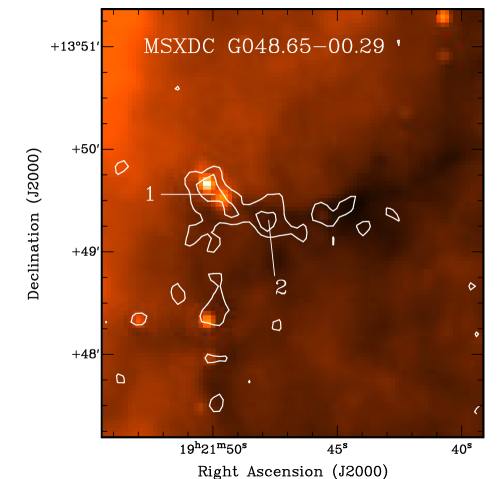
Figure A-30: Spitzer  24 $\mu$m  image overlaid with 1.2 mm continuum emission for G048.65$-$00.29  (contour levels are 30, 60, 90 mJy beam^-1). The lower panels show the broadband SEDs for cores within this IRDC. The fluxes derived from the millimeter, sub-millimeter, and far-IR continuum data are shown as filled circles (with the corresponding error bars), while the 24 $\mu$m  fluxes are shown as either a filled circle (when included within the fit), an open circle (when excluded from the fit), or as an upper limit arrow. For cores that have measured fluxes only in the millimeter/sub-millimeter regime (i.e.  a limit at 24 $\mu$m), we show the results from two fits: one using only the measured fluxes (solid line; lower limit), while the other includes the 24 $\mu$m  limit as a real data (dashed line; upper limit). In all other cases, the solid line is the best fit gray-body, while the dotted lines correspond to the functions determined using the errors for the T_D, $\tau$, and $\beta$ output from the fitting. Labeled on each plot is the IRDC and core name, classification, and the derived parameters.

Figure A-31: Spitzer  24 $\mu$m  image overlaid with 1.2 mm continuum emission for G053.11+00.05  (contour levels are 30, 60, 90, 120, 240, 360, 480 mJy beam^-1). The lower panels show the broadband SEDs for cores within this IRDC. The fluxes derived from the millimeter, sub-millimeter, and far-IR continuum data are shown as filled circles (with the corresponding error bars), while the 24 $\mu$m  fluxes are shown as either a filled circle (when included within the fit), an open circle (when excluded from the fit), or as an upper limit arrow. For cores that have measured fluxes only in the millimeter/sub-millimeter regime (i.e.  a limit at 24 $\mu$m), we show the results from two fits: one using only the measured fluxes (solid line; lower limit), while the other includes the 24 $\mu$m  limit as a real data (dashed line; upper limit). In all other cases, the solid line is the best fit gray-body, while the dotted lines correspond to the functions determined using the errors for the T_D, $\tau$, and $\beta$ output from the fitting. Labeled on each plot is the IRDC and core name, classification, and the derived parameters.

Figure A-32: Spitzer  24 $\mu$m  image overlaid with 1.2 mm continuum emission for G053.31+00.00  and G053.25+00.04  (contour levels are 30, 60, 90, 120, 240 mJy beam^-1). The lower panels show the broadband SEDs for cores within this IRDC. The fluxes derived from the millimeter, sub-millimeter, and far-IR continuum data are shown as filled circles (with the corresponding error bars), while the 24 $\mu$m  fluxes are shown as either a filled circle (when included within the fit), an open circle (when excluded from the fit), or as an upper limit arrow. For cores that have measured fluxes only in the millimeter/sub-millimeter regime (i.e.  a limit at 24 $\mu$m), we show the results from two fits: one using only the measured fluxes (solid line; lower limit), while the other includes the 24 $\mu$m  limit as a real data (dashed line; upper limit). In all other cases, the solid line is the best fit gray-body, while the dotted lines correspond to the functions determined using the errors for the T_D, $\tau$, and $\beta$ output from the fitting. Labeled on each plot is the IRDC and core name, classification, and the derived parameters.

Table A-1: Core coordinates, distances, and measured fluxes

IRDC core	Coordinates		D	F24	F55	F65	F75	F85	F95	F350	F450	F850	F1.2
	(J2000)	(J2000)	(kpc)	(Jy)	(Jy)	(Jy)	(Jy)	(Jy)	(Jy)	(Jy)	(Jy)	(Jy)	(Jy)
G015.05+00.07 MM1	18:17:50.4	$-$15:53:38	3.1	$<$ 0.05	…	…	…	…	…	3.92	3.96	…	0.12
G015.05+00.07 MM2	18:17:40.0	$-$15:48:55	3.1	$<$ 0.05	…	…	…	…	…	0.29	…	…	0.05
G015.05+00.07 MM3	18:17:42.4	$-$15:47:03	3.1	$<$ 0.06	…	…	…	…	…	…	…	…	0.04
G015.05+00.07 MM4	18:17:32.0	$-$15:46:35	3.1	$<$ 0.07	…	…	…	…	…	0.78	…	…	0.04
G015.05+00.07 MM5	18:17:40.2	$-$15:49:47	3.1	$<$ 0.06	…	…	…	…	…	0.56	…	…	0.03
G015.31$-$00.16 MM1	18:18:56.4	$-$15:45:00	1.9	0.19	4.83	5.72	9.62	14.11	17.00	1.64	…	…	0.04
G015.31$-$00.16 MM2	18:18:50.4	$-$15:43:19	1.9	0.02	0.52	0.75	3.09	3.86	8.91	0.80	…	…	0.04
G015.31$-$00.16 MM3	18:18:45.3	$-$15:41:58	1.9	$<$ 0.06	…	…	…	…	…	…	…	…	0.04
G015.31$-$00.16 MM4	18:18:48.0	$-$15:44:22	1.9	$<$ 0.06	…	…	…	…	…	0.52	…	…	0.02
G015.31$-$00.16 MM5	18:18:49.1	$-$15:42:47	1.9	$<$ 0.06	…	…	…	…	…	0.88	…	…	0.02
G018.82$-$00.28 MM1	18:25:56.1	$-$12:42:48	4.6	0.09	37.24	75.26	121.74	170.28	196.23	41.19	24.01	…	0.46
G018.82$-$00.28 MM2	18:26:23.4	$-$12:39:37	4.6	1.12	247.76	278.54	296.29	307.25	271.01	19.12	9.54	…	0.17
G018.82$-$00.28 MM3	18:25:52.6	$-$12:44:37	4.6	0.19	…	…	…	…	…	14.74	9.02	…	0.12
G018.82$-$00.28 MM4	18:26:15.5	$-$12:41:32	4.6	0.01	0.05	0.89	2.63	3.26	9.81	3.38	…	…	0.08
G018.82$-$00.28 MM5	18:26:21.0	$-$12:41:11	4.6	$<$ 0.06	…	…	…	…	…	1.79	0.78	…	0.06
G018.82$-$00.28 MM6	18:26:18.4	$-$12:41:15	4.6	$<$ 0.06	…	…	…	…	…	…	…	…	0.05
G019.27+00.07 MM1	18:25:58.5	$-$12:03:59	2.4	0.16	…	…	…	…	…	20.28	4.89	0.85	0.15
G019.27+00.07 MM2	18:25:52.6	$-$12:04:48	2.4	0.03	…	…	…	…	…	8.36	3.13	0.62	0.09
G022.35+00.41 MM1	18:30:24.4	$-$09:10:34	3.7	0.02	0.99	0.71	2.29	3.65	4.63	13.47	5.07	1.54	0.35
G022.35+00.41 MM2	18:30:24.2	$-$09:12:44	3.7	0.08	8.16	11.96	11.90	15.51	14.10	1.25	…	…	0.07
G022.35+00.41 MM3	18:30:38.1	$-$09:12:44	3.7	$<$ 0.06	…	…	…	…	…	…	…	0.16	0.05
G022.73+00.11 MM1	18:32:13.0	$-$09:00:50	4.9	$<$ 0.05	…	1.18	1.77	2.59	7.82	0.60	…	…	0.04
G023.60+00.00 MM1	18:34:11.6	$-$08:19:06	3.7	0.19	10.95	23.12	33.82	40.28	41.22	25.12	17.00	…	0.38
G023.60+00.00 MM2	18:34:21.1	$-$08:18:07	3.7	1.25	43.63	68.07	80.64	105.90	111.44	19.38	12.04	…	0.27
G023.60+00.00 MM3	18:34:10.0	$-$08:18:28	3.7	$<$ 0.11	15.64	17.30	21.92	31.98	31.66	1.38	0.98	…	0.08
G023.60+00.00 MM4	18:34:23.0	$-$08:18:21	3.7	$<$ 0.18	…	…	…	…	…	2.44	1.64	…	0.07
G023.60+00.00 MM5	18:34:09.5	$-$08:18:00	3.7	1.54	…	…	…	…	…	2.56	1.60	…	0.07
G023.60+00.00 MM6	18:34:18.2	$-$08:18:52	3.7	$<$ 0.09	…	…	…	…	…	…	0.42	…	0.06
G023.60+00.00 MM7	18:34:21.1	$-$08:17:11	3.7	0.22	3.76	5.99	6.44	7.88	8.07	0.73	0.54	…	0.06
G023.60+00.00 MM8	18:34:24.9	$-$08:17:14	3.7	$<$ 0.12	…	…	…	…	…	0.66	…	…	0.04
G023.60+00.00 MM9	18:34:22.5	$-$08:16:04	3.7	$<$ 0.08	…	…	…	…	…	0.62	0.33	…	0.04
G024.08+00.04 MM1	18:34:57.0	$-$07:43:26	3.7	0.77	…	…	…	…	…	31.16	11.18	…	0.22
G024.08+00.04 MM2	18:34:51.1	$-$07:45:32	3.7	$<$ 0.10	7.22	9.36	15.33	22.90	23.23	3.36	1.24	…	0.07
G024.08+00.04 MM3	18:35:02.2	$-$07:45:25	3.7	$<$ 0.06	…	…	…	…	…	2.12	1.04	…	0.05
G024.08+00.04 MM4	18:35:02.6	$-$07:45:56	3.7	$<$ 0.06	0.88	1.69	2.88	2.53	5.16	1.31	0.54	…	0.05
G024.08+00.04 MM5	18:35:07.4	$-$07:45:46	3.7	$<$ 0.06	…	…	…	…	…	1.50	0.80	…	0.04
G024.33+00.11 MM1	18:35:07.9	$-$07:35:04	6.3	0.85	…	…	…	…	…	64.99	52.41	…	1.20
G024.33+00.11 MM10	18:35:27.9	$-$07:35:32	3.7	0.02	…	…	…	…	…	1.64	…	…	0.06
G024.33+00.11 MM11	18:35:05.1	$-$07:35:58	3.7	$<$ 0.07	…	…	…	…	…	1.09	1.15	…	0.05
G024.33+00.11 MM2	18:35:34.5	$-$07:37:28	3.7	$<$ 0.10	…	…	…	…	…	2.13	…	…	0.12
G024.33+00.11 MM3	18:35:27.9	$-$07:36:18	3.7	$<$ 0.10	…	…	…	…	…	3.11	…	…	0.10
G024.33+00.11 MM4	18:35:19.4	$-$07:37:17	3.7	$<$ 0.08	…	…	…	…	…	2.04	…	…	0.09
G024.33+00.11 MM5	18:35:33.8	$-$07:36:42	3.7	$<$ 0.13	…	…	…	…	…	1.74	…	…	0.08
G024.33+00.11 MM6	18:35:07.7	$-$07:34:33	3.7	$<$ 0.08	…	…	…	…	…	2.45	…	…	0.08
G024.33+00.11 MM7	18:35:09.8	$-$07:39:48	3.7	$<$ 0.07	…	…	…	…	…	…	…	…	0.08
G024.33+00.11 MM8	18:35:23.4	$-$07:37:21	3.7	$<$ 0.09	…	…	…	…	…	1.31	…	…	0.07
G024.33+00.11 MM9	18:35:26.5	$-$07:36:56	3.7	1.16	…	…	…	…	…	1.92	…	…	0.07
G024.60+00.08 MM1	18:35:41.1	$-$07:18:30	3.6	0.35	13.69	24.03	37.79	52.35	69.80	26.73	7.03	1.37	0.26
G024.60+00.08 MM2	18:35:39.3	$-$07:18:51	6.5	0.02	6.96	19.99	38.49	56.80	72.71	28.38	8.46	1.30	0.26
G024.60+00.08 MM3	18:35:40.2	$-$07:18:37	3.6	$<$ 0.09	…	…	…	…	…	5.04	…	…	0.26
G024.60+00.08 MM4	18:35:35.7	$-$07:18:09	3.6	$<$ 0.07	…	…	…	…	…	…	…	…	0.23
G025.04$-$00.20 MM1	18:38:10.2	$-$07:02:34	4.1	0.17	9.55	13.33	18.24	22.96	23.19	5.96	2.80	…	0.20
G025.04$-$00.20 MM2	18:38:17.7	$-$07:02:51	4.1	0.01	0.52	0.62	0.89	0.90	1.70	…	2.17	…	0.09
G025.04$-$00.20 MM3	18:38:10.2	$-$07:02:44	4.1	$<$ 0.07	…	…	…	…	…	2.01	2.50	…	0.09
G025.04$-$00.20 MM4	18:38:13.7	$-$07:03:12	4.1	$<$ 0.06	…	…	…	…	…	…	1.20	…	0.08
G025.04$-$00.20 MM5	18:38:12.0	$-$07:02:44	4.1	$<$ 0.06	…	…	…	…	…	0.86	1.33	…	0.07
G027.75+00.16 MM1	18:41:19.9	$-$04:32:20	4.8	0.05	0.67	1.31	3.40	5.86	9.72	3.16	…	…	0.08
G027.75+00.16 MM2	18:41:33.0	$-$04:33:44	4.8	$<$ 0.06	2.57	4.85	9.15	12.72	16.93	…	…	…	0.05
G027.75+00.16 MM3	18:41:16.8	$-$04:31:55	4.8	0.01	…	…	…	…	…	0.68	…	…	0.04
G027.75+00.16 MM4	18:41:30.4	$-$04:30:00	4.8	$<$ 0.05	…	…	…	…	…	1.82	…	…	0.03
G027.75+00.16 MM5	18:41:23.6	$-$04:30:42	4.8	$<$ 0.05	…	0.52	1.68	2.81	6.64	1.07	…	…	0.03
G027.94$-$00.47 MM1	18:44:03.6	$-$04:38:00	3.2	1.10	…	…	…	…	…	4.41	2.41	…	0.10
G027.94$-$00.47 MM2	18:44:03.1	$-$04:37:25	3.2	$<$ 0.06	…	…	…	…	…	0.20	…	…	0.04
G027.97$-$00.42 MM1	18:43:52.8	$-$04:36:13	3.2	0.05	…	…	…	…	…	6.33	5.91	…	0.14
G027.97$-$00.42 MM2	18:43:58.0	$-$04:34:24	3.2	0.22	…	…	…	…	…	9.06	5.44	…	0.10
G027.97$-$00.42 MM3	18:43:54.9	$-$04:36:08	3.2	$<$ 0.05	…	…	…	…	…	…	…	…	0.04
G028.04$-$00.46 MM1	18:44:08.5	$-$04:33:22	3.2	0.32	…	…	…	…	…	4.42	3.69	…	0.09
G028.08+00.07 MM1	18:42:20.3	$-$04:16:42	4.7	$<$ 0.05	…	…	0.50	1.18	4.61	1.03	0.68	…	0.06
G028.10$-$00.45 MM1	18:44:12.9	$-$04:29:45	3.2	$<$ 0.05	…	…	…	…	…	0.25	…	…	0.03
G028.10$-$00.45 MM2	18:44:14.3	$-$04:29:48	3.2	$<$ 0.05	…	…	…	…	…	0.45	…	…	0.02
G028.23$-$00.19 MM1	18:43:30.7	$-$04:13:12	4.8	$<$ 0.04	…	…	…	4.69	1.48	1.67	0.97	…	0.08
G028.23$-$00.19 MM2	18:43:29.0	$-$04:12:16	4.8	$<$ 0.06	…	…	…	…	…	1.01	0.30	…	0.04
G028.23$-$00.19 MM3	18:43:30.0	$-$04:12:33	4.8	$<$ 0.05	…	…	…	…	…	…	0.20	…	0.02
G028.28$-$00.34 MM1	18:44:15.0	$-$04:17:54	3.2	2.00	…	…	…	…	…	15.66	11.06	…	0.32
G028.28$-$00.34 MM2	18:44:21.3	$-$04:17:37	3.2	2.00	…	…	…	…	…	12.00	5.54	…	0.17
G028.28$-$00.34 MM3	18:44:13.4	$-$04:18:05	3.2	1.50	…	…	…	…	…	7.67	7.55	…	0.14
G028.28$-$00.34 MM4	18:44:11.4	$-$04:17:22	3.2	$<$ 0.18	…	…	…	…	…	…	…	…	0.06
G028.37+00.07 MM1	18:42:52.1	$-$03:59:45	4.8	0.12	…	…	…	…	…	75.35	37.33	…	0.47
G028.37+00.07 MM10	18:42:54.0	$-$04:02:30	4.8	0.02	…	…	…	…	…	4.13	2.59	…	0.09
G028.37+00.07 MM11	18:42:42.7	$-$04:01:44	4.8	0.01	…	…	…	…	…	1.94	1.21	…	0.08
G028.37+00.07 MM12	18:43:09.9	$-$04:06:52	4.8	$<$ 0.07	…	…	…	…	…	…	…	…	0.07
G028.37+00.07 MM13	18:42:41.8	$-$03:57:08	4.8	0.31	…	…	…	…	…	…	…	…	0.07
G028.37+00.07 MM14	18:42:52.6	$-$04:02:44	4.8	$<$ 0.04	…	…	…	…	…	0.85	1.00	…	0.06
G028.37+00.07 MM15	18:42:32.4	$-$04:01:16	4.8	0.28	…	…	…	…	…	…	…	…	0.06
G028.37+00.07 MM16	18:42:40.2	$-$04:00:23	4.8	$<$ 0.05	…	…	…	…	…	1.81	1.37	…	0.06
G028.37+00.07 MM17	18:43:00.0	$-$04:01:34	4.8	$<$ 0.04	…	…	…	…	…	0.72	0.36	…	0.06
G028.37+00.07 MM18	18:43:12.9	$-$04:01:16	4.8	0.43	…	…	…	…	…	…	…	…	0.05
G028.37+00.07 MM2	18:42:37.6	$-$04:02:05	4.8	1.74	…	…	…	…	…	26.54	12.66	…	0.28
G028.37+00.07 MM3	18:43:03.1	$-$04:06:24	4.8	0.15	…	…	…	…	…	…	…	…	0.25
G028.37+00.07 MM4	18:42:50.7	$-$04:03:15	4.8	0.04	…	…	…	…	…	7.96	6.48	…	0.20
G028.37+00.07 MM5	18:42:26.8	$-$04:01:30	4.8	$<$ 0.00	…	…	…	…	…	…	…	…	0.15
G028.37+00.07 MM6	18:42:49.0	$-$04:02:23	4.8	$<$ 0.04	…	…	…	…	…	5.22	3.75	…	0.15
G028.37+00.07 MM7	18:42:56.3	$-$04:07:31	4.8	0.21	…	…	…	…	…	…	…	…	0.14
G028.37+00.07 MM8	18:42:49.7	$-$04:09:54	4.8	1.05	…	…	…	…	…	…	…	…	0.12
G028.37+00.07 MM9	18:42:46.7	$-$04:04:08	4.8	$<$ 0.04	…	…	…	…	…	2.24	2.05	…	0.10
G028.53$-$00.25 MM1	18:44:18.0	$-$03:59:34	5.2	$<$ 0.05	…	…	…	2.03	3.88	5.25	4.90	1.05	0.23
G028.53$-$00.25 MM10	18:44:18.5	$-$03:58:43	5.2	$<$ 0.05	…	…	…	…	…	…	0.64	…	0.06
G028.53$-$00.25 MM2	18:44:15.7	$-$03:59:41	5.2	0.02	…	…	…	…	…	2.37	2.07	0.48	0.13
G028.53$-$00.25 MM3	18:44:16.0	$-$04:00:48	5.2	$<$ 0.05	…	0.84	1.65	4.70	11.03	2.30	1.55	0.38	0.13
G028.53$-$00.25 MM4	18:44:18.6	$-$04:00:05	5.2	0.02	…	…	…	…	…	1.50	0.82	…	0.10
G028.53$-$00.25 MM5	18:44:17.0	$-$04:02:04	5.2	0.01	…	…	…	…	…	…	2.28	0.57	0.10
G028.53$-$00.25 MM6	18:44:17.8	$-$04:00:05	5.2	$<$ 0.05	…	…	…	…	…	0.85	0.87	…	0.07
G028.53$-$00.25 MM7	18:44:23.7	$-$04:02:09	5.2	$<$ 0.05	…	…	0.76	1.08	1.51	…	0.80	0.13	0.06
G028.53$-$00.25 MM8	18:44:22.0	$-$04:01:35	5.2	$<$ 0.05	…	…	…	…	…	0.47	…	0.20	0.06
G028.53$-$00.25 MM9	18:44:19.3	$-$03:58:05	5.2	$<$ 0.05	…	…	…	…	…	0.83	…	0.29	0.06
G028.67+00.13 MM1	18:43:03.1	$-$03:41:41	4.8	2.51	…	…	…	…	…	8.66	4.27	…	0.09
G028.67+00.13 MM2	18:43:07.1	$-$03:44:01	4.8	0.04	0.64	1.19	2.63	4.37	7.63	1.60	1.37	…	0.07
G028.67+00.13 MM3	18:42:58.2	$-$03:48:20	4.8	0.36	…	…	…	…	…	…	…	…	0.06
G028.67+00.13 MM4	18:43:13.2	$-$03:41:03	4.8	0.01	…	…	…	…	…	…	…	…	0.04
G028.67+00.13 MM5	18:43:10.1	$-$03:45:08	4.8	$<$ 0.05	…	…	…	…	…	0.90	0.39	…	0.03
G028.67+00.13 MM6	18:43:12.2	$-$03:45:39	4.8	$<$ 0.06	…	…	…	…	…	0.71	0.33	…	0.03
G028.67+00.13 MM7	18:43:06.9	$-$03:45:11	4.8	$<$ 0.05	…	…	…	…	…	…	…	…	0.03
G030.14$-$00.06 MM1	18:46:35.7	$-$02:31:03	5.2	$<$ 0.07	1.07	1.62	4.07	6.89	16.87	0.95	0.77	…	0.05
G030.14$-$00.06 MM2	18:46:31.7	$-$02:32:41	5.2	$<$ 0.01	…	…	…	…	…	1.07	0.52	…	0.04
G030.57$-$00.23 MM1	18:48:00.0	$-$02:07:20	5.2	0.57	…	…	…	…	…	…	…	…	0.30
G030.57$-$00.23 MM2	18:47:58.7	$-$02:15:20	5.2	1.31	…	…	…	…	…	…	…	…	0.14
G030.57$-$00.23 MM3	18:47:54.5	$-$02:11:15	5.2	0.01	2.41	2.91	5.79	10.67	15.24	…	…	…	0.06
G030.57$-$00.23 MM4	18:48:01.8	$-$02:12:35	5.2	$<$ 0.06	1.38	2.27	5.17	5.15	4.57	1.25	…	…	0.04
G030.57$-$00.23 MM5	18:47:59.9	$-$02:11:01	5.2	$<$ 0.08	…	…	…	…	…	…	…	…	0.04
G030.57$-$00.23 MM6	18:47:59.4	$-$02:13:13	5.2	0.01	…	…	…	…	…	…	…	…	0.03
G030.97$-$00.14 MM1	18:48:21.6	$-$01:48:27	4.8	1.66	106.60	127.42	136.46	130.72	122.59	16.44	11.21	1.23	0.11
G030.97$-$00.14 MM2	18:48:22.0	$-$01:47:42	4.8	$<$ 0.07	…	…	…	…	…	…	…	…	0.03
G031.02$-$00.10 MM1	18:48:09.9	$-$01:45:17	4.8	$<$ 0.08	…	…	…	…	…	…	…	…	0.13
G031.97+00.07 MM1	18:49:36.3	00:45:45	6.1	0.86	…	…	…	…	…	48.79	40.60	5.49	0.91
G031.97+00.07 MM2	18:49:36.0	00:46:16	6.1	$<$ 0.07	…	…	…	…	…	9.78	10.68	1.08	0.31
G031.97+00.07 MM3	18:49:32.3	00:47:02	6.1	$<$ 0.07	…	…	…	…	…	5.67	4.70	0.75	0.19
G031.97+00.07 MM4	18:49:33.0	00:47:33	6.1	0.02	…	…	…	…	…	2.18	2.45	0.41	0.12
G031.97+00.07 MM5	18:49:21.9	00:50:35	6.1	0.01	…	…	…	…	…	1.89	2.35	0.47	0.10
G031.97+00.07 MM6	18:49:35.0	00:46:44	6.1	$<$ 0.08	…	…	…	…	…	2.97	2.57	0.66	0.10
G031.97+00.07 MM7	18:49:28.4	00:48:54	6.1	$<$ 0.04	…	…	…	…	…	0.87	1.08	0.45	0.08
G031.97+00.07 MM8	18:49:29.1	00:48:12	6.1	0.21	…	…	…	…	…	1.44	1.07	…	0.06
G031.97+00.07 MM9	18:49:31.6	00:46:30	6.1	$<$ 0.07	…	…	…	…	…	…	…	…	0.05
G033.69$-$00.01 MM1	18:52:58.8	00:42:37	7.1	0.21	7.25	12.68	19.62	25.87	36.12	14.61	13.32	…	0.21
G033.69$-$00.01 MM10	18:52:52.7	00:38:35	7.1	$<$ 0.05	…	…	…	…	…	1.10	1.22	…	0.04
G033.69$-$00.01 MM11	18:52:56.2	00:41:48	7.1	$<$ 0.05	…	…	…	…	…	1.10	1.17	…	0.03
G033.69$-$00.01 MM2	18:52:49.9	00:37:57	7.1	2.54	…	…	…	…	…	8.67	6.15	…	0.12
G033.69$-$00.01 MM3	18:52:50.8	00:36:43	7.1	0.76	…	…	…	…	…	3.36	2.85	…	0.08
G033.69$-$00.01 MM4	18:52:56.4	00:43:08	7.1	0.04	1.06	1.45	2.38	2.64	4.67	3.70	3.68	…	0.08
G033.69$-$00.01 MM5	18:52:47.8	00:36:47	7.1	0.97	…	…	…	…	…	6.07	4.52	…	0.06
G033.69$-$00.01 MM6	18:52:48.7	00:35:58	7.1	$<$ 0.05	…	…	…	…	…	1.20	…	…	0.05
G033.69$-$00.01 MM7	18:52:58.1	00:44:08	7.1	$<$ 0.05	…	…	…	…	…	…	…	…	0.04
G033.69$-$00.01 MM8	18:52:53.9	00:41:16	7.1	$<$ 0.05	…	…	…	…	…	1.36	1.04	…	0.04
G033.69$-$00.01 MM9	18:52:58.1	00:41:20	7.1	0.57	…	…	…	…	…	2.70	2.08	…	0.04
G034.43+00.24 MM1	18:53:18.0	01:25:24	3.7	1.46	…	…	…	…	…	147.14	50.85	10.10	2.23
G034.43+00.24 MM2	18:53:18.6	01:24:40	3.7	1.62	…	…	…	…	…	55.09	24.98	5.51	0.96
G034.43+00.24 MM3	18:53:20.4	01:28:23	3.7	0.12	18.85	31.21	42.72	51.51	55.65	12.36	9.63	1.57	0.24
G034.43+00.24 MM4	18:53:19.0	01:24:08	3.7	0.13	21.93	44.68	75.76	100.36	113.95	5.77	4.15	0.84	0.22
G034.43+00.24 MM5	18:53:19.8	01:23:30	3.7	$<$ 0.05	0.86	3.33	6.27	11.58	16.85	3.13	1.41	0.25	0.12
G034.43+00.24 MM6	18:53:18.6	01:27:48	3.7	$<$ 0.04	…	…	…	…	…	0.51	0.56	0.15	0.06
G034.43+00.24 MM7	18:53:18.3	01:27:13	3.7	$<$ 0.05	…	…	…	…	…	1.52	0.59	0.20	0.06
G034.43+00.24 MM8	18:53:16.4	01:26:20	3.7	$<$ 0.05	4.23	3.72	2.34	9.55	21.63	0.99	1.28	0.16	0.05
G034.43+00.24 MM9	18:53:18.4	01:28:14	3.7	$<$ 0.04	…	…	…	…	…	…	…	…	0.05
G034.77$-$00.55 MM1	18:56:48.2	01:18:47	2.9	2.04	…	…	…	…	…	…	…	…	0.23
G034.77$-$00.55 MM2	18:56:50.3	01:23:16	2.9	$<$ 0.04	1.79	1.64	2.62	3.19	6.30	…	…	…	0.06
G034.77$-$00.55 MM3	18:56:44.7	01:20:42	2.9	0.00	…	…	…	…	…	…	…	…	0.04
G034.77$-$00.55 MM4	18:56:48.9	01:23:34	2.9	$<$ 0.04	…	…	…	…	…	…	…	…	0.04
G035.39$-$00.33 MM1	18:56:41.2	02:09:52	3.0	$<$ 0.00	…	…	…	…	…	…	…	…	0.13
G035.39$-$00.33 MM2	18:56:59.2	02:04:53	3.0	0.27	…	…	…	…	…	…	…	…	0.11
G035.39$-$00.33 MM3	18:57:05.3	02:06:29	3.0	2.37	…	…	…	…	…	11.45	6.72	…	0.11
G035.39$-$00.33 MM4	18:57:06.7	02:08:23	3.0	0.01	…	…	…	…	…	1.80	1.08	…	0.08
G035.39$-$00.33 MM5	18:57:08.8	02:08:09	3.0	$<$ 0.04	0.15	0.81	0.69	2.16	4.29	…	…	…	0.07
G035.39$-$00.33 MM6	18:57:08.4	02:09:09	3.0	0.03	…	…	…	…	…	2.56	1.57	…	0.06
G035.39$-$00.33 MM7	18:57:08.1	02:10:50	3.0	0.02	…	…	…	…	…	2.18	1.48	…	0.06
G035.39$-$00.33 MM8	18:57:07.0	02:08:54	3.0	$<$ 0.04	…	…	…	…	…	0.33	…	…	0.05
G035.39$-$00.33 MM9	18:57:11.2	02:07:27	3.0	$<$ 0.03	…	…	…	…	…	…	0.86	…	0.05
G035.59$-$00.24 MM1	18:57:02.3	02:17:04	3.0	0.36	…	…	…	…	…	6.11	…	…	0.07
G035.59$-$00.24 MM2	18:57:07.4	02:16:14	3.0	0.02	2.01	4.11	7.49	12.73	17.87	2.17	…	…	0.06
G035.59$-$00.24 MM3	18:57:11.6	02:16:08	3.0	$<$ 0.03	…	…	…	…	…	0.65	…	…	0.04
G036.67$-$00.11 MM1	18:58:39.6	03:16:16	3.6	$<$ 0.03	0.11	0.90	1.59	4.05	5.14	1.52	…	…	0.06
G036.67$-$00.11 MM2	18:58:35.6	03:15:06	3.6	$<$ 0.03	0.29	0.39	1.71	4.21	9.51	…	…	…	0.05
G038.95$-$00.47 MM1	19:04:07.4	05:08:48	2.8	$<$ 0.03	0.02	0.49	0.55	0.80	3.84	4.04	2.81	0.79	0.12
G038.95$-$00.47 MM2	19:04:03.4	05:07:56	2.8	1.25	…	…	…	…	…	6.97	3.53	0.43	0.10
G038.95$-$00.47 MM3	19:04:07.4	05:09:44	2.8	0.00	…	…	…	…	…	3.31	1.94	0.33	0.07
G038.95$-$00.47 MM4	19:04:00.6	05:09:06	2.8	0.26	…	…	…	…	…	1.81	1.24	0.27	0.05
G048.65$-$00.29 MM1	19:21:49.7	13:49:30	2.6	0.10	…	…	…	…	…	4.02	2.39	…	0.07
G048.65$-$00.29 MM2	19:21:47.6	13:49:22	2.6	$<$ 0.04	…	…	…	…	…	1.19	1.34	…	0.06
G053.11+00.05 MM1	19:29:17.2	17:56:21	1.8	1.37	…	…	…	…	…	49.71	22.42	…	0.54
G053.11+00.05 MM2	19:29:20.2	17:57:06	1.8	0.18	…	…	…	…	…	4.78	2.45	…	0.08
G053.11+00.05 MM3	19:29:00.6	17:55:11	1.8	0.00	…	…	…	…	…	…	…	…	0.07
G053.11+00.05 MM4	19:29:20.4	17:55:04	1.8	0.23	…	…	…	…	…	2.76	1.09	…	0.05
G053.11+00.05 MM5	19:29:26.3	17:54:53	1.8	0.63	…	…	…	…	…	2.11	…	…	0.05
G053.25+00.04 MM1	19:29:39.0	18:01:42	2.0	0.06	…	…	…	…	…	8.15	4.30	…	0.25
G053.25+00.04 MM2	19:29:33.0	18:01:00	2.0	0.07	…	…	…	…	…	1.25	0.58	…	0.10
G053.25+00.04 MM3	19:29:44.0	17:58:47	2.0	0.01	…	…	…	…	…	2.70	0.93	…	0.10
G053.25+00.04 MM4	19:29:34.5	18:01:39	2.0	0.09	…	…	…	…	…	3.00	1.68	…	0.07
G053.25+00.04 MM5	19:29:39.4	17:58:40	2.0	0.01	…	…	…	…	…	1.79	0.65	…	0.05
G053.25+00.04 MM6	19:29:31.5	17:59:50	2.0	1.39	…	…	…	…	…	2.58	1.13	…	0.05
G053.31+00.00 MM1	19:29:50.0	18:05:07	2.0	$<$ 0.03	0.20	0.38	0.70	0.77	2.40	0.73	0.52	…	0.07
G053.31+00.00 MM2	19:29:42.1	18:03:57	2.0	$<$ 0.03	0.35	1.28	2.51	3.30	5.35	0.78	0.78	…	0.06
G053.31+00.00 MM3	19:29:49.7	18:04:39	2.0	0.00	0.95	1.63	2.51	3.28	5.18	1.58	0.79	…	0.02

Table A-2: Properties of the cores derived from gray-body fits to their broadband SEDs.

Table A-3: Properties of the cores for which limits where estimated from the gray-body fits to their broadband SEDs.

References

- Adams et al. (1987) Adams, F. C., Lada, C. J., & Shu, F. H. 1987, ApJ, 312, 788
- Andre & Montmerle (1994) Andre, P. & Montmerle, T. 1994, ApJ, 420, 837
- Beuther & Sridharan (2007) Beuther, H., & Sridharan, T. K. 2007, ApJ, 668, 348
- Beuther et al. (2005) Beuther, H., Sridharan, T. K., & Saito, M. 2005, ApJ, 634, L185
- Blitz (1991) Blitz, L. 1991, in NATO ASIC Proc. 342: The Physics of Star Formation and Early Stellar Evolution, 3–+
- Blitz & Williams (1999) Blitz, L. & Williams, J. P. 1999, in NATO ASIC Proc. 540: The Origin of Stars and Planetary Systems, 3–+
- Bok & Reilly (1947) Bok, B. J. & Reilly, E. F. 1947, ApJ, 105, 255
- Carey et al. (1998) Carey, S. J., Clark, F. O., Egan, M. P., Price, S. D., Shipman, R. F., & Kuchar, T. A. 1998, ApJ, 508, 721
- Carey et al. (2000) Carey, S. J., Feldman, P. A., Redman, R. O., Egan, M. P., MacLeod, J. M., & Price, S. D. 2000, ApJ, 543, L157
- Carey et al. (2005) Carey, S. J., Noriega-Crespo, A., Price, S. D., Padgett, D. L., Kraemer, K. E., Indebetouw, R., Mizuno, D. R., Ali, B., Berriman, G. B., Boulanger, F., Cutri, R. M., Ingalls, J. G., Kuchar, T. A., Latter, W. B., Marleau, F. R., Miville-Deschenes, M. A., Molinari, S., Rebull, L. M., & Testi, L. 2005, in Bulletin of the American Astronomical Society, Vol. 37, Bulletin of the American Astronomical Society, 1252–+
- Chambers et al. (2009) Chambers, E. T., Jackson, J. M., Rathborne, J. M., & Simon, R. 2009, ApJS, 181, 360
- Cyganowski et al. (2008) Cyganowski, C. J., et al. 2008, AJ, 136, 2391
- Egan et al. (1998) Egan, M. P., Shipman, R. F., Price, S. D., Carey, S. J., Clark, F. O., & Cohen, M. 1998, ApJ, 494, L199
- Garay et al. (2004) Garay, G., Faúndez, S., Mardones, D., Bronfman, L., Chini, R., & Nyman, L.-Å. 2004, ApJ, 610, 313
- Garay & Lizano (1999) Garay, G. & Lizano, S. 1999, PASP, 111, 1049
- Gordon (1995) Gordon, M. A. 1995, A&A, 301, 853
- Hennebelle et al. (2001) Hennebelle, P., Pérault, M., Teyssier, D., & Ganesh, S. 2001, A&A, 365, 598
- Hildebrand (1983) Hildebrand, R. H. 1983, QJRAS, 24, 267
- Iben (1965) Iben, I. J. 1965, ApJ, 141, 993
- Jackson et al. (2006) Jackson, J. M., Rathborne, J. M., Shah, R. Y., Simon, R., Bania, T. M., Clemens, D. P., Chambers, E. T., Johnson, A. M., Dormody, M., Lavoie, R., & Heyer, M. H. 2006, ApJS, 163, 145
- Krumholz & McKee (2008) Krumholz, M. R. & McKee, C. F. 2008, ArXiv e-prints, 801
- Lada & Lada (2003) Lada, C. J. & Lada, E. A. 2003, ARA&A, 41, 57
- Lada & Wilking (1984) Lada, C. J. & Wilking, B. A. 1984, ApJ, 287, 610
- Larson (2003) Larson, R. B. 2003, Galactic Star Formation Across the Stellar Mass Spectrum, 287, 65
- Lis & Carlstrom (1994) Lis, D. C. & Carlstrom, J. E. 1994, ApJ, 424, 189
- Marston et al. (2004) Marston, A. P., et al. 2004, ApJS, 154, 333
- Molinari et al. (2008) Molinari, S., Pezzuto, S., Cesaroni, R., Brand, J., Faustini, F., & Testi, L. 2008, A&A, 481, 345
- Myers & Benson (1983) Myers, P. C. & Benson, P. J. 1983, ApJ, 266, 309
- Noriega-Crespo et al. (2004) Noriega-Crespo, A., et al. 2004, ApJS, 154, 352
- Ormel et al. (2005) Ormel, C. W., Shipman, R. F., Ossenkopf, V., & Helmich, F. P. 2005, A&A, 439, 613
- Ossenkopf & Henning (1994) Ossenkopf, V. & Henning, T. 1994, A&A, 291, 943
- Palla & Stahler (1990) Palla, F. & Stahler, S. W. 1990, ApJ, 360, L47
- Perault et al. (1996) Perault, M., Omont, A., Simon, G., Seguin, P., Ojha, D., Blommaert, J., Felli, M., Gilmore, G., Guglielmo, F., Habing, H., Price, S., Robin, A., de Batz, B., Cesarsky, C., Elbaz, D., Epchtein, N., Fouque, P., Guest, S., Levine, D., Pollock, A., Prusti, T., Siebenmorgen, R., Testi, L., & Tiphene, D. 1996, A&A, 315, L165
- Pillai et al. (2006) Pillai, T., Wyrowski, F., Menten, K. M., & Krügel, E. 2006, A&A, 447, 929
- Rathborne et al. (2005) Rathborne, J. M., Jackson, J. M., Chambers, E. T., Simon, R., Shipman, R., & Frieswijk, W. 2005, ApJ, 630, L181
- Rathborne et al. (2006) Rathborne, J. M., Jackson, J. M., & Simon, R. 2006, ApJ, 641, 389
- Rathborne et al. (2008) Rathborne, J. M., Jackson, J. M., Zhang, Q., & Simon, R. 2008, ApJ, 689, 1141
- Rathborne et al. (2007) Rathborne, J. M., Simon, R., & Jackson, J. M. 2007, ApJ, 662, 1082
- Redman et al. (2003) Redman, R. O., Feldman, P. A., Wyrowski, F., Côté, S., Carey, S. J., & Egan, M. P. 2003, ApJ, 586, 1127
- Rieke et al. (2004) Rieke, G. H., Young, E. T., Cadien, J., Engelbracht, C. W., Gordon, K. D., Kelly, D. M., Low, F. J., Misselt, K. A., Morrison, J. E., Muzerolle, J., Rivlis, G., Stansberry, J. A., Beeman, J. W., Haller, E. E., Frayer, D. T., Latter, W. B., Noriega-Crespo, A., Padgett, D. L., Hines, D. C., Bean, J. D., Burmester, W., Heim, G. B., Glenn, T., Ordonez, R., Schwenker, J. P., Siewert, S., Strecker, D. W., Tennant, S., Troeltzsch, J. R., Unruh, B., Warden, R. M., Ade, P. A., Alonso-Herrero, A., Blaylock, M., Dole, H., Egami, E., Hinz, J. L., LeFloch, E., Papovich, C., Perez-Gonzalez, P. G., Rieke, M. J., Smith, P. S., Su, K. Y. L., Bennett, L., Henderson, D., Lu, N., Masci, F. J., Pesenson, M., Rebull, L., Rho, J., Keene, J., Stolovy, S., Wachter, S., Wheaton, W., Richards, P. L., Garner, H. W., Hegge, M., Henderson, M. L., MacFeely, K. I., Michika, D., Miller, C. D., Neitenbach, M., Winghart, J., Woodruff, R., Arens, E., Beichman, C. A., Gaalema, S. D., Gautier, III, T. N., Lada, C. J., Mould, J., Neugebauer, G. X., & Stapelfeldt, K. R. 2004, in Presented at the Society of Photo-Optical Instrumentation Engineers (SPIE) Conference, Vol. 5487, Optical, Infrared, and Millimeter Space Telescopes. Edited by Mather, John C. Proceedings of the SPIE, Volume 5487, pp. 50-61 (2004)., ed. J. C. Mather, 50–61
- Robitaille et al. (2007) Robitaille, T. P., Whitney, B. A., Indebetouw, R., & Wood, K. 2007, ApJS, 169, 328
- Simon et al. (2006a) Simon, R., Jackson, J. M., Rathborne, J. M., & Chambers, E. T. 2006a, ApJ, 639, 227
- Simon et al. (2006b) Simon, R., Rathborne, J. M., Shah, R. Y., Jackson, J. M., & Chambers, E. T. 2006b, ApJ, 653, 1325
- Sridharan et al. (2002) Sridharan, T. K., Beuther, H., Schilke, P., Menten, K. M., & Wyrowski, F. 2002, ApJ, 566, 931
- Wang et al. (2006) Wang, Y., Zhang, Q., Rathborne, J. M., Jackson, J., & Wu, Y. 2006, ApJ, 651, L125
- Ward-Thompson et al. (1994) Ward-Thompson, D., Scott, P. F., Hills, R. E., & Andre, P. 1994, MNRAS, 268, 276