The Supernova Rate and Delay Time Distribution in the Magellanic Clouds

Abstract

We use the supernova remnants (SNRs) in the two Magellanic Clouds (MCs) as a supernova (SN) survey, “conducted” over tens of kyr, from which we derive the current SN rate, and the SN delay time distribution (DTD), i.e., the SN rate vs. time that would follow a hypothetical brief burst of a star formation. In a companion paper (Badenes, Maoz, & Draine 2010) we have compiled a list of 77 SNRs in the MCs, and argued that it is a fairly complete record of the SNRs that are now in the Sedov phase of their expansions. We recover the SN DTD by comparing the numbers of SNRs observed in small individual “cells” in these galaxies to the star-formation histories of each cell, as calculated from resolved stellar populations by Harris & Zaritsky. We identify the visibility times of SNRs in each cell with the Sedov-phase lifetimes, which depend on the local ambient densities. The local densities are estimated from 21-cm emission, from an inverse Schmidt-Kennicutt law based on either H$\alpha$ emission or on the star-formation rate from the resolved stellar populations, and from combinations of these tracers. This is the first SN DTD that is based on resolved stellar populations. We detect a population of “prompt” type-Ia SNe (that explode within 330 Myr of star formation) at $>99\%$ confidence level (c.l.). The best fit for the number of prompt type-Ia SNe per stellar mass formed is $2.7-11.0\times 10^{-3}M_{\odot}^{-1}$, depending on the density tracer used. The $95\%$ c.l. range for a “delayed” (from $330$ Myr to a Hubble time) type-Ia component is $<1.6\times 10^{-13}$ SN yr${}^{-1}M_{\odot}^{-1}$, consistent with rate measurements in old populations. The current total (core-collapse+Ia) SN rate in the MCs is 2.5-4.6 SNe per millenium (68% c.l.+systematics), or 1.7-3.1 SNuM [SNe $(100~{}{\rm yr}~{}10^{10}M_{\odot})^{-1}$], in agreement with the historical record and with rates measured in other dwarf irregulars. Conversely, assuming the SNRs are in free-expanion, rather than in their Sedov phase, would impose on the SNRs a maximum age of 6 kyr, and would imply a MC SN rate per unit mass that is 5 times higher than in any type of galaxy, and a low-mass limit for core-collapse progenitors in conflict with stellar evolution theory.

1 Introduction

Supernova (SN) explosions and their remnants touch upon multiple aspects of astrophysics and cosmology, whether as endpoints in stellar evolution, as sources of energy and enriched material to the interstellar and intergalactic media, as sites of cosmic-ray acceleration, or as standard candles for cosmography. However, much remains to be understood regarding these events, both the core-collapse (CC) SN explosions that are thought to end the lives of some or all massive ($\ga 8M_{\odot}$) stars; and the type-Ia SNe (SNe Ia), that are believed to be the thermonuclear combustions of CO white dwarfs (WDs) that have approached the Chandrasekhar mass by accreting material from, or merging with, a companion star.

The lower limit on the initial mass of stars that eventually undergo CC is poorly known, both theoretically (Poelarends et al., 2008) and observationally (from identification of progenitors in pre-explosion images; e.g. Smartt, 2009), and could be as low as 7 $M_{\odot}$ or as high as 12 $M_{\odot}$. The upper mass limit on the intial mass that leads to a SN explosion, rather than (perhaps) to an explosion-less collapse into a black hole, is also uncertain theoretically (Heger et al., 2003) and observationally (Kochanek et al., 2008). Among the CC-SN progenitors, it is still not clear which mass range leads to which SN subtypes, such as IIP, IIn, Ib, and Ic (Smartt, 2009). Parameters other than mass – binarity, rotation, metallicity – likely also play an important role in determining CC-SN type (e.g. Eldridge et al., 2008).

For SNe Ia, our ignorance is even greater. The progenitor systems of these events are still unknown, with two distinct models generally considered: the single-degenerate (SD) scenario in which the WD accretes material from a normal star (Whelan & Iben, 1973; Nomoto, 1982), and the double-degenerate (DD) model, where the WD merges with another WD (Iben & Tutukov, 1984; Webbink, 1984). Both models suffer from theoretical and observational problems. For SD scenarios, it is unclear how the material accreted from the donor can burn quietly on the WD surface until the required mass (close to the Chandrasekhar limit) is reached (Cassisi et al., 1998). The narrow H or He lines that are expected in nebular SN spectra for SD progenitors have never been found in normal Ia events (Leonard, 2007), nor have the integrated X-ray emission from a population of accreting WDs undergoing slow nuclear burning on their surfaces (Di Stefano, 2010; Gilfanov & Bogdán, 2010). The claimed identification of the surviving donor star in the nearby Type Ia supernova remnant (SNR) Tycho (Ruiz-Lapuente et al., 2004; Hernández et al., 2009) has been recently questioned by Kerzendorf et al. (2009). In the case of DD systems, there are concerns regarding the fate of merging WDs, which might lead to accretion induced collapse instead of a SN Ia explosion (Saio & Nomoto, 1985). It is also unknown whether there are enough DD progenitor candidates in the Milky Way to produce the observed Ia SN rate (Napiwotzki et al., 2004; Nelemans et al., 2005), although current searches might clarify this point in the near future (Badenes et al., 2009b).

Major progress in resolving these questions could come from knowledge of the elapsed times between the formation of a stellar population and the explosion of some of its members as different types of SNe. Indeed, a major objective of SN studies has been the recovery of the so-called delay-time distribution (DTD). The DTD is the SN rate as a function of time that would be observed following a $\delta$-function burst of star formation. (In other contexts, the DTD would be called the delay function, the transfer function, or Green’s function). Knowledge of the DTD would be useful for understanding the route along which cosmic metal enrichment and energy input by SNe proceed, but no less important, for obtaining clues about the SN progenitor systems. Different progenitor stars, binary systems, and binary evolution scenarios predict different DTDs. The “border” in progenitor masses between SNe Ia and CC-SNe will lead to a time border in the DTD, dictated by stellar evolution, between the two types. The age corresponding to a particular mass border will depend on metallicity. For example, an $8M_{\odot}$, $0.4Z_{\odot}$ (where $Z_{\odot}$ is the solar metallicity) star lives for 41 Myr. For reference here and in the rest of this paper, Table 1 lists the (Girardi et al., 2000) lifetimes of stars of various zero-age main sequence masses, for various metallicities. The mean metallicities of the Small and Large Magellanic Clouds, the two galaxies that will be at the focus of this paper, are $0.1Z_{\odot}$ and $0.4Z_{\odot}$, respectively (Russell & Dopita 1992).

Table 1: Stellar Lifetimes

Mass	Lifetime [Myr]
$[M_{\odot}]$	$0.05Z_{\odot}$	$0.4Z_{\odot}$	$Z_{\odot}$
3	318	363	477
4	167	182	214
5	105	112	121
6	74	76	78
7	55	56	55
8	40	41	40
9	31	33	31

The shape of the DTD is especially important to constrain the hotly debated nature of SN Ia progenitors. For both of the currently popular progenitor scenarios, SD and DD, calculations of the DTD depend on a series of assumptions regarding initial conditions (initial mass function – IMF , binarity fraction, mass ratio distribution, separation distribution), and complex physics (mass loss, mass transfer, common envelope evolution, accretion) that are often computationally intractable except in the most rudimentary, parametrized forms (e.g., Yungelson & Livio, 1998; Hurley et al., 2002; Han & Podsiadlowski, 2004; Nelemans & Tout, 2005; Beer et al., 2007; Ruiter et al., 2009; Bear & Soker, 2009, Bogomazov & Tutukov 2009; Mennekens et al. 2010). Observational estimates of the DTD could rule out particular DTD predictions, or at least could provide some input and generic features that successful models will need to reproduce.

However, to date, observational SN DTD estimates have been few and controversial. One approach has been to compare the SN rate in field galaxies, as a function of redshift, to the cosmic star formation history (SFH). Given that the DTD is the SN “response” to a short burst of star formation, the SN rate versus cosmic time will be the convolution of the full SFH with the DTD. Gal-Yam & Maoz (2004) carried out the first such comparison, using a small sample of SNe Ia out to $z=0.8$, and concluded that the results were strongly dependent on the poorly known cosmic SFH, a conclusion echoed by Förster et al. (2006). With the availability of SN rate measurements to higher redshifts, Barris & Tonry (2004) found a SN Ia rate that closely tracks the SFH out to $z\sim 1$, and concluded that the DTD must be concentrated at short delays, $\lesssim 1$ Gyr. Similar conclusions have been reached, at least out to $z\sim 0.7$, by Sullivan et al. (2006). In contrast, Dahlen et al. (2004, 2008) and Strolger et al. (2004) have argued for a DTD that is peaked at a delay of $\sim 3$ Gyr, with little power at short delays, based on a decrease in the SN Ia rate at $z>1$. However, Kuznetsova et al. (2008) have re-analyzed some of these datasets and concluded that the small numbers of SNe and their potential classification errors preclude reaching a conclusion. Similarly, Poznanski et al. (2007) performed new measurements of the $z>1$ SN Ia rate, and found that, within uncertainties, the SN rate could be tracking the SFH. This, again, would imply a short delay time. Greggio et al. (2008) pointed out that these results could also be affected by an underestimated extinction for the highest-$z$ SNe, which are observed in their rest-frame ultraviolet emission.

A second approach to recovering the DTD has been to compare the SN rates in stellar populations of different characteristic ages. Using this approach, Mannucci et al. (2005, 2006), Scannapieco & Bildsten (2005), Sullivan et al. (2006), and Raskin et al. (2009) have all found evidence for the co-existence of two SN Ia populations, a “prompt” population that explodes within of order $10^{8}$ yr, and a delayed channel that produces SNe Ia on timescales of order 5 Gyr. Naturally, these two “channels” may in reality be just integrals over a continuous DTD on two sides of some time border (Greggio et al., 2008). Totani et al. (2008) have used a similar approach to recover the DTD, by comparing SN Ia rates in early-type galaxies of different characteristic ages. They find a DTD consistent with a $t^{-1}$ form. Additional recent studies using this approach, but which may be influenced by selection effects and by a posteriori statistics (because they focus on the properties of SN host galaxies; see Maoz, 2008) can be found in Aubourg et al. (2008), Cooper et al. (2009), Schawinski (2009), and Yasuda & Fukugita (2010).

A third approach for recovering the DTD is to measure the SN-rate vs. redshift in massive galaxy clusters. Optical spectroscopy and muliwavelength photometry of cluster galaxies has shown that the bulk of their stars were formed within short episodes at $z\sim 2-3$ (e.g. Eisenhardt et al., 2008). Thus, the observed SN rate vs. cosmic time (since the stellar formation epoch) essentially provides a direct measurement of the form of the DTD. Furthermore, the record of metals stored in the intracluster medium (ICM) constrains the number of SNe that have exploded, and hence the normalization of the DTD. Maoz & Gal-Yam (2004) analysed the then-available cluster SN Ia rates (Gal-Yam et al., 2002). The low observed SN Ia rates out to $z\sim 1$ implied that the large number of events needed to produce the bulk of the iron occurred at even higher redshifts, beyond the range of the then-existing observations. They concluded that most of the cluster SNe Ia exploded during the relatively brief time interval between star formation in massive clusters (at $z\sim 2-3$) and the highest-redshift cluster SN rate measurements (at $z\sim 1$). Cluster SN rate measurements have by now greatly improved in the redshift range from zero to 1, and beyond (Sharon et al., 2007; Gal-Yam et al., 2008; Mannucci et al., 2008; Graham et al., 2009; Sharon, 2010; Dilday et al., 2010). Analysis of these rates (Maoz et al. 2010b) reinforces the conclusion that, although the SN Ia DTD may have a low-level tail at delays of a few Gyr, the bulk of the events must occur within $\sim 1$ Gyr of star formation.

Finally, Maoz et al. (2010a) have presented a method for recovering the DTD from a SN survey, where the SFHs of the individual galaxies surveyed are taken into account. They applied the method to a subset of the Lick Observatory SN Search (LOSS – Filippenko in prep.; Leaman et al. in prep.; Li et al. in prep.) that overlaps with the Sloan Digital Sky Survey (SDSS; York et al., 2000), for which SFH reconstruction is availale based on the SDSS spectroscopy (Tojeiro et al., 2009). They found that a “prompt” ($<420$ Myr) SN Ia component is required by these data at the $>99\%$ confidence level. In addition, a delayed SN Ia population, with delays of $>2.5$ Gyr, is detected at the $4\sigma$ level. A related approach has been used by Brandt et al. (2010), with similar conclusions.

In this paper, we seek to recover the SN DTD in yet another way, by analyzing the SNRs in the Magellanic Clouds (MCs). The MC SNRs present several advantages. First, they are all at the known distances of their two host galaxies. Second, both MCs have been surveyed to large depths in the radio, with individual sources followed up at multiple wavelengths and classified. In a companion paper (Badenes, Maoz, & Draine 2010, hereafter Paper I), we have compiled a sample of MC SNRs, and argued that it is largely complete. Third, the MCs are close enough to permit a region-by-region fitting of their resolved stellar populations with detailed stellar evolution isochrones. The SFHs of the Clouds can therefore be reconstructed with better spatial and temporal detail than in any other galaxies. Harris & Zaritsky (2004) and Harris & Zaritsky (2009) have recently carried out such a program of SFH reconstruction of the MCs. Badenes et al. (2009a) have compared the SFHs of the MC regions hosting specific SNRs to the properties of the remnants, in order to deduce constraints on the nature of some of the explosions and their delay times.

Here, we go a step further, and treat the MCs and their SNRs as an effective SN survey conducted in a sample of galaxy subunits, where the detailed SFH of each subunit is known. In §2, below, we briefly review the reconstruction of MC SFHs by Harris & Zaritsky (2004) and Harris & Zaritsky (2009). In §3 we review our MC SNR sample from Paper I, and the physical model that reproduces the observed size distribution of this SNR sample. We show how this same model permits estimating the relative visibility times of SNRs at different locations in the MCs, given the local ambient densities. As in Paper I, we use three different tracers of MC density to estimate the SNR visibility times as a function of location. In §4, we review the method of Maoz et al. (2010a) for recovering the most likely SN DTD and its uncertainty, given the spatially resolved SFHs, the SNR visibility times, and the observed number of SNRs. In §5 we apply the method to the MCs with their sample of SNRs, and derive the DTD. In §6 we use the visibility times to obtain also the current SN rate in the MCs, and discuss the emerging picture.

For the purpose of this paper, we assume that the DTD is a universal function: it is the same in all galaxies, independent of environment, metallicity, and cosmic time — a simplifying assumption that may be invalid at some level. For example, a dependence of SN delay time on metallicity is expected in some models (e.g., Kobayashi et al. 2000). Similarly, variations in the initial mass function (IMF) with cosmic times or environment would also lead to a variable DTD, but we will again ignore this possibility in the present context.

2 The star-formation history maps of the Magellanic Clouds

The SFH maps that we use in the present work are presented in full detail in Harris & Zaritsky (2004) and Harris & Zaritsky (2009). The maps were elaborated using four-band (U, B, V, and I) photometry from the Magellanic Clouds Photometric Survey (Zaritsky et al., 2004), which has a limiting magnitude between 20 and 21 in V, depending on the local degree of crowding in the images. In each Cloud, the data were divided into regions or “cells” with enough stars to produce color-magnitude diagrams of sufficient quality, which were then fed into the StarFISH code (Harris & Zaritsky, 2001) to derive the local SFH for each cell. For the Large Magellanic Cloud (LMC), Harris & Zaritsky (2009) divided more than 20 million stars into spatial cells encompassing the central 8${}^{\circ}\times 8^{\circ}$ of the galaxy (see their figure 4). The majority of the cells are $12^{\prime}\times 12^{\prime}$ squares, while about 50 cells in regions of lower stellar density have sizes of $24^{\prime}\times 24^{\prime}$. In total, there are 1376 cells for the LMC, for which the SFH is given in 13 temporal bins with lookback times between 6.3 Myr and 15.8 Gyr. For the Small Magellanic Cloud (SMC), Harris & Zaritsky (2004) divided over 6 million stars into 351 $12^{\prime}\times 12^{\prime}$ cells, leaving out two areas that are contaminated by Galactic globular clusters in the foreground (see their figure 3). The temporal binning of the SFHs is slightly different for the SMC, with 18 resolution elements between 4.6 Myr and 9.7 Gyr. In the original maps, the SFHs are further subdivided into metallicity bins, but we ignore this dimension, working with the co-added SFHs instead.

The stellar masses formed in every time bin in every cell, as derived by Harris & Zaritsky (2004) and Harris & Zaritsky (2009), assume a Salpeter (1955) IMF. For ease of comparison of our results to other SN rate work, we convert these masses to a “diet Salpeter” IMF (Bell et al., 2003), by multiplying the masses formed by factor of 0.7, to account for the reduced number of low-mass stars in a realistic IMF, compared to the original Salpeter (1955) IMF.

3 The Sample of Supernova Remnants in the Magellanic Clouds, its Properties, and Physics

In Paper I, we assembled a list of 77 SNRs in the MCs, by cross-identifying literature compilations of SNRs. We showed that there is an observed “floor” of 50 mJy in the radio flux of the SNRs, orders of magnitude higher than the flux limits of the radio surveys in which almost all of these SNRs are detected. From this, we concluded that the paucity of SNRs below $\sim 50$ mJy must be real, rather than being due to any observational effect. This suggested that any MC SNRs with radio fluxes under the $\sim 50$ mJy floor but above the detection limit must fade very quickly through the flux range from the floor down to the detection limit.

Analysing our sample in Paper I, we showed that the size distribution of the SNRs is close to linear in the cumulative, or uniform in the differential, up to a cutoff at a radius of $r\sim 30$ pc. Such a distribution of SNR sizes has been noted before both in the MCs and in other galaxies. It has been variously attributed to observational selection effects or to the SNRs being in a “free-expansion” phase (i.e., with constant shock velocity), expected when the mass swept up by the expanding shock is still small compared to the ejected mass. We suggested an alternative physical model to explain the MC SNR size distribution.

Briefly, we proposed that most of the MC SNRs are in the decelerating Sedov-Taylor phase, where the swept-up mass is larger than the ejecta mass, but the cooling time of the shocked gas is still longer than the age of the remnant, and hence the evolution is approximately adiabatic. Once the cooling time becomes comparable to the age, the SNR quickly loses energy radiatively, entering the radiation-loss-dominated snowplough phase, after which it slows down, breaks up, and merges with the interstellar medium. Quantitative estimates show that typical SNRs should be in their Sedov-Taylor phases for ages between a few and a few tens of kyrs, and for sizes of order a few to a few tens of parsecs (e.g. Cioffi et al., 1988; Blondin et al., 1998; Truelove & McKee, 1999). During this phase, the SNR sizes grow as

$$r\sim E_{0}^{1/5}\rho^{-1/5}t^{2/5},$$ (1)

where $E_{0}$ is the kinetic energy of the explosion, $\rho$ is the ambient gas density, and $t$ is the time. The shock velocity therefore decreases as

$$v=\frac{dr}{dt}\sim E_{0}^{1/5}\rho^{-1/5}t^{-3/5},$$ (2)

or equivalently expressed in terms of $r$ rather than $t$,

$$v\sim E_{0}^{1/2}\rho^{-1/2}r^{-3/2}.$$ (3)

We proposed in Paper I that the uniform size distribution arises as a result of the transition from the Sedov phase to the radiative phase. The radius of this transition depends on ambient density. When coupled with the distribution of densities in the MCs, this leads to fewer and fewer sites at which large-radius Sedov-phase SNRs can exist. The cooling time of the shocked gas depends on the density as

$$t_{\rm cool}\sim\frac{kT}{\rho\Lambda(T)}$$ (4)

where $\Lambda(T)$ is the cooling function at temperature $T$. The cooling function can be approximated with a power law, $T^{\epsilon}$, in the temperature range of relevance for the shocked gas, around $10^{6}~{}{\rm K}$. By relating the temperature to the shock velocity $v$, $kT\sim m_{p}v^{2}$ (where $m_{p}$ is the proton mass), and equating $t_{\rm cool}$ to the age $t$ as expressed in Eq. 2, one obtains that the transition radius, $r_{\max}$, scales as

$$r_{\rm max}\sim E_{0}^{(3-2\epsilon)/(11-6\epsilon)}\rho^{-(5-2\epsilon)/(11-6\epsilon)}.$$ (5)

A remnant expanding beyond this radius, at the given ambient density, will enter the radiative phase and quickly fade from view. For a fairly large range of plausible cooling function dependences, e.g., indices $\epsilon$ of $-1/2$ to $-3/2$, $r_{\rm max}$ depends on density as $\rho^{-3/7}$ to $\rho^{-2/5}$. Conversely, the maximum ambient density that will permit a Sedov-phase SNR of radius $r$ is

$$\rho_{\rm max}\propto r^{\delta},$$ (6)

where $\delta$ is likely in the range $-7/3$ to $-5/2$. We showed in Paper I that a uniform size distribution, $dN/dr\approx{\rm const.}$, is obtained if the ambient gas density follows a power-law distribution of density, with index $\beta\approx-1$.

We then examined three different tracers of gas density in the MCs: the HI column density; the star-formation rate (SFR) based on resolved stellar populations, translated to a density via an inverse Schmidt law; and the SFR based on the H$\alpha$ emission-line luminosity, again combined with an inverse Schmidt law. We showed that, indeed, these tracers suggest that the density distribution behaves as a power law of slope $\sim-1$, as hypothesized, over at least an order of magnitude in density, lending support to our picture of the SNRs being largely in their Sedov phases.

If indeed the end of the visibility of an SNR in the MCs is determined solely by its transition to the radiative phase, we can, in principle, determine at every point in the Clouds, the “visibility time” of SNRs, i.e., the time during which a SNR would be visible, if it were there. This variable, (often called the “control time” in SN surveys) is an essential input to any SN rate calculation. As in Eq. 5 for the transition radius, we can derive the dependence of the transition time, $t_{\rm max}$, on the explosion energy and the ambient density,

$$t_{\rm max}\sim E_{0}^{(2-2\epsilon)/(11-6\epsilon)}\rho^{-(7-2\epsilon)/(11-6\epsilon)}.$$ (7)

Again, for a cooling-function power-law dependence on temperature with index of $\epsilon=-1/2$ to $-3/2$, the dependence of the visibility time on the density is in a limited range, from $\rho^{-4/7}$ to $\rho^{-1/2}$.

To calculate an accurate SN rate, one needs not only the dependence of the visibility time on the variables, but also the constant of proportionality. For example, a factor 2 increase in visibility time translates directly to a decrease by the same factor of the SN rate. Unfortunately, it is impossible to know, except crudely, what is the absolute transition time at some point in the MC. The identification of the transition to the non-adiabatic phase with the point in time when the age equals the cooling time is merely an order-of-magnitude device. The proportionality constant in Eq. 7 will depend, among other things, on the approximate power-law slope $\epsilon$ chosen to replace the true cooling function, the normalization of the cooling function, which is a function of the metallicity, the Mach number of the shock, and its adiabatic index. Reasonable variations of those parameters alone could already change the proportionality constant by an order of magnitude. A fiducial value of $10^{51}$ erg is often assumed for $E_{0}$, the initial kinetic energy of a SN explosion. However, there are few SNe or SNRs that have sufficient data and are at accurately known distances such that $E_{0}$ can be reliably determined. The distribution $P(E_{0})$ is also uncertain, although energy budget arguments can be made to argue that extreme deviations from the fiducial value should be rare in both CC and Type Ia events. Because the dependence of $t_{\rm max}$ on $E_{0}$ is mild, roughly $E_{0}^{1/4}$ or weaker, $P(E_{0})$ should not be a major source of variations in the mean visibility time, but the precise magnitude of these variations is difficult to quantify. We conclude that, based on the above analytic treatment, the mean transition time to the radiative stage and hence the mean visibility time of SNRs is known only to order-of-magnitude accuracy. (see, however, §6.8.)

It would be hoped that the relation in Eq. 7 could be calibrated empirically, e.g., if we had an independent age estimate for a SNR of measured size, known to be in its Sedov phase. However, there is currently no way to obtain reliable age estimates for the relatively large and old SNRs considered here (although some constraints can be derived from SNR-pulsar associations, see Gaensler & Johnston, 1995, and references therein – we revisit this issue in §6). The discovery of light echoes associated with SNRs J0509.0$-$6844 (N103B), J0509.5$-$6731 (B0509$-$67.5) and J0519.6$-$6902 (B0519$-$69.0) in the LMC (Rest et al., 2005) has opened interesting possibilities for a few objects, but they are all too small and young to serve as calibrators. To proceed with our calculation of the SN rate in the MCs, we will therefore simply leave $t_{\rm max,0}$, the transition time out of the Sedov phase for a SNR at a location having the mean ambient gas density of the Clouds, as an adjustable parameter. At different locations in the MCs, we will scale the visibility time according to the density, as indicated by various tracers at those locations, according to

$$t_{\rm max}=t_{\rm max,0}~{}\rho^{-4/7~{}{\rm to}~{}-1/2}.$$ (8)

This will give us the relative visibility time at each location, which will be useful in §6 below, when comparing SNR numbers and star fomation histories in indvidual MC cells. The proportionality constant, $t_{\rm max,0}$ will be obtained by requiring that the CC-SN yield (i.e., the number of CC-SNe per unit stellar mass formed) corresponds to the theoretical expectation that most massive stars undergo CC-SN explosions. This expectation is supported by an independent estimate of the DTD of CC-SNe (Maoz et al., 2010a).

4 SNR Visibility times from three estimates of the gas density distribution in the Magellanic Clouds

In Paper I, we studied three different tracers of gas density in the MCs: the HI column density; the star-formation rate (SFR) based on resolved stellar populations; and the H$\alpha$ emission-line luminosity. We used these tracers to test successfully the hypothesis that the flat distribution of SNR sizes results from a transition out of the Sedov phase, which is, in turn, determined by the ambient density, combined with a density distribution that is approximately a power law of index $-1$. We now use the same three tracers of the gas density to scale the SNR visibility time.

4.1 21 cm emission-line-based HI column density

The surface brightness of HI 21 cm line emission in the MCs from the maps of Kim et al. (2003) and Stanimirovic et al. (1999), analysed in Paper I, is optically thin, and hence directly proportional to the HI column density. Since the LMC posesses a fairly face-on (inclination $i\sim 35^{\circ}$, van der Marel & Cioni, 2001), well-ordered HI disk, the column density should, in turn, be roughly proportional to the volume density $\rho$. Assuming that the mean volume density $\rho$ in a cell is proportional to its mean column density $N_{H}$, we can scale the visibility time for each cell containing a SNR according to Eq. 8, with $t_{\rm max,0}$ assigned to cells having the mean $N_{H}$ of the clouds, $1.5\times 10^{21}~{}{\rm cm}^{-2}$ per cell.

4.2 Schmidt Law plus star formation rates from resolved stellar populations

As a second way to estimate the local gas densities, in Paper I we used the recent SFRs in each cell of the Harris & Zaritsky (2004) and Harris & Zaritsky (2009) maps. Here, we use this tracer of gas density also to obtain the scaling of the visibility times of SNRs in the MCs. We translate the 35-Myr-averaged SFR to a mass column, using an inverse Schmidt (1959) law. Kennicutt (1998) updated the Schmidt law, relating star formation rate surface density, $\Sigma_{\rm SFR}$, to gas mass column $\Sigma_{\rm gas}$, as

$$\Sigma_{\rm SFR}=(2.5\pm 0.7)\times 10^{-4}\left(\frac{\Sigma_{\rm gas}}{M_{\odot}~{}{\rm pc}^{-2}}\right)^{1.4\pm 0.15}M_{\odot}~{}{\rm yr}^{-1}{\rm kpc}^{-2}.$$ (9)

Recent measurements and discussions of the Schmidt-Kennicutt relation can be found, e.g., in Bigiel et al. (2008), and references therein. As emphasized by these studies, the Schmidt law has a threshold at some mass column, below which the star-formation rate falls steeply. Kennicutt (1989), for example, finds a threshold at a mass column of $\Sigma_{\rm gas}=3-4~{}M_{\odot}{\rm pc}^{-2}$, but threshold values several times higher have also been reported. From Eq. 9 with $\Sigma_{\rm gas}=3.5~{}M_{\odot}{\rm pc}^{-2}$, the threshold mass column corresponds to a SFR of $0.0014~{}M_{\odot}~{}{\rm yr}^{-1}{\rm kpc}^{-2}$, or $4.3\times 10^{-5}~{}M_{\odot}~{}{\rm yr}^{-1}$ per $12^{\prime}\times 12^{\prime}$ cell in the Harris & Zaritsky (2009) maps of the LMC. For the $24^{\prime}\times 24^{\prime}$ cells in the LMC the threshold is of course 4 times higher, and for the $12^{\prime}\times 12^{\prime}$ cells in the SMC, which is 20% more distant, it is 1.44 times higher. We therefore use the inverse Schmidt law with an exponent of $1/1.4=0.714$ to obtain the density in each cell, down to this level of SFR. Below this SFR level, we assign to the cell a constant density corresponding to the threshold level. The density, in turn, is translated to a visibility time according to Eq. 8, with $t_{\rm max,0}$ assigned to cells having the mean SFR of the clouds, $3.3\times 10^{-4}~{}M_{\odot}~{}{\rm yr}^{-1}$ per cell.

4.3 Schmidt Law plus star formation rates from H$\alpha$ emission

Rather than measuring SFR via the resolved stellar populations of the MCs, we can trace it by means of H$\alpha$ emission, which then gives us a third tracer of gas density. H$\alpha$ is principally powered by photoionisation from O-type stars, whose numbers are proportional to the SFR. The Schmidt law then, again, connects SFR and gas mass column. In Paper I, we analyzed the continuum-subtracted H$\alpha$ emission maps of the LMC and SMC from the SHASSA survey of Gaustad et al. (2001), and showed that both the LMC and the SMC have distributions of H$\alpha$ surface brightness that follow power laws of index $-1$, over 2 orders of magnitude in flux for the SMC, and over 3 order of magnitude for the LMC. Through the Schmidt law, this implied a power-law with index $-1$ for the gas density distribution, over 2 orders of magnitude in density. Here, we use the same H$\alpha$ maps and translate the H$\alpha$ surface brightness to a visibility time via the SFR and the Schmidt law. We again use the Kennicutt (1989) threshold of $4.3\times 10^{-5}~{}M_{\odot}~{}{\rm yr}^{-1}$ per MC cell. By comparing the mean H$\alpha$ surface brightness and the SFR in each cell, we find that this threshold corresponds to $\sim 100{\rm dR}$ (deciRayleighs) in H$\alpha$ flux per typical MC cell (this holds for all cells, both in the LMC and the SMC, since surface brightness is independent of distance for these nearby galaxies). Below this H$\alpha$ flux, we assign to a cell, in the absence of a density indicator, a constant density corresponding to the threshold level.

5 Reconstruction of the SN Delay Time Distribution – Method

With our SNR sample, and our estimate for the visibility time of SNRs at each location in the MC in hand, we now briefly present a method to combine this information with the localized SFHs for each individual cell in the MC, in order to recover the SN DTD. A more detailed exposition of the method, including demonstrations of its performance on simulated datasets, is presented in Maoz et al. (2010a).

The SN rate in a galaxy observed at cosmic time $t$ is given by the convolution

$$r(t)=\int_{0}^{t}S(t-\tau)\Psi(\tau)d\tau,$$ (10)

where $S(t)$ is the star-formation rate (stellar mass formed per unit time), and $\Psi(\tau)$ is the DTD (SNe per unit time per stellar mass formed). As reviewed is §1, previous attempts to recover the DTD have used rates $r(t)$ measured in surveys of galaxies at different redshifts (i.e., different cosmic times), compared to cosmic star-formation histories, whether in field surveys or galaxy cluster surveys. An alternative approach has been to look at the SN rates per unit stellar mass in galaxies of particular types (star-forming, quiescent, etc.), and to attempt to assign to each type a “formation age” or some generic, simple, star-formation history. A shortcoming of all these approaches is that they involve averaging over the galaxy population (i.e., all the SNe are assumed to come from the entire host population considered), or over time (i.e., the detailed history of all galaxies of a certain type is represented by a single “age” or simplified history). As a result, all of these approaches involve loss of information, and potential systematic errors (e.g., due to unrepresentative simplified histories).

An alternative way to recover the DTD is by inverting a linear, discretized version of Eq. 10, where the detailed history of every individual galaxy or galaxy subunit is taken into account. Suppose the star-formation histories of the $i=1,2,...,N$ galaxies or galaxy subunits monitored as part of a SN survey are known (e.g., based on reconstruction of their stellar populations), with a temporal resolution that permits binning the stellar mass formed in each galaxy into $j=1,2,..,K$ discrete time bins, where increasing $j$ corresponds to increasing lookback time. The time bins need not necessarily be equal, and generally will not be, since the temporal resolution of the star-formation-history recontruction degrades with increasing lookback time. For the $i$th galaxy in the survey, the stellar mass formed in the $j$th time bin is $m_{ij}$. The mean of the DTD over the $j$th bin (corresponding to a delay range equal to the lookback-time range of the $j$th bin in the star-formation history) is $\Psi_{j}$. Then the integral in Eq. 10 can be approximated as

$$r_{i}\approx\sum_{j=1}^{K}m_{ij}\Psi_{j},$$ (11)

where $r_{i}$, the SN rate in a given galaxy, is measured at a particular cosmic time (e.g., corresponding to the redshift of the particular SN survey). Given a survey of $N$ galaxies, each with an observed SN rate $r_{i}$ and a known binned star-formation history $m_{ij}$, one could, in principle, invert this set of linear equations and recover the best-fit parameters describing the binned DTD: ${\bf\Psi}=(\Psi_{1},\Psi_{2},...,\Psi_{K}$).

In practice, on human timescales SNe are rare events in a given galaxy, i.e., $r_{i}\ll 1~{}{\rm yr}^{-1}$. Supernova surveys therefore monitor many galaxies, and record the number of SNe discovered in every galaxy. For a given model DTD, $\Psi_{1},..,\Psi_{K}$, the $i$th galaxy will have an expected number of SNe

$$\lambda_{i}=r_{i}t_{i},$$ (12)

where $t_{i}$ is the effective visibility time during which a SN would have been visible (given the actual on-target monitoring time, the distance to the galaxy, the flux limits of the survey, and the detection efficiency). Since $\lambda_{i}\ll 1$, the number of SNe observed in the $i$th galaxy, $n_{i}$, obeys a Poisson probability distribution with expectation value $\lambda_{i}$,

$$P(n_{i}|\lambda_{i})=e^{-\lambda_{i}}\lambda_{i}^{n_{i}}/n_{i}!,$$ (13)

where $n_{i}$ is zero for most of the galaxies, 1 for some of the galaxies, and more than 1 for very few galaxies.

Considering a set of model DTDs, the likelihood of a particular DTD, given the set of measurements $n_{1},...,n_{N}$, is

$$L=\prod_{i=1}^{N}P(n_{i}|\lambda_{i}).$$ (14)

More conveniently, the log of the likelihood is

$$\ln L=\sum_{i=1}^{N}\ln P(n_{i}|\lambda_{i})=-\sum_{i=1}^{N}{\lambda_{i}}+\sum_{i=1}^{N}\ln(\lambda_{i}^{n_{i}}/n_{i}!),$$ (15)

where obviously only galaxies hosting SNe contribute to the second term. The best-fitting model can be found by scanning the parameter space of the vector ${\bf\Psi}$ for the value that maximizes the log-likelihood. This procedure naturally allows restricting the DTD to have only positive values, as physically required (a negative SN rate is meaningless).

The covariance matrix $C_{jk}$ of the errors in the best-fit parameters can be found by calculating the curvature matrix,

$$\alpha_{jk}=\frac{1}{2}\frac{\partial^{2}\ln L}{\partial\Psi_{j}\partial\Psi_{k}}=\sum_{i=1}^{N}\frac{\partial[\ln P(n_{i}|\lambda_{i})]}{\partial\Psi_{j}}\frac{\partial[\ln P(n_{i}|\lambda_{i})]}{\partial\Psi_{k}},$$ (16)

and inverting it,

$$[C]=[\alpha]^{-1}.$$ (17)

Because the values of the DTD are constrained to be positive, if the maximum-likelihood of a DTD component $\Psi_{j}$ is close to zero, the square-root of its variance, ${\sqrt{C_{jj}}}$, will not represent well its $1\sigma$ uncertainty range. An alternative, more reliable, procedure is to perform a Monte-Carlo simulation in which many mock surveys are produced, each having the same galaxies, star-formation histories, and visibility times as the real survey, and having expectation values $\lambda_{i}$ based on the best-fit DTD, but with the number of SNe in every galaxy, $n_{i}$, drawn from a Poisson distribution according to $\lambda_{i}$. The maximum-likelihood DTD, ${\bf\Psi}$, is found for every realization. From the distribution of the values of every component, $\Psi_{j}$, over all the realizations, one can estimate the range encompassing, say, ${}^{+}_{-}34\%$ of the cases. Another advantage of the Monte-Carlo simulations is that they allow gauging the effects of additional sources of error, such as uncertainties in the SFHs.

The above approach for recovering the DTD has several advantages over previous methods. First, all the known information in the survey is included in the analysis in a statistically rigourous way, including the fact that many (usually most) of the galaxies, or galaxy subunits, did not host any SNe. Furthermore, the calculation is easily generalized to cases where the galaxies are not all at the same distances (e.g., combinations of surveys done at different redshifts); one simply needs to use the appropriate star-formation history bins for every galaxy. In fact, assuming the DTD is a universal function (i.e., it is independent of environment, metallicity, cosmic time, etc., see §1) it is straightforward to combine, in a single analysis, the data from completely disparate SN surveys, e.g., classical SN surveys, where a large volume or a lare sample of galaxies is monitored, with unconventional SN “surveys” such as the one presented here, in which the SN rate is measured based on SN remnants in small subunits of a single galaxy. We re-emphasize that, in the preceding discussion, everything relating to “galaxies” is equally applicable to individual subunits of a galaxy, for which a SFH is available.

As described in more detail in Maoz et al. (2010a), the number and resolution of the time bins used in the analysis will naturally depend on the quality of the data; the larger the number of observed SNe, $N_{\rm tot}$, the higher the time resolution that can be recovered with reasonable accuracy. For a survey with a fixed $N_{\rm tot}$, there will be a tradeoff in the analysis between DTD accuracy and resolution.

6 The DTD in the Magellanic Clouds

6.1 General considerations

We now apply the Maoz et al. (2010a) DTD recovery method, described in the previous section, to the 77 SNRs in the Clouds, treating the sample as a SN survey with visibility times given by Eq. 8, conducted over the 1836 galactic subunits or “cells” defined by Harris & Zaritsky (2004) and Harris & Zaritsky (2009), each with its reconstructed SFH, based on the resolved stellar populations. We recall that changing the mean visibility time, $t_{\rm max,0}$, which still needs to be adjusted, causes the amplitude of the DTD to scale identically across all time bins, as $t_{\rm max,0}^{-1}$.

One point of concern in the derivation of the DTD could be that, because of the random stellar velocities in each galaxy, the stars currently in a given cell which contributed to the SFH are not the same stars that produced the SNe observed to have exploded in that cell, many years after the formation of their progenitors. While this is true, it is inconsequential to a correct determination of the global DTD, because the same spatial diffusion affects both the progenitor population and those stars among it that eventually explode. To see this, consider, as an example, a grid of $3\times 3$ adjacent cells in the LMC. Suppose, as a toy example, that 500 Myr ago there was a short burst of star formation in the central cell, forming a stellar mass $M$, and no activity in the other cells. Suppose, further, that the SN DTD is such that the stellar population formed in the burst leads, 500 Myr later, to nine SNe over the past 20 kyr, which are therefore detected as SNRs in the galaxy, i.e., a ratio of $9/M$ SNe per unit stellar mass formed 500 Myr ago. Finally, suppose that the stellar diffusion timescale in the galaxy is such that, over the 500 Myr, the progenitors of the 9 SNe, before exploding, have drifted out of the central cell in which they were formed, and there is now, on average, one SN in each cell. However, the entire stellar population of the burst will have diffused in the same way, and therefore each cell will have 1/9 of the 500 Myr old population that was originally in the central cell. When we compare SN numbers to the 500 Myr-old stellar mass present today in each cell, we will see 1 SN per $M/9$ of stellar mass formed, and therefore we will still deduce the correct ratio of $9/M$ SNe per unit stellar mass formed. This argument holds no matter what are the lookback times, the diffusion timescales, or the complex SFH in each cell.

A peculiarity of our SN survey is that, for most of the remnants, we have little or no information on the type of the SN that exploded. Some young SNRs can be classified using different methods: SNR 1987A was obviously a CC-SN, SNR J0509.5$-$6731 (B0509$-$67.5) was a SN Ia both from the spectroscopy of its light echo (Rest et al., 2008) and the X-ray emission from the SN ejecta (Badenes et al., 2008), and several other objects have classifications that range from the very secure (those harbouring compact objects are almost certainly CC, see below) to the reasonable (young objects with ejecta-dominated X-ray emission). However, these methods usually cannot be applied to the old SNRs in the Sedov phase that form the bulk of our objects (for a more detailed discussion on SNR typing, see § 3 in Badenes et al., 2009a). The SNR sample therefore constitutes a mix of different SN types. However, this is easily addressed within our formalism. As already noted above (see 1, CC SNe will generally explode within $t_{\rm CC}\sim 30-40$ Myr of star formation, and SNe Ia will explode after this time. We will therefore choose our shortest time bin as $0<\tau<35$ Myr, and interpret the DTD amplitude in this bin as the CC SN signal, while the signal in later bins is due to the SNe Ia.

A systematic error arises through the uncertainty in the visibility time, due to the the cooling function dependence on temperature (Eqns. 7-8), and due to the three different tracers of density that we consider – HI column density, resolved SFR, and H$\alpha$ luminosity (§4). We probe the effect of this systematic uncertainty, by recovering the best-fit DTD for all combinations of the density tracers with the two extreme density exponents of Eq. 8: $-4/7$ and $-1/2$. We find that the choice of exponent affects the derived DTD amplitudes only slightly, by $<3\%$ for the HI and H$\alpha$ tracers, and by 10% for the resolved star formation rate tracer. We will henceforth cite results only for an exponent of $-1/2$.

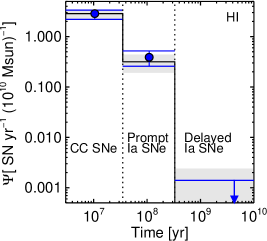
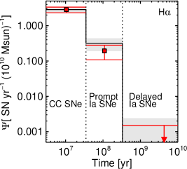
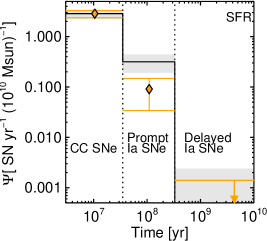
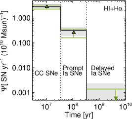
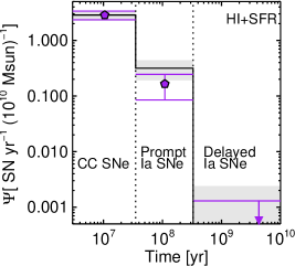
Figure 1: Best-fit delay-time distributions for the Magellanic Cloud SNR sample. Each panel in the top row displays the results obtained with a different density tracer: HI (left), H$\alpha$ (centre), and SFR (right). The panels in the bottom row show the DTDs obtained with “hybrid” density tracers, using HI at low densities and either H$\alpha$ (left) or SFR (right) at high densities. Error bars show 68% confidence intervals, from Monte-Carlo simulations that account both for Poisson statistics and for the uncertainties in the SFR of each cell. The best fits in the most-delayed bins are always zero, and the horizontal line gives the 95% confidence upper limit on the rate in this time bin. To facilitate comparison, the DTD obtained without scaling with density of the visibility time of SNRs is plotted in all panels as black lines, with shaded regions for the error bars. All DTDs have been scaled so as to give the same, theoretically expected, CC-SN yield in the first bin.

Figure 1 and Table 2 show the Magellanic Cloud DTD we recover from the SNR sample, binning the DTD into the following three intervals: $\tau<35$ Myr (CC SNe), $35~{}{\rm Myr}<\tau<330$ Myr (“prompt” SNe Ia) and $330~{}{\rm Myr}<\tau<14$ Gyr (“delayed” SNe Ia). The small number of SNe in our “survey” precludes the possibility of finer binning and a detailed recovery of the DTD shape. Nevertheless, we will see that some interesting results emerge even with this coarse binning scheme.

6.2 Core-collapse SNe

For each of the density tracers, we renormalise the visibility time at the mean density, $t_{\rm max,0}$, such that the rate in the first DTD bin, which traces CC-SNe, is $\Psi_{1}=2.86~{}{\rm SNe~{}yr}^{-1}(10^{10}M_{\odot})^{-1}$. Multiplied by the width of the bin, 35 Myr, this then gives a time-integrated CC-SN yield (i.e., the number of CC-SNe per unit stellar mass formed) of $N_{\rm CC}/M=0.01~{}{\rm M_{\odot}}^{-1}$. This is the value expected if all stars above $8M_{\odot}$ explode as CC SNe,

$$\frac{N_{\rm CC}}{M}=\frac{\int_{8}^{100}(dN/dm)dm}{0.7\int_{0.1}^{100}m(dN/dm)dm}=0.01~{}{\rm M_{\odot}}^{-1},$$ (18)

for a “diet Salpeter” IMF (Bell et al., 2003), where $dN/dm\propto m^{-2.35}$, $m$ is stellar mass in units of ${M_{\odot}}$, and the factor 0.7 in the denominator accounts for the reduced number of low-mass stars in a realistic IMF, compared to the original Salpeter (1955) IMF (see §2).

As listed in Table 2 for the three density tracers, the renormalized visibility time at a location in the MCs having the mean density is: 22.5 kyr (resolved SFR); 13.9 kyr (H$\alpha$); and 13.3 kyr (HI). Depending on the local value of the density, individual SNRs in the MCs could obviously be much older – at a density 10 times lower than the mean, for instance, the SNR lifetime would be a factor 3 to 4 longer, depending on the value of the exponent in Eq. 8. Our SNR lifetimes are therefore in agreement with the maximum ages of SNR shells constrained by SNR-pulsar associations ($\sim 60$ kyr, Frail et al., 1994).

Our resulting DTD will be incorrectly normalized if, in reality, the mass border between CC-SNe and SNe Ia is not at $8M_{\odot}$, or if a large fraction of massive stars end their lives without a SN explosion that leaves a remnant (e.g., through direct collapse to a black hole; Kochanek et al., 2008). However, a direct derivation by Maoz et al. (2010a) of the CC-SN DTD from the LOSS-SDSS sample supports the conclusion that the CC-SN yield is at the level assumed here.

The errors we cite in Fig. 1 and Table 2 give the 68% probability range of each component, based on Monte-Carlo simulations, as described above. In these simulations, to account also for the uncertainties given by Harris & Zaritsky (2009) and Harris & Zaritsky (2004) for their SFHs, we have done the following. For each MC cell, we add in quadrature the $1\sigma$ errors in SFH among the fine time bins that constitute a single co-added time bin in our analysis. Since there is covariance among the SFH errors in adjoining bins, this addition constitutes a conservative overestimate of the true errors. Then, in every mock survey in the simulation, we draw, for each cell in every time bin, a SFR from an asymmetric Gaussian distribution, centered on the Harris & Zaritsky (2009) and Harris & Zaritsky (2004) best-fit value, with positive and negative standard deviations according to the bin-added negative and positive errors above. After calculation of the expectation value of the rate for the cell, according to Eq. 12, the “observed” number of SNRs in the cell is drawn from the appropriate Poisson distribution. An exception to this procedure is in the SMC, where we have avoided using the $1\sigma$ positive errors of Harris & Zaritsky (2004), as they are two orders of magnitude larger than those given by Harris & Zaritsky (2009) for the LMC, despite the similarity between the two galaxies, their data, and their analysis. For the SMC, we therefore use the negative errors in the SFH to represent the positive errors as well. Finally, in the DTD reconstruction of each mock survey, the Harris & Zaritsky (2004, 2009) best-fit value is assumed for the SFH (i.e., a value generally different than what was used to generate the mock survey).

We note that, although we have renormalized $t_{\rm max,0}$, so as to always obtain $\Psi_{1}=2.86~{}{\rm SNe~{}yr}^{-1}(10^{10}M_{\odot})^{-1}$, $\Psi_{1}$ is still a parameter in the DTD reconstruction, and its derived error indicates the confidence level at which a CC-SN component is detected in the DTD. For the different density tracers, the $\Psi_{1}$ component of the DTD is detected in our reconstruction at the $5-7\sigma$ level. In other words, there is no doubt that some of the SNRs in the MCs are significantly associated with stellar populations that are young enough to produce CC-SNe.

Table 2: Mean SNR Visibility times, SN rates, and reconstructed DTDs from the MC SNR sample.

Density	Mean SNR	SN Rate		$\Psi_{i}$ [$\rm{SNe~{}yr^{-1}}\,(10^{10}\,\rm{M_{\odot}})^{-1}$]
Tracer	Visibility			$\Psi_{1}$	$\Psi_{2}$		$\Psi_{3}$
	[kyr]	[$10^{-3}$ SN yr-1]	[SNuM]	0-35 Myr	35-330 Myr	(95% low lim.)	0.33-14 Gyr
HI	13.3	$4.1\pm 0.9$	$3.0\pm 0.7$	$2.86^{+0.66}_{-0.50}$	$0.389\pm 0.131$	($>0.171$)	$<0.0014$
SFR (Schmidt law)	22.5	$2.4\pm 0.4$	$1.7\pm 0.3$	$2.86^{+0.50}_{-0.43}$	$0.091\pm 0.057$	($>0.016$)	$<0.0014$
H$\alpha$ (Schmidt law)	13.9	$3.3\pm 0.6$	$2.3\pm 0.4$	$2.86^{+0.54}_{-0.50}$	$0.194\pm 0.086$	($>0.060$)	$<0.0016$
No Scaling	13.4	$5.8\pm 0.1$	$3.5\pm 0.7$	$2.86^{+0.61}_{-0.50}$	$0.316\pm 0.125$	($>0.143$)	$<0.0024$
HI+H$\alpha$	12.6	$3.8\pm 0.8$	$2.6\pm 0.5$	$2.86^{+0.57}_{-0.52}$	$0.260\pm 0.100$	($>0.104$)	$<0.0014$
HI+SFR	15.9	$3.1\pm 0.6$	$2.1\pm 0.4$	$2.86^{+0.51}_{-0.51}$	$0.165\pm 0.080$	($>0.058$)	$<0.0013$

SN rates in units of SN yr^-1 are for the LMC and SMC together. SN rates per unit stellar mass are in SNuM [SNe $(100~{}{\rm yr})^{-1}(10^{10}M_{\odot})^{-1}]$, after converting formed mass to present mass, by assuming 30% mass loss. Quoted numbers are: best-fit values and 68% confidence intervals for the rates, $\Psi_{1}$ and $\Psi_{2}$; 95% confidence lower limits for $\Psi_{2}$; and 95% confidence upper limits for $\Psi_{3}$.

6.3 Prompt SNe Ia

The strong DTD signal recovered in the CC bin effectively “uses up” much of the SN data in the survey, leaving a weaker signal in the SN Ia bins. Nevertheless, there is a signal in the “prompt” SN Ia bin, $\Psi_{2}$, at 35 Myr$<\tau<330$ Myr, at the $1.7\sigma$ level for the resolved star formation tracer, $2.3\sigma$ for the H$\alpha$ tracer, and $3\sigma$ when using HI column as the density tracer. The rate $\Psi_{2}$ itself is also correspondingly higher or lower when using each of these tracers, as shown in Table 2. Here, by “$X\sigma$” we mean the number of $-34\%$ uncertainty intervals above zero. Because of the non-Gaussian nature of the errors, the significance of the detection is higher that it would be for the same number of standard deviations in a Gaussian. Specifically, we find from Monte-Carlo simulations, in which we input a value of $\Psi_{2}=0$, that recovered values as high as the best-fit values are obtained in fewer that 1% of mock surveys, using any of the tracers. In other words, a nonzero prompt SN Ia component is detected at $>99\%$ confidence. Using additional simulations, we have determined, for each tracer, the input $\Psi_{2}$ rate that gives recovered $\Psi_{2}$ values greater of equal to the best-fit values in 5% of the realizations. This input $\Psi_{2}$ rate is the 95% confidence lower limit on $\Psi_{2}$, which is also listed in Table 2. Despite the clear detection of a prompt SN Ia component, there is factor 4 systematic uncertainty in the best-fit amplitude of this component. This stems from the systematic uncertainty in estimating the local density, which in turn leads to an uncertainty in the scaling of the visibility time.

The $\Psi_{2}$ rate, multiplied by the length of the second time bin (295 Myr), indicates a time-integrated production of prompt SNe Ia of: $N_{\rm Ia}/M=0.0027\pm 0.0014~{}{\rm M_{\odot}}^{-1}$ (resolved SFR); $N_{\rm Ia}/M=0.0057\pm 0.0026~{}{\rm M_{\odot}}^{-1}$ (H$\alpha$); or $N_{\rm Ia}/M=0.0114\pm 0.0039~{}{\rm M_{\odot}}^{-1}$ (HI). We note that $N_{\rm Ia}/M$, above, is essentially the “$B$ parameter” discussed by Scannapieco & Bildsten (2005), Mannucci et al. (2006), and Sullivan et al. (2006), i.e., the ratio of SN Ia rate to SFR in strongly star-forming galaxies. As summarised in Maoz (2008), the values of $B$ generally found by SN surveys are in the range $B=0.001$ to $0.003~{}{\rm M_{\odot}}^{-1}$, an exception being Sullivan et al. (2006), who obtain a value several times lower, $(3.9\pm 0.7)\times 10^{-4}{\rm M_{\odot}}^{-1}$. The values we find for $N_{\rm Ia}/M$ are broadly consistent with those estimates, but tend to be on the high side, particularly when we use HI column as a density tracer in the MCs.

The time-integrated ratio of CC-SNe to SNe Ia (or equivalently, the ratio of rates of CC and type-Ia SNe in a population that has had a constant star-formation rate for a long time, such that both rates have reached a steady state) is in the range of $9:1$ to $1:1$, when we consider both the statistical and the systematic uncertainties.

6.4 Delayed SNe Ia

The DTD amplitude in the third bin has a best-fit value of zero in all of our reconstructions, but an uncertainty range that includes the typical SN Ia rates that have been measured in old, quiescent populations. The uncertainty is large because few SNe are expected in this bin in our small sample, given the dominance of young stellar populations in the MCs. Specifically, from our Monte-Carlo simulations, the $95\%$ confidence upper limit on the delayed SN Ia rate in the DTD is $\Psi_{3}<0.0013~{}{\rm to}~{}0.0016$ SNe yr${}^{-1}(10^{10}M_{\odot})^{-1}$ (depending on the density tracer). In other words, such an input value in the simulations for this component of the DTD results in a best-fit reconstructed value of zero in 5% of cases. For comparison, the typical values found for the “$A$ parameter”, the SN Ia rate per unit mass in an old population that has no ongoing star formation, have been in the range $A\sim(2-10)\times 10^{-4}$ SNe yr${}^{-1}(10^{10}M_{\odot})^{-1}$ (see compilation in Maoz, 2008). However, $\Psi_{3}$ is the rate per unit mass formed. The published rates in old populations are a per unit of existing stellar mass, i.e., in stars and stellar remnants. In the course of $\sim 10$ Gyr, a stellar population (with a “diet Salpeter” IMF that we are assuming throughout) will return $\approx 50\%$ of its mass to the interstellar medium via SN explosions and mass loss during stellar evolution (Bruzual & Charlot, 1993). Thus, for comparison to $\Psi_{3}$, $A$ needs to be multiplied by $0.5$, giving $\sim(1-5)\times 10^{-4}$ SNe yr^-1 per $(10^{10}M_{\odot})^{-1}$ formed. This range fits comfortably, by at least a factor of 2, below the upper limit we have derived here based on the SNRs in the MCs. An application of our DTD recovery method to the LOSS SN survey, which does have a significant old galaxy population, by Maoz et al. (2010a), gives a highly significant measurement of a delayed SN Ia component, $\Psi_{3}=2.6^{+0.8}_{-0.6}\times 10^{-4}$ SNe yr${}^{-1}(10^{10}M_{\odot})^{-1}$. This value is consistent both with previous determinations of the $A$ parameter and with the upper limit on $\Psi_{3}$ found here.

6.5 Relative fraction of prompt and delayed SNe Ia

Bins 2 and 3 of the DTD thus, respectively, require the existence of prompt SNe Ia, and allow (but do not require) the existence also of a delayed component. We note that, if we choose to ignore the density distribution, and assume a constant visibility time throughout the MCs, we obtain results that are intermediate to those using H$\alpha$ and HI, in terms of visibility time and prompt-SN-Ia significance and amplitude, and hence also in terms of SN Ia yield and CC-SN to SN Ia time-integrated ratio.

We can also use the $\Psi_{2}$ measurements and the upper limits on $\Psi_{3}$ to gauge the relative fraction of the prompt and delayed SNe among the SN Ia population. Using the resolved-SFR-based values of $\Psi_{2}$ and $\Psi_{3}$ in Table 2, which have the lowest ratio, we can obtain a lower limit on the time-integrated SN Ia yields in the two components,

$$\frac{\Psi_{2}\Delta t_{2}}{\Psi_{3}\Delta t_{3}}\gtrsim 1,$$ (19)

wher $\Delta t_{2}$ and $\Delta t_{3}$ are the sizes of time-bins 2 and 3. Using the other tracers gives lower limits on this ratio that are larger. In any case, a significant fraction of SNe Ia, possibly a majority, are prompt.

6.6 Hybrid density tracers

Among the three density tracers that we use, the HI column density is physically closest to the actual volume density we are interested in. Furthermore, it can probe and represent the lower-density regions of the MCs, where the two other tracers, which rely on an inverse Schmidt law, break down because of the mass column threshold in the SFR. In those low-density regions, we have knowingly assigned a constant, artificially high, density which systematically shortens the visibility time. Finally, the Schmidt law has a large intrinsic scatter, inducing noise in the assignment of visibility times. If we focus on the HI-tracer results, we find a highly significant prompt-SN-Ia component, with an amplitude somewhat higher than found by field SN surveys, and a time-integrated ratio of CC-SNe to SNe Ia of approximately 1:1. Interestingly, by looking at this ratio for the youngest remnants in the LMC, which are the ones that can be most securely classified, one would have guessed as much – four of the eight smallest SNRs in the LMC were definitely or likely type Ia’s (Badenes et al., 2009a).

On the other hand, HI as a density tracer also has its shortcomings. For example, the cell in the centre of the 30 Doradus region of the LMC has a high SFR, as evidenced by its resolved mean SFR over the last 35 Myr, which is 5 times higher than the mean of the MCs, and by its H$\alpha$ luminosity, which is 30 times higher than the mean. The HI column density, however, is only twice as high as the mean for the MCs. Harris & Zaritsky (2009) have already noted the far-from-perfect spatial correlation amongst different tracers of star formation. In the case of 30 Doradus, the HI column is likely underestimating the true total gas density, because a fraction of the neutral hydrogen has been photoionised by the massive stars in this region. An underestimate of gas density in such regions will lead to an overestimate of the visibility time. This, in turn, will lower $\Psi_{1}$, the DTD rate of CC-SNe that are associated with such regions. Renormalising the entire DTD such that $\Psi_{1}=2.86$ will then lift also the prompt-SN-Ia component, $\Psi_{2}$, causing its rate to be overestimated. At some level, this is likely occurring when we use HI column as a density tracer. Furthermore, we have discussed in Paper I the evidence that HI may be misrepresenting the density in the SMC because of projection effects. Thus, this tracer is also not foolproof.

To deal with these problems, we have combined two different tracers, using each in the regime where it is likely to be most reliable. We have rederived the visibility time in each cell, using HI column as the density tracer in cells where the column density is lower than the mean (about 2/3 of the cells), and using SFR and the inverse Schmidt law, as before, in the rest of the cells, where HI is above the mean. The SFR is traced either with the resolved stellar populations, or using H$\alpha$.

The best-fit DTD recovered with these visibility times (see Table 2), not surprisingly, is intermediate to the ones found with HI and H$\alpha$ or the resolved SFR when used alone as tracers. The prompt SN Ia component is detected at a level of $2.6\sigma$ above zero (using HI + H$\alpha$) or $2.1\sigma$ above zero (using HI + resolved SFR). As before, from the Monte Carlo simulations, the significance of these detections is $>99\%$. The results do not depend strongly on the adopted border for the use of the two tracers. For example, setting the border between use of HI and resolved SFR at 1/2 of the mean HI column or at twice the mean HI column (instead of at the mean), changes the best-fit value of $\Psi_{2}$ by $-27\%$ and $+20\%$, respectively. We consider these hybrid-tracer-based DTDs to be our most reliable results.

6.7 Sensitivity to temporal binning and leaks

A concern with all of our results is that they may be sensitive to the temporal border between CC-SNe and SNe Ia, which we have set at 35 Myr. For example, if some CC-SNe explode, say, between 35 Myr and 45 Myr, some of the CC-SN signal will be attributed incorrectly to SNe Ia. As a result, we will overestimate the number of prompt SNe Ia. To test this possibility, we have performed the following experiment. We have selected 11 LMC SNRs from Paper I that are almost certainly remnants of CC explosions, based on one or more of the following criteria: detection of pulsars within them, X-ray analysis of the ejecta showing clear CC-SN products, or (in the case of SN1987A) direct historical evidence. With this small sample of known CC-SNe, which we list in Table 3, we have re-derived the DTD. Naturally, the amplitude of the shortest, CC-SN, bin of the DTD will be understimated, because we have selected only a fraction of the CC remnants in the LMC. Nevertheless, we can test if any signal “leaks” into the later bins, which we have been associating with SNe Ia, either because of the time border issue discussed above, or because of some other systematics of the Harris & Zaritsky (2009) SFH reconstruction. We find no evidence of “leakage” outside the $<35$ Myr bin. For example, using the HI+H$\alpha$ hybrid density tracer, the best-fit results are, in the first (earliest) time bin of the DTD (with no renormalisation of this rate), $\Psi_{1}=0.61\pm 0.26$ SNe yr${}^{-1}(10^{10}M_{\odot})^{-1}$, and zero in the second and third bins. This is reassuring, but because of the small size of this subsample, the 95% confidence upper limit on the rates in the second and third bins are not low enough to rule out, using this test, a leak of the CC signal, having the amplitude of the second and third bins in the full sample.

As another test, we have rederived the full-sample DTDs with the various tracers, but enlarging the first time bin from 0-35 Myr to 0-80 Myr (this step size is dictated by the time bins of the Harris and Zaritsky SFH reconstructions). Not surprisingly, the best-fit amplitude of $\Psi_{2}$ decreases by factors of 2-3, comparable to the increase in the length of the first time bin. Unfortunately, the relative uncertainty in $\Psi_{2}$ also becomes very large, precluding the possibility of saying with any confidence whether or not a SN Ia component at delays of 80-330 Myr exists. However, it is highly unlikely that, at 80 Myr delays, there are still contributions to the DTD from CC-SNe, as this delay corresponds to the lifetime of stars with initial masses below $6M_{\odot}$. Thus, this exercise suggests that much of the signal in the 35-330 Myr bin of the DTD could be due to SNe Ia that explode within $<80$ Myr. This result joins other evidence for prompt SNe Ia with extremely short delays, of $\lesssim 100$ Myr (Mannucci et al., 2006, ; Della Valle et al. 2005). The obstacle to obtaining a clearer answer, however, is the small number of SNRs. One needs to recall that, among the 77 SNRs in our sample, at most half and possibly only about 10% are ”driving” the SN Ia signals in the second and third DTD bins, and hence the large uncertainty. A larger sample of SNRs could be obtained by combining SNRs from several nearby galaxies, as briefly discussed in §8, below.

Table 3: Bona fide CC-SNRs in the LMC

SNR	Alternate	CC Classification
	Name	Criteria and Reference
J0453.6$-$6829	B0453$-$685	NS; Gaensler et al. (2003)
J0505.9$-$6802	N23	NS; Hughes et al. (2006)
J0525.1$-$6938	N132D	EJ; Borkowski et al. (2007)
J0525.4$-$6559	N49B	EJ; Park et al. (2003b)
J0526.0$-$6604	N49	EJ; Park et al. (2003a)
J0531.9$-$7100	N206	NS; Williams et al. (2005)
J0535.5$-$6916	SNR1987A	historical CC-SN
J0535.7$-$6602	N63A	EJ; Warren et al. (2003)
J0536.1$-$6734	DEM L241	NS; Bamba et al. (2006)
J0537.8$-$6910	N157B	NS; Chen et al. (2006)
J0540.2$-$6919	B0540-693	NS; Kirshner et al. (1989)

6.8 Comparison of the visibility time to theoretical estimates

An interesting question that we can ask, at this point, is how do the observed values of visibility time that we have obtained compare to the theoretical expectations for the age at the SNR transition to the radiative phase. Blondin et al. (1998) found, using 1D hydrodynamical simulations and a full cooling curve (rather than a power-law approximation) that the transition time is well approximated by $1.6~{}t_{\rm cool}$ for a wide range of conditions, where $t_{\rm cool}$ is their rough estimate for the cooling time, as in our Eqns. 4 and 7, assuming a cooling function represented by an $\epsilon=-1$ power law. Specifically, they found that for an ambient hydrogen number density of $1~{}{\rm cm}^{-3}$, and for the fiducial explosion energy and gas abundances, $t_{\rm cool}\approx 29$ kyr, and hence the theoretical transition time for this density is $t_{\rm max}\approx 29\times 1.6=46$ kyr.

Unfortunately, we cannot directly compare this number to the visibility times we have obtained in this work, using the various density tracers. Our tracers are all based on column densities, rather than densities, under the assumption that the two are correlated. For example, although we know that for the mean HI column density of the clouds, $1.5\times 10^{21}{\rm cm}^{-2}$, the visibility time is 13.3 kyr (using HI as a tracer), we do not know what absolute density this corresponds to. Therefore, neither do we know how to scale the visibility time to its value for the fiducial Blondin et al. (1998) density of $1~{}{\rm cm}^{-3}$.

Instead, we will check if the LMC disk thickness needed in order to match the numbers is reasonable. Assuming a visibility-time dependence on density of $t_{\rm max}\propto\rho^{-1/2}$, our observed range of $t_{\rm max}=13.3$ to 22.5 kyr implies a mean density of $n\sim[46/(13.3~{}{\rm to}~{}22.5)]^{2}\approx 4~{}{\rm to}~{}12~{}{\rm cm}^{-3}$. We note that, although Blondin et al. (1998) consider the case of a shock expanding into a neutral hydrogen ambient medium, the results would change little if the ambient medium consisted of molecular hydrogen, or a mixture of neutral and molecular hydrogen. The 21 cm emission traces only the atomic hydrogen, while molecular hydrogen is present in the gas disk as well. Norikazu et al. (2001) have used CO as a molecular gas tracer to measure a molecular-to-atomic mass ratio of $0.2:1$ in the low-radial velocity component of the gas in the LMC disk, associated with the densest regions. However, for low columns or low metallicities, CO may no longer be a be a good tracer, because it can be photodissociated whereas H₂ remains self-shielded (Leroy et al. 2009), and the actual molecular ratio is likely higher. Thus, it is reasonable to assume that the total gas column density is at least $\approx 2\times 10^{21}{\rm cm}^{-2}$. Dividing by $n$ then gives a LMC gas disk thickness of about 60 to 170 pc or more, smaller than, but comparable to the 300 pc-thick Milky Way gas disk. We conclude that, while there is too much missing information about the LMC geometry (and certainly about that of the SMC) for a definitive test of the Blondin et al. (1998) model and its application by us to SNR visibility, there appears to be rough consistency in the numbers.

7 The Current SN Rate

We have focused, up to this point, on deriving the SN DTD, which has permitted us to separate, based on delay times, the contributions of CC-SNe, prompt SN Ia, and delayed SNe Ia. However, the data allow deriving also the more traditional current SN rate in the MCs, which is also of interest. Naturally, the rates we will get will be total rates, for all types of SNe, CC and type-Ia, that produce SNRs. The SN rate in the LMC or SMC, or in both galaxies treated as a whole, will simply be

$$R=\frac{N_{\rm SNR}N_{\rm cells}}{\sum_{i}t_{i}},$$ (20)

where $N_{\rm SNR}$ is the total number of remnants, $N_{\rm cells}$ is the number of cells, and the sum over the visibility times, $t_{i}$, is over all cells. Alternatively, one can calculate the SN rate per unit mass,

$$R_{M}=\frac{N_{\rm SNR}}{\sum_{i}m_{i}t_{i}},$$ (21)

where $m_{i}$ is the time-integrated stellar mass formed in each cell (i.e., $m_{i}=\sum_{j}m_{ij}$). The relative error in these rates is given by the sum in quadrature of the relative Poisson error, $N_{\rm SNR}^{-1/2}$, and the relative error of the visibility time. Since all the visibility times have been renormalised to give $\Psi_{1}=2.86$, the relative visibility-time error is just the relative error in $\Psi_{1}$. Measurements of $R_{M}$ in other galaxies have generally been normalised not to the formed stellar mass, but to the existing stellar mass. For ease of comparison to those measurements, we will therefore scale down all values of $m_{i}$ by 0.7, which accounts roughly for the mass loss of stars during stellar evolution in actively star-forming galaxies like the MCs (Bruzual & Charlot, 1993). (This 30% mass loss is in contrast to the 50% mass loss previously considered for old and quiescent stellar populations). Rates per unit mass in Table 2 are in units of SNuM [SNe $(100~{}{\rm yr})^{-1}(10^{10}M_{\odot})^{-1}$].

As with our derivation of the DTD, we will get different rates, depending on the density tracer we use. Table 2 lists, for each of the density tracers, and for the hybrid combinations, the values or $R$ and $R_{M}$ in the MCs as a whole. Considering the range in $R$ covered by the uncertainties and by the different tracers, we see that a SN explodes in the MCs once every 200 to 500 years. This is in excellent agreement with the historical record: the two most recent SNe in the MCs were SN1987A (a CC-SN), and SNR J0509.5$-$6731 (B0509$-$67.5) which exploded circa 1600 and was a SN Ia [(Rest et al., 2008); see §5.3 of (Badenes et al., 2008)]. It is highly implausible that many additional SNe exploded in the MCs over the past 400 years but were unnoticed by naked-eye observers.

In terms of mass-normalised SN rates, the range encompassing the different tracers and their $1\sigma$ uncertaities, 1.7 to 3.7 SNuM, is in excellent agreement with rates measured in the bluest dwarf galaxies, of which the MCs are prototypes. For such galaxies, which have the highest-known mass-normalised SN rates, (Mannucci et al., 2005) have measured rates, in SNuM, of $2.3\pm 0.8$ (CC-SNe) and $0.9\pm 0.4$ (SNe Ia), or a total SN rate of $3.2\pm 0.9$ SNuM.

Conversely, we can use the above SN rates to reinforce our claim that that SNR sample we compiled in Paper I is indeed fairly complete, and that our model, in which the MC SNRs are in their Sedov-Taylor phase, is correct. Suppose, by way of negation, that the MC SNRs are actually in free expansion, as has been invoked by a number of authors to explain the observed uniform SNR size distribution (see Paper I). Since free-expansion SNR shock velocities are in the range $\sim 5000$ to 10,000 km s^-1, the maximum observed SNR radii of $r\sim 30$ pc would translate to maximum ages of 3 to 6 kyr. The 77 SNRs in the MCs would then imply a SN explosion in the MCs once every 40 to 80 years, on average, or even more frequently if our SNR sample is incomplete. Similarly, the 3 to 6 kyr visibility time, independent of ambient density in this picture, would give mass normalised total SN rates of 8 to 15 SNuM, or even higher if our sample is incomplete. This is much higher than in any known type of galaxy. Most seriously, perhaps, if the visibility time were fixed at, say, 6 kyr, this would raise $\Psi_{1}$ in the “no scaling” model of Table 2 from a value of 2.86 to $6.4~{}{\rm SNe~{}yr^{-1}}~{}(10^{10}~{}M_{\odot})^{-1}$, corresponding to a CC-SN yield of $0.022~{}M_{\odot}^{-1}$. To produce so many CC-SNe with any standard IMF, all stars with initial mass above $3.7M_{\odot}$ would have to undergo core-collapse. This is in direct contradiction to stellar evolution theory, and to the semi-empirical initial-final mass relation for WDs (e.g. (Catalán et al., 2008; Salaris et al., 2009; Williams et al., 2009))

In summary, the Sedov model we have adopted to explain the MC SNR size distribution is consistent with the gas density distributions of the MCs (Paper I), and results in MC SN rates that are consistent with the historical record and with the rates measured in similar types of galaxies. In contrast, a free-expansion model for the MC SNRs produces rates that are in stark contradiction with these observations, and with expectations from stellar evolution.

8 Summary and Conclusions

In Paper I, we assembled a multi-wavelength compilation of the 77 known SNRs in the MCs, collected from the existing literature. We verified that this compilation is fairly complete, and that the size distribution of SNRs is approximately flat, within the allowed uncertainties, up to a cutoff at $r\sim 30$ pc, as noted by other authors before. We then proposed a physical model to explain this size distribution. According to our model, most of the SNRs are in their Sedov stage, quickly fading below detection as soon as they reach the radiative stage. Under these circumstances, a flat distribution of SNR sizes can be obtained, provided that the distribution of densities in the MCs follows a power law with index $-1$. Finally, in Paper I, we used three different density tracers (HI column density, H$\alpha$ flux, and SFR) to demonstrate that the distribution of densities in the MCs indeed follows a power law of index $-1$.

In this paper, we have used the Paper I sample of SNRs as an effective supernova survey, conducted over tens of kyr. We have applied a novel technique to this SNR sample to derive, in these galaxies, the SN rates and the SN DTD. In order to accomplish this, we have used the three tracers of the density to scale the visibility time of SNRs in the MCs. From the scaled visibility times and the SFH maps from the resolved stellar populations in the MCs published by Harris & Zaritsky (2004) and Harris & Zaritsky (2009), we have calculated the DTD. The DTDs we have derived are the first obtained using SFHs from resolved stellar populations.

Our main findings are the following:
1. We detect at the $>99\%$ confidence level a “prompt” SN Ia population, defined here as one that explodes within 330 Myr of star formation. This finding joins a growing number of measurements of such a component (see §1). However, our measurement is based on our statistically robust DTD recovery method, with its avoidance of the averaging inherent to many previous measurements, and using the most reliable SFHs, based on resolved stellar populations. The yield of prompt SN Ia, in terms of SNe per stellar mass formed, is also consistent with other measurements.
2. We obtain upper limits on the delayed SN Ia population, which are consistent with other measurements. Using these upper limits, we find that roughly half, but possibly more, of SNe Ia are “prompt”, as defined above. This again joins previous results on the large relative fraction of the prompt population.
3. We use our SNR sample and our SNR visibility times to derive current MC SN rates. The SN rate in the MCs agrees well with the historical record for these galaxies. The mass-normalised SN rate in the MCs is in excellent agreement with the rates measured by SN surveys in galaxies of this type. This lends support to the physical model we have presented to explain the SNR size distribution and the clouds, and which we have used to derive visibility times for our DTD and rate calculations.
4. Conversely, a “free expansion” model for the SNRs, as has been invoked for the MCs and other galaxies, would imply SN rates in conflict with the historical record and with the rates in other star-forming dwarf galaxies. Furthermore, this model would indicate an unreasonably high yield of CC-SNe per stellar mass formed.

The main limitation of our study has been the relatively small number of SNRs in the MC sample, which has forced us to use coarse time bins and has led to large Poisson errors. Construction of significantly larger samples of SNRs is, however, possible by means of deep radio surveys of additional galaxies that are near enough for deriving SFHs of their individual regions via resolved stellar populations, namely M31 and M33 (see Paper I). Such data would permit a similar analysis to the one we have done, but with larger SNR numbers, permitting a more accurate determination of the SN DTD, and bringing into better focus the properties of SNe, their remnants, and the connections between them.

References

- Aubourg et al. (2008) Aubourg É., Tojeiro R., Jimenez R., Heavens A., Strauss M. A., Spergel D. N., 2008, A&A, 492, 631
- Badenes et al. (2009a) Badenes C., Harris J., Zaritsky D., Prieto J. L., 2009a, ApJ, 700, 727
- Badenes et al. (2008) Badenes C., Hughes J. P., Cassam-Chenaï G., Bravo E., 2008, ApJ, 680, 1149
- Badenes et al. (2009b) Badenes C., Mullally F., Thompson S. E., Lupton R. H., 2009b, ApJ, 707, 971
- Bamba et al. (2006) Bamba A., Ueno M., Nakajima H., Mori K., Koyama K., 2006, A&A, 450, 585
- Barris & Tonry (2004) Barris B. J., Tonry J. L., 2004, ApJ, 613, L21
- Bear & Soker (2009) Bear E., Soker N., 2009, ArXiv e-prints
- Beer et al. (2007) Beer M. E., Dray L. M., King A. R., Wynn G. A., 2007, MNRAS, 375, 1000
- Bell et al. (2003) Bell E. F., McIntosh D. H., Katz N., Weinberg M. D., 2003, ApJS, 149, 289
- Bigiel et al. (2008) Bigiel F., Leroy A., Walter F., Brinks E., de Blok W. J. G., Madore B., Thornley M. D., 2008, AJ, 136, 2846
- Blondin et al. (1998) Blondin J. M., Wright E. B., Borkowski K. J., Reynolds S. P., 1998, ApJ, 500, 342
- Borkowski et al. (2007) Borkowski K. J., Hendrick S. P., Reynolds S. P., 2007, ApJ, 671, L45
- Brandt et al. (2010) Brandt T. D., Tojeiro R., Aubourg É., Heavens A., Jimenez R., Strauss M. A., 2010, ArXiv e-prints
- Bruzual & Charlot (1993) Bruzual A., Charlot S., 1993, ApJ, 405, 538
- Cassisi et al. (1998) Cassisi S., Iben I., Tornambé A., 1998, ApJ, 496, 376
- Catalán et al. (2008) Catalán S., Isern J., García-Berro E., Ribas I., 2008, MNRAS, 387, 1693
- Chen et al. (2006) Chen Y., Wang Q. D., Gotthelf E. V., Jiang B., Chu Y., Gruendl R., 2006, ApJ, 651, 237
- Cioffi et al. (1988) Cioffi D. F., McKee C. F., Bertschinger E., 1988, ApJ, 334, 252
- Cooper et al. (2009) Cooper M. C., Newman J. A., Yan R., 2009, ApJ, 704, 687
- Dahlen et al. (2008) Dahlen T., Strolger L., Riess A. G., 2008, ApJ, 681, 462
- Dahlen et al. (2004) Dahlen T., Strolger L., Riess A. G., Mobasher B., Chary R., Conselice C. J., Ferguson H. C., Fruchter A. S., Giavalisco M., Livio M., Madau P., Panagia N., Tonry J. L., 2004, ApJ, 613, 189
- Di Stefano (2010) Di Stefano R., 2010, ApJ, 712, 728
- Dilday et al. (2010) Dilday B., Bassett B., Becker A., Bender R., Castander F., Cinabro D., Frieman J. A., Galbany L., Garnavich P., Goobar A., Hopp U., Ihara Y., Jha S. W., Kessler R., Lampeitl H., Marriner J., Miquel R., Mollá M., Nichol R. C., Nordin J., Riess A. G., Sako M., Schneider D. P., Smith M., Sollerman J., Wheeler J. C., Östman L., Bizyaev D., Brewington H., Malanushenko E., Malanushenko V., Oravetz D., Pan K., Simmons A., Snedden S., 2010, ArXiv e-prints
- Eisenhardt et al. (2008) Eisenhardt P. R. M., Brodwin M., Gonzalez A. H., Stanford S. A., Stern D., Barmby P., Brown M. J. I., Dawson K., Dey A., Doi M., Galametz A., Jannuzi B. T., Kochanek C. S., Meyers J., Morokuma T., Moustakas L. A., 2008, ApJ, 684, 905
- Eldridge et al. (2008) Eldridge J. J., Izzard R. G., Tout C. A., 2008, MNRAS, 384, 1109
- Förster et al. (2006) Förster F., Wolf C., Podsiadlowski P., Han Z., 2006, MNRAS, 368, 1893
- Frail et al. (1994) Frail D. A., Goss W. M., Whiteoak J. B. Z., 1994, ApJ, 437, 781
- Gaensler et al. (2003) Gaensler B. M., Hendrick S. P., Reynolds S. P., Borkowski K. J., 2003, ApJ, 594, L111
- Gaensler & Johnston (1995) Gaensler B. M., Johnston S., 1995, MNRAS, 275, L73
- Gal-Yam & Maoz (2004) Gal-Yam A., Maoz D., 2004, MNRAS, 347, 942
- Gal-Yam et al. (2008) Gal-Yam A., Maoz D., Guhathakurta P., Filippenko A. V., 2008, ApJ, 680, 550
- Gal-Yam et al. (2002) Gal-Yam A., Maoz D., Sharon K., 2002, MNRAS, 332, 37
- Gaustad et al. (2001) Gaustad J. E., McCullough P. R., Rosing W., Van Buren D., 2001, PASP, 113, 1326
- Gilfanov & Bogdán (2010) Gilfanov M., Bogdán Á., 2010, Nature, 463, 924
- Girardi et al. (2000) Girardi L., Bressan A., Bertelli G., Chiosi C., 2000, A&AS, 141, 371
- Graham et al. (2009) Graham M. L., Pritchet C. J., Sullivan M., Howell D. A., Gwyn S. D. J., Astier P., Balland C., Basa S., Carlberg R. G., Conley A., Fouchez D., Guy J., Hardin D., Hook I. M., Pain R., Perrett K., Regnault N., Rich J., Balam D., Fabbro S., Hsiao E. Y., Mourao A., Palanque-Delabrouille N., Perlmutter S., Ruhlman-Kleider V., Suzuki N., Fakhouri H. K., Walker E. S., 2009, ArXiv e-prints
- Greggio et al. (2008) Greggio L., Renzini A., Daddi E., 2008, MNRAS, 388, 829
- Han & Podsiadlowski (2004) Han Z., Podsiadlowski P., 2004, MNRAS, 350, 1301
- Harris & Zaritsky (2001) Harris J., Zaritsky D., 2001, ApJS, 136, 25
- Harris & Zaritsky (2004) —, 2004, AJ, 127, 1531
- Harris & Zaritsky (2009) —, 2009, AJ, 138, 1243
- Heger et al. (2003) Heger A., Fryer C. L., Woosley S. E., Langer N., Hartmann D. H., 2003, ApJ, 591, 288
- Hernández et al. (2009) Hernández J. I. G., Ruiz-Lapuente P., Filippenko A. V., Foley R. J., Gal-Yam A., Simon J. D., 2009, ApJ, 691, 1
- Hughes et al. (2006) Hughes J. P., Rafelski M., Warren J. S., Rakowski C., Slane P., Burrows D., Nousek J., 2006, ApJ, 645, L117
- Hurley et al. (2002) Hurley J. R., Tout C. A., Pols O. R., 2002, MNRAS, 329, 897
- Iben & Tutukov (1984) Iben I., Tutukov A., 1984, ApJS, 54, 335
- Kennicutt (1989) Kennicutt Jr. R. C., 1989, ApJ, 344, 685
- Kennicutt (1998) —, 1998, ARA&A, 36, 189
- Kerzendorf et al. (2009) Kerzendorf W. E., Schmidt B. P., Asplund M., Nomoto K., Podsiadlowski P., Frebel A., Fesen R. A., Yong D., 2009, ApJ, 701, 1665
- Kim et al. (2003) Kim S., Staveley-Smith L., Dopita M. A., Sault R. J., Freeman K. C., Lee Y., Chu Y., 2003, ApJS, 148, 473
- Kirshner et al. (1989) Kirshner R. P., Morse J. A., Winkler P. F., Blair W. P., 1989, ApJ, 342, 260
- Kobayashi et al. (2000) Kobayashi, C., Tsujimoto, T., & Nomoto, K. 2000, ApJ, 539, 26
- Kochanek et al. (2008) Kochanek C. S., Beacom J. F., Kistler M. D., Prieto J. L., Stanek K. Z., Thompson T. A., Yüksel H., 2008, ApJ, 684, 1336
- Kuznetsova et al. (2008) Kuznetsova N., Barbary K., Connolly B., Kim A. G., Pain R., Roe N. A., Aldering G., Amanullah R., Dawson K., Doi M., Fadeyev V., Fruchter A. S., Gibbons R., Goldhaber G., Goobar A., Gude A., Knop R. A., Kowalski M., Lidman C., Morokuma T., Meyers J., Perlmutter S., Rubin D., Schlegel D. J., Spadafora A. L., Stanishev V., Strovink M., Suzuki N., Wang L., Yasuda N., 2008, ApJ, 673, 981
- Leonard (2007) Leonard D. C., 2007, ApJ, 670, 1275
- Mannucci et al. (2006) Mannucci F., Della Valle M., Panagia N., 2006, MNRAS, 370, 773
- Mannucci et al. (2005) Mannucci F., Della Valle M., Panagia N., Cappellaro E., Cresci G., Maiolino R., Petrosian A., Turatto M., 2005, A&A, 433, 807
- Mannucci et al. (2008) Mannucci F., Maoz D., Sharon K., Botticella M. T., Della Valle M., Gal-Yam A., Panagia N., 2008, MNRAS, 383, 1121
- Maoz (2008) Maoz D., 2008, MNRAS, 384, 267
- Maoz & Gal-Yam (2004) Maoz D., Gal-Yam A., 2004, MNRAS, 347, 951
- Maoz et al. (2010a) Maoz D., Mannucci F., Li W., Filippenko A. V., Della Valle M., Panagia N., 2010, MNRAS, in press, ArXiv e-prints
- Mennekens et al. (2010) Mennekens, N., Vanbeveren, D., De Greve, J. P., & De Donder, E. 2010, arXiv:1003.2491
- Napiwotzki et al. (2004) Napiwotzki R., Yungelson L., Nelemans G., Marsh T. R., Leibundgut B., Renzini R., Homeier D., Koester D., Moehler S., Christlieb N., Reimers D., Drechsel H., Heber U., Karl C., Pauli E.-M., 2004, in Astronomical Society of the Pacific Conference Series, Vol. 318, Spectroscopically and Spatially Resolving the Components of the Close Binary Stars, Hilditch R. W., Hensberge H., Pavlovski K., eds., pp. 402–410
- Nelemans et al. (2005) Nelemans G., Napiwotzki R., Karl C., Marsh T. R., Voss B., Roelofs G., Izzard R. G., Montgomery M., Reerink T., Christlieb N., Reimers D., 2005, A&A, 440, 1087
- Nelemans & Tout (2005) Nelemans G., Tout C. A., 2005, MNRAS, 356, 753
- Nomoto (1982) Nomoto K., 1982, ApJ, 253, 798
- Park et al. (2003a) Park S., Burrows D. N., Garmire G. P., Nousek J. A., Hughes J. P., Williams R. M., 2003a, ApJ, 586, 210
- Park et al. (2003b) Park S., Hughes J. P., Slane P. O., Burrows D. N., Warren J. S., Garmire G. P., Nousek J. A., 2003b, ApJ, 592, L41
- Poelarends et al. (2008) Poelarends A. J. T., Herwig F., Langer N., Heger A., 2008, ApJ, 675, 614
- Poznanski et al. (2007) Poznanski D., Maoz D., Yasuda N., Foley R. J., Doi M., Filippenko A. V., Fukugita M., Gal-Yam A., Jannuzi B. T., Morokuma T., Oda T., Schweiker H., Sharon K., Silverman J. M., Totani T., 2007, MNRAS, 382, 1169
- Raskin et al. (2009) Raskin C., Scannapieco E., Rhoads J., Della Valle M., 2009, ApJ, 707, 74
- Rest et al. (2008) Rest A., Matheson T., Blondin S., Bergmann M., Welch D. L., Suntzeff N. B., Smith R. C., Olsen K., Prieto J. L., Garg A., Challis P., Stubbs C., Hicken M., Modjaz M., Wood-Vasey W. M., Zenteno A., Damke G., Newman A., Huber M., Cook K. H., Nikolaev S., Becker A. C., Miceli A., Covarrubias R., Morelli L., Pignata G., Clocchiatti A., Minniti D., Foley R. J., 2008, ApJ, 680, 1137
- Rest et al. (2005) Rest A., Suntzeff N. B., Olsen K., Prieto J. L., Smith R. C., Welch D. L., Becker A., Bergmann M., Clocchiatti A., Cook K., Garg A., Huber M., Miknaitis G., Minniti D., Nikolaev S., Stubbs C., 2005, Nature, 438, 1132
- Ruiter et al. (2009) Ruiter A. J., Belczynski K., Fryer C., 2009, ApJ, 699, 2026
- Ruiz-Lapuente et al. (2004) Ruiz-Lapuente P., Comerón F., Méndez J., Canal R., Smartt S., Filippenko A., Kurucz R., Chornock R., Foley R., Stanishev V., Ibata R., 2004, Nature, 431, 1069
- Saio & Nomoto (1985) Saio H., Nomoto K., 1985, A&A, 150, L21
- Salaris et al. (2009) Salaris M., Serenelli A., Weiss A., Miller Bertolami M., 2009, ApJ, 692, 1013
- Salpeter (1955) Salpeter E. E., 1955, ApJ, 121, 161
- Scannapieco & Bildsten (2005) Scannapieco E., Bildsten L., 2005, ApJ, 629, L85
- Schmidt (1959) Schmidt M., 1959, ApJ, 129, 243
- Sharon (2010) Sharon K., et al, 2010, ApJsubmitted
- Sharon et al. (2007) Sharon K., Gal-Yam A., Maoz D., Filippenko A. V., Guhathakurta P., 2007, ApJ, 660, 1165
- Smartt (2009) Smartt S. J., 2009, ARA&A, 47, 63
- Stanimirovic et al. (1999) Stanimirovic S., Staveley-Smith L., Dickey J. M., Sault R. J., Snowden S. L., 1999, MNRAS, 302, 417
- Strolger et al. (2004) Strolger L., Riess A. G., Dahlen T., Livio M., Panagia N., Challis P., Tonry J. L., Filippenko A. V., Chornock R., Ferguson H., Koekemoer A., Mobasher B., Dickinson M., Giavalisco M., Casertano S., Hook R., Blondin S., Leibundgut B., Nonino M., Rosati P., Spinrad H., Steidel C. C., Stern D., Garnavich P. M., Matheson T., Grogin N., Hornschemeier A., Kretchmer C., Laidler V. G., Lee K., Lucas R., de Mello D., Moustakas L. A., Ravindranath S., Richardson M., Taylor E., 2004, ApJ, 613, 200
- Sullivan et al. (2006) Sullivan M., Le Borgne D., Pritchet C. J., Hodsman A., Neill J. D., Howell D. A., Carlberg R. G., Astier P., Aubourg E., Balam D., Basa S., Conley A., Fabbro S., Fouchez D., Guy J., Hook I., Pain R., Palanque-Delabrouille N., Perrett K., Regnault N., Rich J., Taillet R., Baumont S., Bronder J., Ellis R. S., Filiol M., Lusset V., Perlmutter S., Ripoche P., Tao C., 2006, ApJ, 648, 868
- Tojeiro et al. (2009) Tojeiro R., Wilkins S., Heavens A. F., Panter B., Jimenez R., 2009, ApJS, 185, 1
- Totani et al. (2008) Totani T., Morokuma T., Oda T., Doi M., Yasuda N., 2008, PASJ, 60, 1327
- Truelove & McKee (1999) Truelove J., McKee C., 1999, ApJS, 120, 299
- van der Marel & Cioni (2001) van der Marel R. P., Cioni M., 2001, AJ, 122, 1807
- Warren et al. (2003) Warren J. S., Hughes J. P., Slane P. O., 2003, ApJ, 583, 260
- Webbink (1984) Webbink R. F., 1984, ApJ, 277, 355
- Whelan & Iben (1973) Whelan J., Iben Jr. I., 1973, ApJ, 186, 1007
- Williams et al. (2009) Williams K. A., Bolte M., Koester D., 2009, ApJ, 693, 355
- Williams et al. (2005) Williams R. M., Chu Y., Dickel J. R., Gruendl R. A., Seward F. D., Guerrero M. A., Hobbs G., 2005, ApJ, 628, 704
- Yasuda & Fukugita (2010) Yasuda N., Fukugita M., 2010, AJ, 139, 39
- York et al. (2000) York D. G., et al. 2000, AJ, 120, 1579
- Yungelson & Livio (1998) Yungelson L., Livio M., 1998, ApJ, 497, 168
- Zaritsky et al. (2004) Zaritsky D., Harris J., Thompson I. B., Grebel E. K., 2004, AJ, 128, 1606