On the Size Distribution of Supernova Remnants in the Magellanic Clouds

Abstract

The physical sizes of supernova remnants (SNRs) in a number of nearby galaxies follow an approximately linear cumulative distribution, contrary to what is expected for decelerating shock fronts. This phenomenon has been variously attributed to observational selection effects, or to a majority of SNRs being in “free expansion”, with shocks propagating at a constant velocity into a tenuous ambient medium. We compile multi-wavelength observations of the 77 known SNRs in the Magellanic Clouds, and argue that they provide a fairly complete record of the SNe that have exploded over the last $\sim 20$ kyr, with most of them now in the adiabatic, Sedov phase of their expansions. The roughly linear cumulative distribution of sizes (roughly uniform in a differential distribution) can be understood to result from the combination of the deceleration during this phase, a transition to a radiation-loss-dominated phase at a radius that depends on the local gas density, and a probability distribution of densities in the interstellar medium varying approximately as $\rho^{-1}$. This explanation is supported by the observed powerlaw distributions, with index $\sim-1$, of three independent tracers of density: neutral hydrogen column density, H$\alpha$ surface brightness, and star-formation rate based on resolved stellar populations. In this picture, the observed cutoff at a radius of 30 pc in the SNR size distribution is due to a minimum in the mean ambient gas density in the regions where supernovae (SNe) explode. We show that M33 has a SNR size distribution very similar to that of the Magellanic Clouds, suggesting these features, and their explanation, may be universal. In a companion paper (Maoz & Badenes 2010), we use our sample of SNRs as an effective “SN survey” to calculate the SN rate and delay time distribution in the Magellanic Clouds. The hypothesis that most SNRs are in free expansion, rather than in the Sedov phase of their evolution, would result in SN rates that are in strong conflict with independent measurements, and with basic stellar evolution theory.

1 Introduction

The ecology of galaxies is dominated by supernova (SN) explosions, which inject energy and enriched material into the interstellar medium and trigger the formation of the next generations of stars. Many fundamental aspects of SNe are still poorly understood, both for the core-collapse (CC) SN explosions that are thought to end the lives of massive ($\ga 8M_{\odot}$) stars and for the type-Ia SNe (SNe Ia) that are believed to be the thermonuclear combustions of CO white dwarfs (WDs) that approach the Chandrasekhar mass. Nevertheless, the two flavors of SNe deposit a similar amount ($\sim 10^{51}$ erg) of kinetic energy into the surrounding medium, leaving behind supernova remnants (SNRs) that remain visible for thousands of years. In recent times, the study of young SNRs at X-ray wavelengths has emerged as a new way to explore the physics of CC and Type Ia SN explosions (see Badenes, 2010, and references therein), but most known SNRs are too old to provide much information about the specific events that originated them (see discussions in Rakowski et al., 2006; Badenes et al., 2009). In spite of this, much can be learned by studying the entire population of SNRs, young and old, in nearby galaxies. Because the timescales for SNR evolution are short compared to most of the processes that affect the structure of galaxies, SNR catalogues provide a clean record of the environments where SNe explode, which can be used to put constraints on the properties of their progenitors (e.g. Badenes et al., 2009). Moreover, by considering the properties of the entire population of SNRs in a galaxy together with the bulk properties of the gas they are expanding into, we can gain insights into the evolutionary phases of SNRs (Woltjer, 1972), the structure of galaxies on scales comparable to the average SNR size (Cox, 2005), and the cycles of matter and energy in the interstellar medium (Ferrière, 2001).

In this paper and in a companion publication (Maoz & Badenes 2010, henceforth Paper II), we use the SNR population in the Magellanic Clouds to explore some of these issues. The Magellanic Clouds (MCs) have the advantage of being close enough to study key aspects of their global structure in great detail, and they also harbor a large and extensively observed population of SNRs. Thus, they are the optimal setting to study the interplay between local density, star formation, SN explosions, and SNR evolution on a galactic scale. Our ultimate goal, and the focus of Paper II, is to derive the SN rate and delay time distribution (i.e., the SN rate as a function of time following a brief burst of star formation) in the Magellanic Clouds. However, this cannot be done without understanding first the relationship between the lifetime of SNRs and the properties of their local environments. This is the subject of the present work.

The evolution of SNRs has been the subject of many theoretical studies (e.g., Woltjer, 1972; Chevalier, 1982; Cioffi et al., 1988; Blondin et al., 1998; Truelove & McKee, 1999). Because accurate ages are only known for a handful of young, often historical objects, any observational tests of these theoretical models must rely on SNR size as a proxy for age. Given that SNRs of equal ages will have different sizes if they expand in different media, this necessarily brings the role of local density into the picture. Previous works on the distribution of SNR sizes initially focused on the Milky Way and the MCs (e.g. Mathewson et al., 1984; Green, 1984; Hughes et al., 1984; Berkhuijsen, 1987; Chu & Kennicutt, 1988), but more recent efforts have also explored other galaxies in the Local Group, including M31 (Magnier et al., 1997), M33 (Long et al., 2010), and M83 (Dopita et al., 2010). With few exceptions, these studies gave little consideration to the bulk properties of the gas in the galaxies hosting the SNRs. In many cases, their samples were also affected by issues of completeness and biases from working at a single wavelength. Not surprisingly, these efforts have failed to produce a unified, physically motivated picture of the evolution of SNRs in the interstellar medium. Here, we propose a first approximation to the problem in the context of the Magellanic Clouds.

This paper is organized as follows. In § 2, we present a compilation of multi-wavelength observations for the 77 known SNRs in the Magellanic Clouds, and we argue that it provides a fairly complete record of all the SNe that have exploded over the last $\sim 20$ kyr. In § 3, we examine the size distribution of SNRs in both galaxies, and we find that the cumulative distribution is close to linear (i.e., the differential is close to uniform), within the uncertainties associated with the relatively small number of objects, up to a marked cutoff at a physical radius of $\sim$ 30 pc. We also show that the SNR size distribution in M33 has very similar properties, suggesting that these features might be widespread. In § 4, we propose a physical model to explain this distribution, based on the assumption that most objects are in the Sedov (adiabatic) stage of their evolution, and that they rapidly fade away once they transition to the radiative stage, at an age that depends on the local density. Under these conditions, the uniform distribution of SNR sizes requires that the gas density in the Clouds have a probability distribution described by a power law with an index of $-$1 (i.e., $\delta P/\delta\rho\sim\rho^{-1}$). In § 5, we test this requirement by examining the distribution of three independent density tracers in the Clouds: neutral hydrogen column density, H$\alpha$ surface brightness, and star-formation rate based on resolved stellar populations. We find that these tracers are indeed well described by powerlaws with a $-$1 index. This lends credence to our model, and provides us with the crucial means to estimate the visibility time of SNRs in different locations, which we review briefly in § 6, and more extensively in Paper II, where we use it to derive the SN rate and delay time distribution in the Clouds. We conclude by summarizing our main results and outlining avenues for future work in § 7.

Figure 1: Maps of the LMC (top, from Kim et al., 2003) and the SMC (bottom, from Stanimirovic et al., 1999) in the HI 21 cm line. The positions of the SNRs from Table 1 are indicated by crosses: 54 objects in the LMC, 23 objects in the SMC. The contours are at column densities of 5, 10, 30, 50, and $100\times 10^{20}\,\mathrm{cm^{-2}}$.

2 The Supernova Remnants in the Magellanic Clouds: Observations and Sample Completeness

The population of SNRs in the MCs has been the object of extensive study for many decades. Several catalogues have been compiled at different wavelengths, from the radio to the optical and X-ray. Because SNRs in the Milky Way and the MCs are usually discovered in the radio, it is the radio catalogues that often have the largest number of entries, but there is some confusion in the literature regarding the total number of SNRs in the Clouds. Filipovic et al. (1998) listed all the discrete radio sources in the Parkes survey of the MCs, and found 32 SNRs and 12 SNR candidates in the LMC, and 12 SNRs in the SMC. According to Payne et al. (2008), a revision of the Parkes survey complemented with Australian Telecope Compact Array (ATCA) data yields 52 confirmed SNRs and 20 candidates in the LMC, but these sources are not listed in their paper. Instead, the authors present optical spectroscopy of 25 of the 52 confirmed LMC SNRs. Data from ATCA was also collected for the SMC, where Filipović et al. (2005) list 16 confirmed SNRs. An optical catalogue of MC SNRs is being assembled as part of the Magellanic Clouds Emission Line Survey (MCELS, Smith et al., 2000); the most recent on-line version of this catalogue lists 31 SNRs in the LMC and 11 in the SMC. In the X-rays, Williams et al. (1999) published an atlas of ROSAT sources, which contained 31 LMC SNRs. The most recent on-line version of this catalogue, complemented with optical, radio and infrared data, lists 38 confirmed SNRs in the LMC. Finally, van der Heyden et al. (2004) present XMM-Newton observations of 13 SMC SNRs.

Taken separately, these catalogues are not adequate for our purposes, because they disagree on the classification of particular sources, and assign different names, sizes and positions to well-known objects. Catalogues at different wavelengths can also be sensitive to SNRs at different stages of their evolution, so a multi-wavelength compilation is the best way to obtain a global picture of the SNR population. At the writing of this paper, there is still no unified, multi-wavelength catalogue of all the SNRs in the MCs in the refereed literature, although the Magellanic Clouds Supernova Remnants (MCSNR) collaboration is assembling one (Murphy Williams et al., 2010) . The current version of the MCSNR catalogue contains 48 confirmed objects in the LMC and 19 in the SMC. We have merged this on-line catalogue with the ones listed in the previous paragraph, taking only the sources that are classified as confirmed SNRs in at least one catalogue, and eliminating all duplicates and sources listed only as candidate SNRs. This yields 54 confirmed SNRs in the LMC and 23 in the SMC, which we list in Table 1. In Figure 1, we plot the positions of these 77 SNRs on the HI maps of the MCs published by Kim et al. (2003) and Stanimirovic et al. (1999).

Because we are interested mostly in reliable sizes (to derive the histograms in § 3) and positions (to calculate the delay time distribution in Paper II), we take the centres and diameters of the SNRs from high resolution X-ray observations (Chandra or XMM-Newton), whenever possible. If no high-resolution X-ray data are available, we revert to the sizes and centers listed in the original catalogues, which were determined on a case-by-case basis, usually selecting the wavelength that provided the cleanest measurement (see Table 1 and references for details). We have found that high-resolution X-ray data provide the most reliable measurements for several X-ray bright and radio faint objects, which are often small and have boundaries that are hard to resolve clearly using single-dish radio data. For the bulk population, sizes determined at different wavelengths might disagree in individual cases, but this does not have a large impact on the final distribution of sizes, as long as the data sets are of reasonable quality (e.g., see Figure 7 and related discussion in Filipović et al., 2005).

Table 1: SNRs in the Magellanic Clouds

SNR	Alternative	Position (J2000)		Diameter	Wave-	Refe-	Radio flux	Catalogue
	Name	R.A.	Decl.	(arcsec)	length	rence	density (Jy)	entries
LMC SNRs
J0448.4$-$6660	$\cdots$	04h 48m 22s	$-$66d 59m 52s	220	R	M	0.04	M
J0449.3$-$6920	$\cdots$	04h 49m 20s	$-$69d 20m 20s	133	R	M	0.11	M
J0450.2$-$6922	B0450$-$6927	04h 50m 15s	$-$69d 22m 12s	210	R	P	0.27	P
J0450.4$-$7050	B0450$-$709	04h 50m 27s	$-$70d 50m 15s	357	X	W	0.56	WSFM
J0453.2$-$6655	N4	04h 53m 14s	$-$66d 55m 13s	252	X	W	0.11	WPFM
J0453.6$-$6829	B0453$-$685	04h 53m 38s	$-$68d 29m 27s	120	X	G03	0.19	WFSM
J0453.9$-$7000	B0454$-$7005	04h 53m 52s	$-$70d 00m 13s	420	R	P	0.26	P
J0454.6$-$6713	N9	04h 54m 33s	$-$67d 13m 13s	177	X	S06	0.06	WFM
J0454.8$-$6626	N11L	04h 54m 49s	$-$66d 25m 32s	87	X	W	0.11	WPFSM
J0455.6$-$6839	N86	04h 55m 37s	$-$68d 38m 47s	348	X	W	0.26	WPFSM
J0459.9$-$7008	N186D	04h 59m 55s	$-$70d 07m 52s	150	O	W	0.07	WPFSM
J0505.7$-$6753	DEM L71	05h 05m 42s	$-$67d 52m 39s	72	X	B07	0.01	WSM
J0505.9$-$6802	N23	05h 05m 55s	$-$68d 01m 47s	111	X	H06	0.35	WPFSM
J0506.1$-$6541	$\cdots$	05h 06m 05s	$-$65d 41m 08s	408	R	M	0.11	M
J0506.8$-$7026	B0507$-$7029	05h 06m 50s	$-$70d 25m 53s	330	R	P	0.36	P
J0509.0$-$6844	N103B	05h 08m 59s	$-$68d 43m 35s	28	X	B07	0.51	WPFSM
J0509.5$-$6731	B0509$-$67.5	05h 09m 31s	$-$67d 31m 17s	29	X	B07	0.08	WSM
J0513.2$-$6912	DEM L109	05h 13m 14s	$-$69d 12m 20s	215	R	Boj07	0.20	WFSM
J0518.7$-$6939	N120	05h 18m 41s	$-$69d 39m 12s	134	X	R08	0.35	WFM
J0519.6$-$6902	B0519$-$690	05h 19m 35s	$-$69d 02m 09s	31	X	B07	0.10	WFSM
J0519.7$-$6926	B0520$-$694	05h 19m 44s	$-$69d 26m 08s	174	O	W	0.12	WPFSM
J0521.6$-$6543	$\cdots$	05h 21m 39s	$-$65d 43m 07s	$\cdots$	R	M	0.03	M
J0523.1$-$6753	N44	05h 23m 07s	$-$67d 53m 12s	228	R	K98	0.14	WPFM
J0524.3$-$6624	DEM L175a	05h 24m 20s	$-$66d 24m 23s	234	O	W	0.11	WPFSM
J0525.1$-$6938	N132D	05h 25m 04s	$-$69d 38m 24s	114	O	W	3.71	WPFSM
J0525.4$-$6559	N49B	05h 25m 25s	$-$65d 59m 19s	168	X	P03b	0.32	WPFSM
J0526.0$-$6605	N49	05h 26m 00s	$-$66d 04m 57s	84	X	P03	1.19	WPFSM
J0527.6$-$6912	B0528$-$692	05h 27m 39s	$-$69d 12m 04s	147	O	W	0.05	WPFSM
J0527.9$-$6550	DEM L204	05h 27m 54s	$-$65d 49m 38s	303	O	W	0.14	WPFSM
J0527.9$-$6714	B0528$-$6716	05h 27m 56s	$-$67d 13m 40s	196	R	M	0.10	FSM
J0528.1$-$7038	B0528$-$7038	05h 28m 03s	$-$70d 37m 40s	60	R	P	0.28	P
J0529.1$-$6833	DEM L203	05h 29m 05s	$-$68d 32m 30s	667	R	M	0.24	M
J0529.9$-$6701	DEM L214	05h 29m 51s	$-$67d 01m 05s	100	R	P	0.06	PM
J0530.7$-$7008	DEM L218	05h 30m 40s	$-$70d 07m 30s	213	R	M	0.06	M
J0531.9$-$7100	N206	05h 31m 56s	$-$71d 00m 19s	192	O	W	0.33	WFSM
J0532.5$-$6732	B0532$-$675	05h 32m 30s	$-$67d 31m 33s	252	X	W	0.16	WSM
J0534.0$-$6955	B0534$-$699	05h 34m 02s	$-$69d 55m 03s	114	X	H03	0.08	WPFSM
J0534.3$-$7033	DEM L238	05h 34m 18s	$-$70d 33m 26s	180	X	B06	0.06	WPFSM
J0535.5$-$6916	SNR1987A	05h 35m 28s	$-$69d 16m 11s	2	R	N08	0.05	WM
J0535.7$-$6602	N63A	05h 35m 44s	$-$66d 02m 14s	66	X	W03	1.43	WPFSM
J0535.8$-$6918	Honeycomb	05h 35m 46s	$-$69d 18m 02s	102	X	W	0.30	WFSM
J0536.1$-$6735	DEM L241	05h 36m 03s	$-$67d 34m 36s	135	X	Ba06	0.29	WPFSM
J0536.1$-$7039	DEM L249	05h 36m 07s	$-$70d 38m 37s	180	X	B06	0.05	WPFSM
J0536.2$-$6912	B0536$-$6914	05h 36m 09s	$-$69d 11m 53s	480	R	P	4.26	PF

Table 2: continued

LMC SNRs
J0537.4$-$6628	DEM L256	05h 37m 27s	$-$66d 27m 50s	204	R	M	0.06	M
J0537.6$-$6920	B0538$-$6922	05h 37m 37s	$-$69d 20m 23s	169	O	S	1.01	FS
J0537.8$-$6910	N157B	05h 37m 46s	$-$69d 10m 28s	102	X	C06	2.64	WFSM
J0540.0$-$6944	N159	05h 39m 59s	$-$69d 44m 02s	78	X	W00	1.90	WM
J0540.2$-$6920	B0540$-$693	05h 40m 11s	$-$69d 19m 55s	60	X	H01	0.88	WFSM
J0543.1$-$6858	DEM L299	05h 43m 08s	$-$68d 58m 18s	318	X	W	0.21	WSM
J0547.0$-$6943	DEM L316B	05h 46m 59s	$-$69d 42m 50s	84	X	W05	0.52	WFSM
J0547.4$-$6941	DEM L316A	05h 47m 22s	$-$69d 41m 26s	56	X	W05	0.33	WFM
J0547.8$-$7025	B0548$-$704	05h 47m 49s	$-$70d 24m 54s	102	X	H03	0.05	WFSM
J0550.5$-$6823	$\cdots$	05h 50m 30s	$-$68d 22m 40s	312	R	M	0.64	M
SMC SNRs
J0040.9$-$7337	DEM S5	00h 40m 55s	$-$73d 36m 55s	121	R	M	0.19	M
J0046.6$-$7309	DEM S32	00h 46m 39s	$-$73d 08m 39s	136	X	H	0.07	HMF05
J0047.2$-$7308	IKT2	00h 47m 12s	$-$73d 08m 26s	66	X	H	0.46	HMF05
J0047.5$-$7306	B0045$-$733	00h 47m 29s	$-$73d 06m 01s	180	R	F05	0.14	F05
J0047.7$-$7310	HFPK419	00h 47m 41s	$-$73d 09m 30s	90	X	H	0.14	HM
J0047.8$-$7317	NS21	00h 47m 48s	$-$73d 17m 27s	76	R	F05	0.03	F05
J0048.1$-$7309	NS19	00h 48m 06s	$-$73d 08m 43s	79	R	F05	0.08	F05
J0048.4$-$7319	IKT4	00h 48m 25s	$-$73d 19m 24s	84	X	H	0.15	HMF05
J0049.1$-$7314	IKT5	00h 49m 07s	$-$73d 14m 05s	116	X	H	0.28	HMF05
J0051.1$-$7321	IKT6	00h 51m 07s	$-$73d 21m 26s	144	X	H05	0.10	HMF05
J0051.9$-$7310	IKT7	00h 51m 54s	$-$73d 10m 24s	97	X	M	0.00	M
J0052.6$-$7238	B0050$-$728	00h 52m 33s	$-$72d 37m 35s	323	R	F05	0.22	MF05
J0058.3$-$7218	IKT16	00h 58m 16s	$-$72d 18m 05s	200	X	H	0.07	HMF05
J0059.4$-$7210	IKT18	00h 59m 25s	$-$72d 10m 10s	158	X	H	0.37	HMF05
J0100.3$-$7134	DEM S108	01h 00m 21s	$-$71h 33m 40s	149	R	F05	0.21	MF05
J0103.2$-$7209	IKT21	01h 03m 13s	$-$72d 08m 59s	62	X	H	0.10	HMF05
J0103.5$-$7247	HFPK334	01h 03m 30s	$-$72d 47m 20s	86	R	M	0.05	M
J0104.0$-$7202	B0102$-$7219	01h 04m 02s	$-$72d 01m 48s	44	X	G00	0.28	HMF05
J0105.1$-$7223	IKT23	01h 05m 04s	$-$72d 22m 56s	170	X	P03c	0.09	HMF05
J0105.4$-$7209	DEM S128	01h 05m 23s	$-$72d 09m 26s	124	X	H	0.05	HMF05
J0105.6$-$7204	DEM S130	01h 05m 39s	$-$72d 03m 41s	79	R	F05	0.05	F05
J0106.2$-$7205	IKT25	01h 06m 14s	$-$72d 05m 18s	110	X	H	0.01	HMF05
J0114.0$-$7317	N83C	01h 14m 00s	$-$73d 17m 08s	17	R	M	0.02	M

Catalogues:

F: Filipovic et al. (1998). Catalogue of discrete radio sources in the MCs. Data from Parkes telescope.

F95: Filipovic et al. (1995). Catalogue of discrete radio sources in the LMC, with fluxes at 1.40, 2.45, 4.75, 4.85 and 8.55 GHz. Data from Parkes telescope.

F02: Filipović et al. (2002). Catalogue of discrete radio sources in the SMC, with fluxes at 1.42, 2.37, 4.80, and 8.64 GHz. Data from ATCA and Parkes telescope.

F05: Filipović et al. (2005). Catalogue of radio SNRs in the SMC. Data from ATCA.

H: van der Heyden et al. (2004). Catalogue of X-ray bright SNRs in the SMC. Data from XMM-Newton.

M: MCSNR on-line database, (R. Williams et al.) http://hoth.ccssc.org/mcsnr/.

P: Payne et al. (2008). Optical spectroscopy of radio SNRs in the LMC. Radio data from ATCA, optical data from Siding Spring Observatory and South African Astronomical Observatory.

S: MCELS on-line catalogue (C. Smith et al.), http://www.ctio.noao.edu/mcels/snrs/snrcat.html. Optical data from CTIO.

W: Williams et al. (1999). X-ray atlas from ROSAT, also including radio and optical observations. Available on-line at http://www.astro.illinois.edu/projects/atlas/index.html.

Other References:

B06: Borkowski et al. (2006); Ba06: Bamba et al. (2006); B07: Badenes et al. (2007); Boj07: Bojičić et al. (2007); C06: Chen et al. (2006); G00: Gaetz et al. (2000);G03: Gaensler et al. (2003); H01: Hwang et al. (2001); H03: Hendrick et al. (2003); H05: Hendrick et al. (2005); H06: Hughes et al. (2006); K98: Kim et al. (1998); N08: Ng et al. (2008); P03: Park et al. (2003a); P03b: Park et al. (2003c); P03c: Park et al. (2003b); R08: Reyes-Iturbide et al. (2008); S06: Seward et al. (2006); W00: Williams et al. (2000); W03: Warren et al. (2003); W05: Williams & Chu (2005).

With only one exception (SNR J0051.9$-$7310 in the SMC, see Table 1), all the SNRs in the MCs are detected in the radio, and their flux densities can be found either in the MCSNR catalogue or in the general multiband radio source catalogues of Filipovic et al. (1995) and Filipović et al. (2002). We have listed these flux densities in Table 1, at 1.4 GHz when available, and at higher frequencies when there was no 1.4 GHz detection. In Figure 2, we plot the radio flux densities as a function of SNR diameter, adopting the fiducial distances of 50 kpc to the LMC (Alves, 2004) and 60 kpc to the SMC (Hilditch et al., 2005) to convert angular sizes to linear dimensions (we will use these distances for the remainder of the paper). The flux densities of the SMC SNRs have been multiplied by a factor 1.44 for comparison to the LMC SNRs. Remarkably, there appears to be a “floor” in SNR flux density at $\sim 50$ mJy, with only a few objects being fainter than this limit.

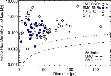
Figure 2: Integrated radio flux densities of SNRs in the LMC (empty symbols) and the SMC (filled symbols), plotted versus SNR diameter. The flux densities of the SMC SNRs have been multiplied by 1.44 for comparison. The circles indicate flux densities at 1.4 GHz, the triangles are at higher frequencies (see Table 1 for details). The dashed and dotted lines show conservative $5\sigma$ limits for the selection of candidate SNRs in both galaxies, accounting for the flux limit per beam and the number of beams per object of given diameter (see Hughes et al., 2007; Filipović et al., 2002). The SMC limit has also been scaled by 1.44. There is a real paucity of SNRs below a flux density of $\sim 50$ mJy at 50 kpc, corresponding to a luminosity of $\sim 1.5\times 10^{15}$ W Hz^-1.

The degree of completeness of our sample is hard to estimate, because we include objects that were found using a very hetrogeneous mix of selection criteria, but a number of factors indicate that we should not be missing a large number of SNRs. First, the floor at 50 mJy is much brighter than the nominal sensitivity of the ATCA/Parkes radio surveys, which at 1.4 GHz is around 0.3 mJy per beam in the LMC (Hughes et al., 2007), and 1.8 mJy per beam in the SMC (Filipović et al., 2002), with beam sizes of $40^{\prime\prime}$ and $98^{\prime\prime}$, respectively. Even requiring at least a $5\sigma$ detection for the selection of SNR candidates, and allowing for the fact that large SNRs should be harder to identify at the same level of significance, the vast majority of our objects are safely above any conservative detection limits in the radio (see Figure 2). Second, the systematic searches for SNRs on the ATCA/Parkes surveys by Filipović et al. (2005) and Payne et al. (2008) have not uncovered a substantial population of previously unknown SNRs between the radio floor and the detection limits. We note that the total number of confirmed SNRs reported (but not listed) by Payne et al. (2008) in the LMC is very close to our own count (52 vs. 54). Third, the existence of a substantial population of radio detected SNRs that are masquerading as other kinds of sources is unlikely in the presence high quality multi-wavelength data. Small, radio-faint SNRs that might be mistaken for background sources are often young objects with bright X-ray emission like SNRs J0509.5$-$6731 (B0509$-$67.5) or J0505.7$-$6753 (DEM L71). Older, more extended objects that might be confused with surrounding or nearby HII regions are usually identified at optical wavelengths by diagnostic quantities like the [S II]/H$\alpha$ ratio, which can be used to distinguish shocked nebulae from photoionized gas (Fesen et al., 1985).

A related concern is that some SNRs might be “lost” inside superbubbles formed by several nested SN explosions (Mac Low & McCray, 1988). In practice, SNRs evolving inside low-density cavities do not disappear – they just become fainter and evolve more slowly, at least until the blast wave reaches the cavity edges. The largest, most prominent superbubble complex in the LMC, 30 Doradus, harbors several well-studied SNRs, including J0537.8$-$6910 (N157B) (Townsley et al., 2006), and many other objects listed in Table 1 are associated with superbubbles. As long as the surveys are sensitive enough to find faint SNRs, this should not be a major issue.

In the absence of a systematic re-analysis of all the available data with a set of homogeneous criteria to identify SNRs in both Clouds, we cannot guarantee that our sample is $100\%$ complete. Such an analysis is outside the scope of the present work, but all the evidence seems to indicate that our compilation should not be missing a large number of objects, and it should include few, if any, spurious ones. We conclude that our list of MC SNRs is at least fairly complete (which is enough for our goals), and that the paucity of SNRs below $\sim 50$ mJy is probably real, and not due to any observational selection effects. This suggests that any MC SNRs with flux densities between the radio floor and the detection limits must fade relatively quickly. As we shall discuss in § 6, the results of Paper II can be used to argue independently that the SNR sample we have compiled has a high degree of completeness.

3 The distribution of remnant sizes

Figure 3 shows the cumulative and differential histograms of remnant sizes in the LMC and in the SMC. In both Clouds, the cumulative distributions are roughly linear in remnant size, i.e., with an equal number of remnants per equal size bin in the differential distributions, up to a cutoff at a physical radius $r_{\rm cut}\sim 30$ pc.

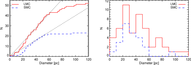
Figure 3: Distribution of the SNR sizes listed in Table 1 for the LMC (red solid plots) and SMC (blue dashed plots), represented as cumulative (left) and differential (right) histograms. For illustrative purposes, linear size distributions normalized to give the correct number of SNRs at a diameter of 40 pc have been overplotted as dotted lines on the cumulative histograms. Both galaxies have SNR size distributions that are close to linear in the cumulative, or flat in the differential, up to a cutoff at $r\sim 30$ pc.

Because the data points in a cumulative histogram are not independent of one another, these curves cannot be fitted in the usual way (using the $\chi^{2}$ statistic). A robust, quantitative estimate for the slope of the distributions can be obtained by performing instead a maximum-likelihood fit, as follows (see Maoz & Rix, 1993, for a similar treatment applied to a different problem). Suppose that a particular model predicts a size distribution $dN/dr=n(r)$, which integrates to $\int_{0}^{r_{\rm cut}}n(r)dr=N$, where $N$ is the total number of remnants up to $r_{\rm cut}$. If we bin our data into many small bins between $r=0$ and $r_{\rm cut}$, each of width $\delta r$, most bins will have zero SNRs, and some will have one SNR. Given the model, the Poisson probability of finding $j$ remnants in the $i$th bin, for which the model predicts $n(r_{i})$ remnants, is

$$P(j|n(r_{i}))=e^{-n(r_{i})}n(r_{i})^{j}/j!.$$ (1)

We will define the likelihood of a given model as the product of these probabilities. The logarithm of the likelihood, considering that $j$ always equals either 0 or 1, simplifies to

$$\ln L=[\sum_{i(j>0)}\ln n(r_{i})]-N,$$ (2)

where the summation is only over the specific data values of the SNR radii. A power law of index $\alpha$, having the proper normalization, will have the form

$$n(r)=\frac{N(\alpha+1)}{r_{\rm cut}^{\alpha+1}}r^{\alpha}.$$ (3)

Inserting in Eq. 2, differentiating $\ln L$ with respect to $\alpha$, and equating to zero to find the maximum gives the maximum likelihood solution,

$$(\alpha+1)_{\rm ml}=\frac{N}{N\ln r_{\rm cut}-\sum_{j>0}\ln r_{i}},$$ (4)

with an uncertainty on $\alpha$ of

$$\Delta\alpha=\left(-\frac{d^{2}(\ln L)}{d\alpha^{2}}\right)^{-1/2}=\frac{\alpha+1}{\sqrt{N}}.$$ (5)

This procedure yields a maximum likelihood index of $\alpha=0.14\pm 0.18$ for the LMC, and $\alpha=0.32\pm 0.28$ for the SMC. Thus, the LMC appears to indeed have a SNR size distribution that is close to uniform. In the SMC, the best fit is intermediate between a flat distribution and one that rises linearly with radius, but given the smaller number of SNRs, it is consistent with both slopes. From Figure 3, it appears that the steeper slope in the SMC is driven by the small-radius side of the distribution. Indeed, if we fit separately the first 8 points and the following 14 points, the maximum likelihood solution is $\alpha=1.7\pm 1.0$ at small radii, and $\alpha=0.17\pm 0.23$ thereafter. This result confirms the visual impression, but formally it is still consistent with a slope close to zero at all radii at the $1.7\sigma$ level. We conclude that the SNR size distribution in both Clouds is consistent with being roughly uniform, although there are hints for a deviation at small radii in the SMC. It is possible that a deficit at small radii is also present in the LMC distribution (see Figure 3), but the Poisson errors are too large to claim that the data require it.

The linear cumulative distribution of SNR sizes in the MCs (and also the Milky Way) has been previously noted and discussed by Mathewson et al. (1984), Mills et al. (1984), Green (1984), Hughes et al. (1984), Fusco-Femiano & Preite-Martinez (1984), Berkhuijsen (1987), Chu & Kennicutt (1988), and most recently by Bandiera & Petruk (2010). Several of these papers also pointed out cutoffs in the distribution. All of these papers considered smaller SNR samples, often based on much shallower radio data and, with few exceptions, did not include multi-wavelength observations. Some of these authors interpreted the observed size distribution as evidence that most MC SNRs are in their “free expansion” phase, during which the shock velocity is constant, and inferred that these SNRs expand into an extremely low-density medium. Alternatively, Green (1984) and Hughes et al. (1984) warned that the observed distribution was the result of selection effects; most objects they discussed had been selected in X-rays, and the X-ray flux limits then led to the exclusion of larger and fainter remnants, and their faint radio counterparts. Our present compilation is bigger, it incorporates the most recent multi-wavelength data, it extends to larger sizes, and most importantly, it is sensitive to radio flux densities two orders of magnitude below the observed luminosity floor. With these data we now confirm the luminosity floor, the uniform size distribution, and the cutoff at $r_{\rm cut}\sim 30$ pc in the Magellanic Cloud SNRs.

These features of the SNR size distribution are also present in other galaxies. Due to its proximity and face-on orientation, M33 has probably the best SNR sample outside of the MCs. The most recent catalogue of M33 SNRs has been published by Long et al. (2010), and it includes data in the radio, optical, and X-rays (from the ChASeM33 survey by Chandra, Plucinsky et al., 2008). The distribution of SNR sizes given in Table 3 of Long et al. (2010), which we plot in Figure 4, has the same broad characteristics we find in the Clouds, but backed by much better statistics (137 objects). The cutoff at a physical radius of $r\sim 30$ pc is very clear, and the distribution appears remarkably uniform for radii between $\sim 10$ pc and the cutoff. In this size range, our method to estimate the maximum likelihood index yields $\alpha=0.04\pm 0.11$. Graphically, a linear function with the correct normalization reproduces the cumulative histogram quite well (see Figure 4). A significant deficit of SNRs at radii below 10 pc is also obvious in the data. Long et al. (2010) warn that a few small (young) SNRs might have escaped detection (see their Section 9), but given the numbers involved, most of the deficit may be real. This indicates a deviation at small diameters from the uniform distribution along the lines of the one we noted in the MCs.

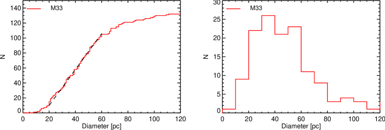
Figure 4: Distribution of SNR sizes in M33 from Long et al. (2010), represented as cumulative (left) and differential (right) histograms. A linear size distribution for diameters between 20 and 60 pc, normalized to give the correct number of SNRs at a diameter of 40 pc, has been overplotted as a dashed line on the cumulative histogram.

The available data seem to indicate that the distribution of SNR sizes in M33 and the Magellanic Clouds is indeed close to uniform between $r\sim 10$ pc and a sharp cutoff at $r_{\rm cut}\sim 30$ pc. In the case of M33, this conclusion needs to be validated by a careful assessment of the completeness of the SNR sample, although from the discussion in § 7.3 of Long et al. (2010) it seems unlikely that a large number of M33 SNRs have escaped detection. Unfortunately, SNR samples of this quality are hard to obtain for other galaxies, so it is difficult to verify how widespread these features of the SNR size distribution are in reality. We will return briefly to this issue in § 7. In the following section, we argue that a uniform size distribution, including a deficit of SNRs at small radii and a sharp cutoff at a certain radius, arises naturally from the physics of SNR evolution and the distribution of densities in the interstellar medium.

4 Physics behind the size distribution

The evolution of SNRs is usually separated into three phases (e.g. Woltjer, 1972). In the first, free-expansion, phase, the mass swept up by the expanding shock is small compared to the ejected mass, and the shock velocity is constant with time. In the Sedov-Taylor phase, the swept-up mass is larger than the ejecta mass, and the expansion decelerates. However, the cooling time of the shocked gas is still longer than the age of the remnant, and the evolution is approximately adiabatic. Once the cooling time becomes comparable to the age, the SNR quickly loses energy radiatively, entering the radiation-loss-dominated snowplough phase, after which it slows down, breaks up, and merges with the interstellar medium.

Quantitative estimates show that typical SNRs should be in their Sedov-Taylor phases for ages between a few and a few tens of kyrs, and for sizes of order a few to a few tens of parsecs (e.g. Cioffi et al., 1988; Blondin et al., 1998; Truelove & McKee, 1999). Thus, most of the MC SNRs in our sample should be in the Sedov-Taylor phase of their expansions, with radii growing as

$$r\sim E_{0}^{1/5}\rho^{-1/5}t^{2/5},$$ (6)

where $E_{0}$ is the kinetic energy of the explosion, $\rho$ is the ambient gas density, and $t$ is the time. The shock velocity therefore decreases as

$$v=\frac{dr}{dt}\sim E_{0}^{1/5}\rho^{-1/5}t^{-3/5},$$ (7)

or equivalently expressed in terms of $r$ rather than $t$,

$$v\sim E_{0}^{1/2}\rho^{-1/2}r^{-3/2}.$$ (8)

Reasonably assuming a constant SN rate in the LMC over the past few kyrs, $dN/dt={\rm const.}$, the naively expected size distribution of SNRs in their Sedov phase is

$$\frac{dN}{dr}=\frac{dN}{dt}\frac{dt}{dr}\sim r^{3/2},$$ (9)

where we have used Eq. 8 to substitute for $dt/dr$. This is contrary to the observed nearly uniform ($dN/dr\sim r^{0}$) distribution. As noted above, this has been interpreted before either as evidence for free expansion, or for selection effects, where fading of the older (and hence larger) remnants takes them below the detection limits, and culls the pileup in the distribution expected at large sizes for a decelerating population. Both explanations are unlikely for our MC SNR sample.

We propose, instead, that the uniform size distribution arises as a result of the transition from the Sedov phase to the radiative phase (see also Fusco-Femiano & Preite-Martinez, 1984; Bandiera & Petruk, 2010). The radius of this transition depends on ambient density, with SNRs evolving in dense environments becoming radiative sooner than SNRs in low-density regions. When coupled with the distribution of densities in the Clouds, this leads to fewer and fewer sites at which large-radius Sedov-phase SNRs can exist. We show this as follows.

The cooling time of the shocked gas depends on the density as

$$t_{\rm cool}\sim\frac{kT}{\rho\Lambda(T)}$$ (10)

where $\Lambda(T)$ is the cooling function at temperature $T$. Following, e.g., McKee & Ostriker (1977), Blondin et al. (1998), or Truelove & McKee (1999), $\Lambda(T)$ can be approximated with piecewise power laws, with a dependence of $T^{\epsilon}$ in the temperature range of relevance for the shocked gas, around $10^{6}~{}{\rm K}$. By relating the temperature to the shock velocity $v$, $kT\sim m_{p}v^{2}$ (where $m_{p}$ is the proton mass), and equating $t_{\rm cool}$ to the age $t$ as expressed in Eq. 7, one obtains that the transition radius, $r_{\max}$, scales as (e.g. Bandiera & Petruk, 2010)

$$r_{\rm max}\sim E_{0}^{(3-2\epsilon)/(11-6\epsilon)}\rho^{-(5-2\epsilon)/(11-6\epsilon)}.$$ (11)

A remnant expanding beyond this radius, at the given ambient density, will enter the radiative phase and quickly fade from view. For a fairly large range of plausible cooling function dependences, e.g., indices $\epsilon$ of $-1/2$ to $-3/2$, $r_{\rm max}$ depends on density as $\rho^{-3/7}$ to $\rho^{-2/5}$. Conversely, the maximum ambient density that will permit a Sedov-phase SNR of radius $r$ is

$$\rho_{\rm max}\propto r^{\delta},$$ (12)

where $\delta$ is likely in the range $-7/3$ to $-5/2$.

The expected size distribution of remnants will now be

$$\frac{dN}{dr}=\frac{dN}{dt}\frac{dt}{dr}\sim r^{3/2}\int_{\rho_{\rm min}}^{\rho_{\rm max}}\rho^{1/2}\frac{dP}{d\rho}d\rho,$$ (13)

where $dP/d\rho$ is the distribution of gas densities in a given galaxy, and ${\rho_{\rm min}}$ is the minimum density in that galaxy, on the size scales relevant for SNRs. Let us parametrize the density distribution as a power law of index $\beta$,

$$\frac{dP}{d\rho}\sim\rho^{\beta},$$ (14)

with $\beta>-3/2$. Then, substituting in Eq. 13, integrating, and expressing $\rho_{\rm max}$ in terms of $r$ using Eq. 12, gives a remnant size distribution

$$\frac{dN}{dr}\sim r^{\delta(\beta+3/2)+3/2}.$$ (15)

A uniform size distribution, $dN/dr\approx{\rm const.}$, is obtained if $\beta=-6/7$ (for $\delta=-7/3$) or $\beta=-9/10$ (for $\delta=-5/2$). In other words, the observed, roughly uniform, SNR size distribution implies a powerlaw distribution of densities with index $\beta\approx-1$.

We note that, because of the dependence of $r_{\rm max}$ on $t_{\rm cool}$, $r_{\rm max}$ can depend on the metallicity of the gas, $Z$. Assuming a cooling function proportional to $Z$, Eq. 11, in addition to the dependence on $\rho$ and $E_{0}$, will depend on $Z$ as

$$r_{\rm max}\sim Z^{-2/(11-6\epsilon)}.$$ (16)

However, in dwarf galaxies like the MCs, where $Z$ does not change much from one location to another, this will be a small effect. For example, if $\epsilon=-1$, changing $Z$ by a factor 5 would only change $r_{\rm max}$ by $\sim 20\%$.

The existence of a cutoff in the distribution beyond some size is naturally expected in the above picture, given the existence of some minimum density $\rho_{\rm min}$ in the regions of the galaxies where SNe explode, and in view of the decrease of $\rho_{\rm max}$ with radius. At some radius, $\rho_{\rm max}$ will equal $\rho_{\rm min}$ and the integral in Eq. 13 will therefore become zero. In other words, there will be nowhere in the MCs a region with a density low enough to permit a SNR of that size that is still in its bright Sedov phase.

A deficit of SNRs at small radii, as observed in M33 and the MCs, is also expected in this scenario. Before the onset of the Sedov stage, faster shock velocities will lead to fewer objects observed in the bins with the smallest radii. This onset happens at ages (sizes) that depend on the details of the ejecta structure, as well as the ambient density (see § 7 in Truelove & McKee, 1999), but for most SNRs it should occur around a few hundred years (a few pc), which is consistent with the deficits that we have observed in M33 and the MCs. This regime affects only a small number of objects in the MCs, and does not impact any of the arguments made above, so we will ignore it for the remainder of the paper.

We have also ignored the deviations from the standard evolutionary picture that can be introduced by the shape of the circumstellar medium excavated by the SN progenitors. Badenes et al. (2007) showed that most Type Ia SNRs with known ages have sizes that are consistent with an interaction with a uniform ambient medium, but no such study has been done for CC SNRs. The fast stellar outflows expected from the more massive CC SN progenitors will modify the sizes of a few individual SNRs at certain stages of their evolution (e.g., Dwarkadas, 2005, 2007), but most of the objects that we consider here are too large to be expanding in even the most extreme wind-blown cavities. As long as the bulk of the SNRs in the sample spend most of their lifetimes in the Sedov stage, this should not affect our scenario. Similarly, the fact that some SNRs evolve inside superbubbles (e.g. Mac Low & McCray, 1988) is naturally incorporated into our picture – superbubbles merely become one more of the factors driving the density distribution in the interstellar medium. Incidentally, the size distribution of superbubbles also relates to the properties of the interstellar medium, as shown by Oey & Clarke (1997) for several nearby galaxies, including the SMC.

5 Three estimates of the gas density distribution in the Magellanic Clouds

As we have seen, a uniform SNR size distribution can be understood as the result of Sedov expansion, combined with a transition to the radiative phase at an age that depends on the local density, provided that the density of the gas in the interstellar medium follows a distribution close to a power law with an index of $-1$, $dP/d\rho\sim\rho^{-1}$. In this Section, we test this hypothesis by examining three indirect tracers of gas density in the Magellanic Clouds: HI column density; star-formation rate (SFR) based on resolved stellar populations; and H$\alpha$ emission-line surface brightness. These tracers are well suited for our goals because they are valid over a wide range of densities, and the necessary data are available from public surveys that cover the whole extent of the Clouds, as described in detail below.

5.1 21 cm emission-line-based HI column density

We have taken the surface brightness of HI 21 cm line emission in the MCs from the maps of Kim et al. (2003) and Stanimirovic et al. (1999), which combine single-dish Parkes and aperture-synthesis ATCA data to probe both small and large scales in the LMC and the SMC, respectively. The 21 cm emission is optically thin, so the surface brightness is directly proportional to the HI column density. Since the LMC possesses a fairly face-on (inclination $i\sim 35^{\circ}$, van der Marel & Cioni, 2001), well-ordered HI disk, the column density should, in turn, be roughly proportional to the volume density $\rho$. Kim et al. (2007) report that the HI column density distribution of individual “clouds” of neutral hydrogen in the LMC follows a log-normal form, rather than a power law. However, their figure 13 suggests that, above a low cutoff of $2\times 10^{20}~{}{\rm cm}^{-2}$, the distribution does behave as a power law of slope $\sim-1$, over at least an order of magnitude. To re-examine this, in Figure 5 we show the differential distribution of HI column density in the individual beam-sized pixels of the Kim et al. (2003) LMC map (as opposed to the cumulative plot for “clouds” shown in Kim et al., 2007). We see that the HI column in the LMC does follow an index $-1$ power law fairly well, between a column of $3\times 10^{20}~{}{\rm cm}^{-2}$ and $6\times 10^{21}~{}{\rm cm}^{-2}$. The observed low cutoff in the column density is unavoidable because of the integration through the disk and over the beam size (every line of sight is basically sampling the densest regions at that point). In regions with low density, the H atoms might be ionized, as in the “warm ionized” phase of the interstellar medium (Ferrière, 2001), so the tracer may become less reliable there. It is quite plausible that, in the regions where SNe actually explode, the underlying distribution of densities also reaches a minimum – as we recall, a minimum density is required in order to reproduce the observed upper cutoff in SNR size – but this does not necessarily correspond with the lower threshold in the HI distribution. To illustrate this, we have calculated the mean HI columns in each of the spatial “cells” defined by Harris & Zaritsky (2004) and Harris & Zaritsky (2009) that contain SNRs (see § 5.2 below for a description of the cells), which we display with the horizontal rulers in Figure 5. We note that, in the LMC, these cells have average column values between $5\times 10^{20}~{}{\rm cm}^{-2}$ (close to, but higher than the low HI cutoff) and $6\times 10^{21}~{}{\rm cm}^{-2}$, although most SNRs appear clustered around $2\times 10^{21}~{}{\rm cm}^{-2}$.

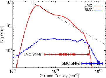
Figure 5: Binned histogram of neutral H column densities in the LMC (red) and the SMC (blue). The dotted line overlaid on the LMC histogram is a power law of index $-1$ that intersect the data at a column of $5\times 10^{20}\,\rm{cm^{-2}}$. The column density values for the cells that contain the SNRs in both galaxies have been represented by tick marks on the horizontal rulers.

As shown in Figure 5, the distribution of HI column densities in the SMC is flat over the same range, although the rise and fall from the plateau happen at the same densities as the rise and fall of the powerlaw in the LMC. While we do not know the reason for this, we speculate that it may be related to an SMC geometry that is elongated along our line of sight, and the integration effect that results. The actual “depth” of the SMC, whether just a few kpc or as much as 20 kpc, is debated (Hatzidimitriou & Hawkins, 1989; Harris & Zaritsky, 2004; Subramanian & Subramaniam, 2009), but is likely at least a few times larger than that of the nearly face-on LMC. Such an integration effect would explain why the SMC SNRs are found at HI column densities that are a factor $\sim$4 higher than the LMC SNRs (see horizontal rulers in Figure 5). Two other tracers of density, examined below, do suggest a $-1$ power law in the SMC, as well as in the LMC, and do not display this offset in SNR ambient densities.

5.2 Schmidt Law plus star formation rates from resolved stellar populations

As a second way to estimate the local gas densities and test the powerlaw density distribution hypothesis, we use star formation rates (SFRs) calculated from the star-formation history (SFH) maps of the MCs published by Harris & Zaritsky (2004) and Harris & Zaritsky (2009), which are based on resolved stellar populations. The maps were elaborated using four-band (U, B, V, and I) photometry from the Magellanic Clouds Photometric Survey (Zaritsky et al., 2004), which has a limiting magnitude between 20 and 21 in V, depending on the local degree of crowding in the images. In each Cloud, the data were divided into regions or “cells” with enough stars to produce color-magnitude diagrams of sufficient quality, which were then fed into the StarFISH code (Harris & Zaritsky, 2001) to derive the local SFH for each cell. For the LMC, Harris & Zaritsky (2009) divided more than 20 million stars into spatial cells encompassing the central 8${}^{\circ}\times 8^{\circ}$ of the galaxy (see their figure 4). In total, they produced 1376 cells for the LMC, most of them $12^{\prime}\times 12^{\prime}$ in size, and about 50 cells in regions of lower stellar density with a larger size ($24^{\prime}\times 24^{\prime}$). For the SMC, Harris & Zaritsky (2004) divided over 6 million stars into 351 $12^{\prime}\times 12^{\prime}$ cells, leaving out two areas that are contaminated by Galactic globular clusters in the foreground (see their figure 3).

Harris & Zaritsky (2004) and Harris & Zaritsky (2009) provide the SFH for each of these cells, which we use in Paper II to derive the delay time distribution of SNe in the Clouds, but for our present purposes we are only interested in the current SFR, which we have obtained by averaging the star formation in each cell over the last 35 Myr. The Schmidt (1959) law relates star formation to gas mass column, $\Sigma$, roughly as ${\rm SFR}\propto\Sigma^{3/2}$. If gas density is distributed as $\rho^{\beta}$, and $\Sigma\propto\rho$, then SFR will be distributed as a power law of index $2(\beta-1/2)/3$. Coincidentally, if $\beta=-1$, the SFR distribution will also have an index $-1$ powerlaw distribution. Kennicutt (1998) gives an update of the Schmidt law, relating star formation rate surface density, $\Sigma_{\rm SFR}$, to gas mass column $\Sigma_{\rm gas}$, as

$$\Sigma_{\rm SFR}=(2.5\pm 0.7)\times 10^{-4}\left(\frac{\Sigma_{\rm gas}}{M_{\odot}~{}{\rm pc}^{-2}}\right)^{1.4\pm 0.15}M_{\odot}~{}{\rm yr}^{-1}{\rm kpc}^{-2}.$$ (17)

As emphasized by Kennicutt (1989), the Schmidt law has a threshold at a given mass column, below which the star-formation rate falls steeply. The exact value of this threshold is disputed: Kennicutt (1989) finds $\Sigma_{\rm gas}=3-4~{}{\rm M_{\odot}\,pc}^{-2}$, which corresponds to $\sim 1.4\times 10^{-3}~{}{\rm M_{\odot}\,yr^{-1}\,kpc}^{-2}$, but higher and lower threshold values have also been reported in the literature (see Bigiel et al., 2008, for an updated discussion of this issue). From Eq. 17 with $\Sigma_{\rm gas}=3.5~{}M_{\odot}{\rm pc}^{-2}$, the threshold mass column corresponds to a SFR of $0.0014~{}M_{\odot}~{}{\rm yr}^{-1}{\rm kpc}^{-2}$, or $4.3\times 10^{-5}~{}M_{\odot}~{}{\rm yr}^{-1}$ per $12^{\prime}\times 12^{\prime}$ cell in the Harris & Zaritsky (2009) maps of the LMC.

Figure 6 shows that, above a value of $\sim(2-4)\times 10^{-4}M_{\odot}~{}{\rm yr}^{-1}~{}{\rm cell}^{-1}$, the SFR is indeed distributed as a power law of index $-1$, over more than one order of magnitude in SFR, for both the LMC and the SMC. To meaningfully compare the SFRs in cells with different physical areas, we have counted the few $24^{\prime}\times 24^{\prime}$ cells in the LMC as four $12^{\prime}\times 12^{\prime}$ cells with the same SFR, and we have scaled down the SFRs of all the $12^{\prime}\times 12^{\prime}$ cells in the SMC by a factor of 1.44, to account for the fact that this galaxy is 20% more distant than the LMC.

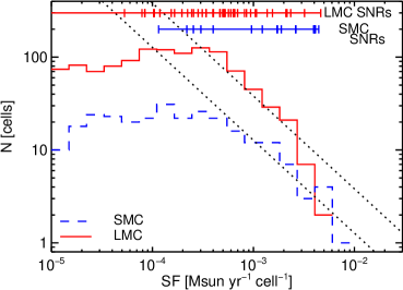
Figure 6: Binned histogram of star formation rates averaged over the last 35 Myr in the LMC (red, solid plot) and the SMC (blue, dashed plot). The dotted lines are power laws of index $-1$ that intersect the data at a SFR of $2\times 10^{-3}\,\rm{M_{\odot}\,yr^{-1}\,cell^{-1}}$. The SFR values for the cells that contain the SNRs in both galaxies are represented by tick marks on the horizontal rulers.

5.3 Schmidt Law plus star formation rates from H$\alpha$ emission

Rather than measuring SFR via the resolved stellar populations of the MCs, we can trace it by means of H$\alpha$ emission, which gives us a third probe of gas density. H$\alpha$ is principally powered by photoionisation from O-type stars, whose numbers are proportional to the SFR. The Schmidt law again connects this SFR to the gas mass column. We have examined the continuum-subtracted H$\alpha$ emission maps of the LMC and SMC from the SHASSA survey of Gaustad et al. (2001) . Figure 7 shows that both the LMC and the SMC have distributions of H$\alpha$ surface brightness that follow power laws of index $\sim-1$, this time over 2 orders of magnitude for the SMC, and almost 3 for the LMC. As before, through the Schmidt law, this implies a power law with index $-1$ for the gas density distribution over 1-2 orders of magnitude in density. Surface brightness is independent of distance for such nearby galaxies, and can therefore be compared directly between the LMC and SMC.

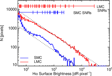
Figure 7: Binned histogram of H$\alpha$ surface brightness in the LMC (red) and the SMC (blue). Dotted lines are power laws of index $-1$ that intersects the data at $2\times 10^{3}$ dR pixel^-1. The flux values for the cells that contain the SNRs in both galaxies are represented by tick marks on the horizontal rulers.

5.4 The Interstellar Medium of the Magellanic Clouds

The density tracers that we have examined here are not free of biases, but they should provide a fairly accurate picture of the density distribution in the interstellar medium of the MCs. Specific regions within the Clouds, like the LMC bar or 30 Dor, will probably have density distributions that are different from the simple powerlaws we have found here; our analysis only applies to the bulk, statistical properties of the gas on galactic scales. Several theoretical studies have adressed the probability distribution of densities in the interstellar medium: see Padoan et al. (1997), Passot & Vázquez-Semadeni (1998), Scalo et al. (1998), and Wada & Norman (2001). The consensus of these studies is that, despite local inhomogeneities and deviations, a combination of galaxy-wide and local mechanisms conspire to produce a lognormal distribution of densities in the gas for a wide range of conditions. At the higher densities where most stars are formed and most SNe explode, the tail of the lognormal distribution is well reproduced by a power law with an index $\sim-1$ (see figure 19 in Wada & Norman, 2007). This is consistent with our findings for the MCs.

6 Discussion

The derivation in § 4 ignores many subtleties in what is clearly a complex problem, involving different physical processes and temporal scales. In this context, the fact that the distribution of gas densities in the MCs seems to behave like a power law with an index $\sim-1$ does not prove that our proposed picture for the evolution of SNRs is correct. However, our simple (but physically motivated) scenario appears to explain the available observations quite well, and is consistent with what we know about the bulk properties of the interstellar gas in the MCs. Furthermore, there are indirect ways to test that the basic scenario is sound.

In Paper II, we use the compilation of SNR observations from Table 1 and the SFH maps of Harris & Zaritsky (2004) and Harris & Zaritsky (2009) to derive the SN rate and delay time distribution in the Magellanic Clouds. Some key results from that exercise, which we describe briefly here, serve as plausibility arguments for our picture of SNR evolution. A basic ingredient in the derivation of SN rates is the “visibility time” of SNRs (i.e., the time during which a SNR would be visible, if it were there). We have identified this time with the transition to the radiative phase in § 4, but without assigning any specific value to it. This cannot be done using theoretical arguments alone, because many of the necessary parameters are not known with sufficient accuracy, like the distribution of SN kinetic energies or the normalization of the cooling function (see Eq. 11). The visibility time cannot be calibrated using individual objects either, because the only SNRs that have reliable ages from light echoes or historical observations are much younger than the old SNRs in the Sedov stage that form the bulk of our sample.

In Paper II, this conundrum is solved by imposing a condition on the delay time distribution: that the vast majority of stars more massive than $8\,\mathrm{M_{\odot}}$ explode as core collapse SNe, with very few “silent” events that collapse directly to form a black hole without much ejection of material and hence without leaving a SNR behind. If this condition holds, an absolute value for the SNR visibility time can be obtained by equating the time-integrated SN rate in the temporal bin of the delay time distribution that is associated with core collapse SNe (in the binning used in Paper II, that is all SNe with delays shorter than 35 Myr) to the number of massive stars per total stellar mass formed. This procedure yields SNR visibility times that depend on the tracer used to determine the local density, and vary between $13.3$ kyr (for the HI density tracer) and $22.5$ kyr (for the SFR-based density tracer – see table 2 in Paper II). These ages are for regions where the local density corresponds to the mean value of the tracer, $1.5\times 10^{21}~{}{\rm cm}^{-2}$ and $3.3\times 10^{-4}~{}M_{\odot}~{}{\rm yr}^{-1}\,\mathrm{cell}^{-1}$, respectively (see Figures 5 and 6); for values 10 times lower than the mean, the visibility times could be a factor 3 to 4 longer (see Paper II for details). This is in good agreement with the maximum ages of SNR shells inferred by SNR-pulsar associations in the Milky Way, which are $\sim 60$ kyr (Frail et al., 1994; Gaensler & Johnston, 1995).

Another key result from Paper II is the total rate of SNe (CC and Type Ia) in the Magellanic Clouds. The rate depends again on the density tracer used to estimate the visibility time, and varies between $4.1\pm 0.9\times 10^{-3}\,\mathrm{SN\,yr^{-1}}$ (for HI) and $2.4\pm 0.4\times 10^{-3}\,\mathrm{SN\,yr^{-1}}$ (using SFR as the tracer). These rates, and the visibility times quoted in the previous paragraph, are derived assuming that our SNR sample is complete and our evolution scenario is correct. As explained in Paper II, the rates, when normalized per unit stellar mass, are typical of dwarf irregular galaxies, of which the MCs are prototypes. The rates are also in loose agreement with the historical records, which show 2 SNe in the MCs in the last 400 yr (i.e., roughly $5\times 10^{-3}\,\mathrm{SN\,yr^{-1}}$, see discussion in § 5.3 of Badenes et al., 2008), although this number of events is too small to put strong constraints on the SN rate. Adopting the assumption that most SNRs are actually in free expansion and not in the Sedov stage, as has been invoked by a number of authors to explain the observed uniform size distribution (see § 3), would lead to inconsistencies. Undecelerated SN ejecta reach velocities in excess of 10000 km s^-1, so we would expect the shock velocities in freely expanding SNRs to be in the range $\sim 5000$ to 10000 km s^-1. At these velocities, the cutoff radius of $r\sim 30$ pc would translate to maximum ages of 3 to 6 kyr. The 77 SNRs in the MCs would then imply a SN explosion in the MCs once every 40 to 80 years, on average, or even more frequently if our SNR sample is incomplete. Finally, if the visibility time were fixed at 6 kyr, for instance, this would correspond to a CC-SN yield (i.e., the number of CC SNe per stellar mass formed) of $0.022~{}\mathrm{M_{\odot}^{-1}}$ (see Paper II). To produce so many CC-SNe all stars with initial mass above $3.7~{}\mathrm{M_{\odot}}$ in a standard IMF would have to explode, which is in direct contradiction to stellar evolution theory, and to the semi-empirical initial-final mass relation for WDs (Catalán et al., 2008; Salaris et al., 2009; Williams et al., 2009).

7 Summary and Conclusions

In this paper, we have proposed a physically motivated scenario for the evolution of SNRs in the interstellar medium of galaxies, and we have applied it to the sample of SNRs in the Magellanic Clouds. We compiled multi-wavelength observations of the 77 known SNRs in the MCs from the existing literature (Table 1 and Figure 1). We verified that this compilation is fairly complete, and that the size distribution of SNRs is approximately flat, within the allowed uncertainties, up to a cutoff at $r\sim 30$ pc, as discussed by other authors before. We noted that these features are also present in the larger SNR sample assembled by Long et al. (2010) for M33. In our model, the flat size distribution can be explained if most SNRs are in the Sedov, decelerating, stage of their expansion, quickly fading below detection as soon as they reach the radiative stage at an age (size) that depends on the local density. Under these circumstances, a flat distribution of SNR sizes arises naturally if the probability distribution of densities in the gas follows a power law with index $-1$. To test this hypothesis, we have examined the distributions of three different density tracers in the Clouds: HI column density, H$\alpha$ flux, and SFR obtained from resolved stellar populations. We have verified that these tracers do indeed indicate a density distribution that follows a power law with index $-1$, over a wide range of densities, and that this agrees with our theoretical understanding of the dynamics of the interstellar medium. Our scenario implies that SNRs will remain visible for different times at different locations in the Magellanic Clouds, depending on the local density. This visibility time is a key ingredient in the calculation of SN rates and SN delay time distributions, which we derive for the Magellanic Clouds in Paper II. The absolute value of the visibility time cannot be determined from theoretical arguments alone, but we have used the results from Paper II to verify that the range of values we obtain ($13$ to $23$ kyr for regions of mean density, depending on the tracer) is consistent with the existing limits for the maximum ages of SNRs, and with basic stellar evolution theory.

It would be interesting to extend our analysis of SNR sizes and interstellar medium densities to other galaxies in the Local Group. On the one hand, this would allow us to test the validity of our SNR evolution scenario in different settings. On the other hand, the techniques developed here and in Paper II would yield more accurate SN rates and more detailed delay time distributions with larger SNR samples, provided the SFHs in the host galaxies could be determined with enough spatial and temporal resolution. A growing number of nearby galaxies have published SNR catalogues, but samples of the quality of the one we have assembled here for the Magellanic Clouds or the one published by Long et al. (2010) for M33 are hard to obtain. Interstellar extinction and distance uncertainties plague the Milky Way SNRs, and the radio detection limits become comparable to the fluxes of the fainter Magellanic Cloud SNRs for distances beyond several hundred kpc (see Chomiuk & Wilcots, 2009). With a judicious investment of observing time, however, reasonably complete multi-wavelength catalogues of SNRs in a few well-suited nearby galaxies could become available in the near future.

References

- Alves (2004) Alves D. R., 2004, New Astronomy Review, 48, 659
- Badenes (2010) Badenes C., 2010, Proceedings of the National Academy of Science, 107, 7141
- Badenes et al. (2009) Badenes C., Harris J., Zaritsky D., Prieto J. L., 2009, ApJ, 700, 727
- Badenes et al. (2007) Badenes C., Hughes J. P., Bravo E., Langer N., 2007, ApJ, 662, 472
- Badenes et al. (2008) Badenes C., Hughes J. P., Cassam-Chenaï G., Bravo E., 2008, ApJ, 680, 1149
- Bamba et al. (2006) Bamba A., Ueno M., Nakajima H., Mori K., Koyama K., 2006, A&A, 450, 585
- Bandiera & Petruk (2010) Bandiera R., Petruk O., 2010, A&A, 509, A34+
- Berkhuijsen (1987) Berkhuijsen E. M., 1987, A&A, 181, 398
- Bigiel et al. (2008) Bigiel F., Leroy A., Walter F., Brinks E., de Blok W. J. G., Madore B., Thornley M. D., 2008, AJ, 136, 2846
- Blondin et al. (1998) Blondin J. M., Wright E. B., Borkowski K. J., Reynolds S. P., 1998, ApJ, 500, 342
- Bojičić et al. (2007) Bojičić I. S., Filipović M. D., Parker Q. A., Payne J. L., Jones P. A., Reid W., Kawamura A., Fukui Y., 2007, MNRAS, 378, 1237
- Borkowski et al. (2006) Borkowski K. J., Hendrick S. P., Reynolds S. P., 2006, ApJ, 652, 1259
- Catalán et al. (2008) Catalán S., Isern J., García-Berro E., Ribas I., 2008, MNRAS, 387, 1693
- Chen et al. (2006) Chen Y., Wang Q. D., Gotthelf E. V., Jiang B., Chu Y., Gruendl R., 2006, ApJ, 651, 237
- Chevalier (1982) Chevalier R., 1982, ApJ, 258, 790
- Chomiuk & Wilcots (2009) Chomiuk L., Wilcots E. M., 2009, ApJ, 703, 370
- Chu & Kennicutt (1988) Chu Y.-H., Kennicutt Jr. R. C., 1988, AJ, 96, 1874
- Cioffi et al. (1988) Cioffi D. F., McKee C. F., Bertschinger E., 1988, ApJ, 334, 252
- Cox (2005) Cox D. P., 2005, ARA&A, 43, 337
- Dopita et al. (2010) Dopita M. A., et al., 2010, ApJ, 710, 964
- Dwarkadas (2005) Dwarkadas V. V., 2005, ApJ, 630, 892
- Dwarkadas (2007) —, 2007, ApJ, 667, 226
- Ferrière (2001) Ferrière K. M., 2001, Rev. Mod. Phys., 73, 1031
- Fesen et al. (1985) Fesen R. A., Blair W. P., Kirshner R. P., 1985, ApJ, 292, 29
- Filipović et al. (2002) Filipović M. D., Bohlsen T., Reid W., Staveley-Smith L., Jones P. A., Nohejl K., Goldstein G., 2002, MNRAS, 335, 1085
- Filipovic et al. (1998) Filipovic M. D., Haynes R. F., White G. L., Jones P. A., 1998, A&AS, 130, 421
- Filipovic et al. (1995) Filipovic M. D., Haynes R. F., White G. L., Jones P. A., Klein U., Wielebinski R., 1995, A&AS, 111, 311
- Filipović et al. (2005) Filipović M. D., Payne J. L., Reid W., Danforth C. W., Staveley-Smith L., Jones P. A., White G. L., 2005, MNRAS, 364, 217
- Frail et al. (1994) Frail D. A., Goss W. M., Whiteoak J. B. Z., 1994, ApJ, 437, 781
- Fusco-Femiano & Preite-Martinez (1984) Fusco-Femiano R., Preite-Martinez A., 1984, ApJ, 281, 593
- Gaensler et al. (2003) Gaensler B. M., Hendrick S. P., Reynolds S. P., Borkowski K. J., 2003, ApJ, 594, L111
- Gaensler & Johnston (1995) Gaensler B. M., Johnston S., 1995, MNRAS, 277, 1243
- Gaetz et al. (2000) Gaetz T. J., Butt Y. M., Edgar R. J., Eriksen K. A., Plucinsky P. P., Schlegel E. M., Smith R. K., 2000, ApJ, 534, L47
- Gaustad et al. (2001) Gaustad J. E., McCullough P. R., Rosing W., Van Buren D., 2001, PASP, 113, 1326
- Green (1984) Green D. A., 1984, MNRAS, 209, 449
- Harris & Zaritsky (2001) Harris J., Zaritsky D., 2001, ApJS, 136, 25
- Harris & Zaritsky (2004) —, 2004, AJ, 127, 1531
- Harris & Zaritsky (2009) —, 2009, AJ, 138, 1243
- Hatzidimitriou & Hawkins (1989) Hatzidimitriou D., Hawkins M. R. S., 1989, MNRAS, 241, 667
- Hendrick et al. (2003) Hendrick S., Borkowski K., Reynolds S. P., 2003, ApJ, 593, 370
- Hendrick et al. (2005) Hendrick S. P., Reynolds S. P., Borkowski K. J., 2005, ApJ, 622, L117
- Hilditch et al. (2005) Hilditch R. W., Howarth I. D., Harries T. J., 2005, MNRAS, 357, 304
- Hughes et al. (2007) Hughes A., Staveley-Smith L., Kim S., Wolleben M., Filipović M., 2007, MNRAS, 382, 543
- Hughes et al. (1984) Hughes J. P., Helfand D. J., Kahn S. M., 1984, ApJ, 281, L25
- Hughes et al. (2006) Hughes J. P., Rafelski M., Warren J. S., Rakowski C., Slane P., Burrows D., Nousek J., 2006, ApJ, 645, L117
- Hwang et al. (2001) Hwang U., Petre R., Holt S. S., Szymkowiak A. E., 2001, ApJ, 560, 742
- Kennicutt (1989) Kennicutt Jr. R. C., 1989, ApJ, 344, 685
- Kennicutt (1998) —, 1998, ARA&A, 36, 189
- Kim et al. (1998) Kim S., Chu Y., Staveley-Smith L., Smith R. C., 1998, ApJ, 503, 729
- Kim et al. (2007) Kim S., Rosolowsky E., Lee Y., Kim Y., Jung Y. C., Dopita M. A., Elmegreen B. G., Freeman K. C., Sault R. J., Kesteven M., McConnell D., Chu Y., 2007, ApJS, 171, 419
- Kim et al. (2003) Kim S., Staveley-Smith L., Dopita M. A., Sault R. J., Freeman K. C., Lee Y., Chu Y., 2003, ApJS, 148, 473
- Long et al. (2010) Long K. S., et al., 2010, ApJS, 187, 495
- Mac Low & McCray (1988) Mac Low M., McCray R., 1988, ApJ, 324, 776
- Magnier et al. (1997) Magnier E. A., Primini F. A., Prins S., van Paradijs J., Lewin W. H. G., 1997, ApJ, 490, 649
- Maoz & Rix (1993) Maoz D., Rix H., 1993, ApJ, 416, 425
- Mathewson et al. (1984) Mathewson D., Ford V., Dopita M., Tuohy I., Mills B., Turtle A., 1984, ApJS, 55, 189
- McKee & Ostriker (1977) McKee C. F., Ostriker J. P., 1977, ApJ, 218, 148
- Mills et al. (1984) Mills B. Y., Turtle A. J., Little A. G., Durdin J. M., 1984, Australian Journal of Physics, 37, 321
- Murphy Williams et al. (2010) Murphy Williams, R. N., Dickel, J. R., Chu, Y., Points, S., Winkler, F., Johnson, M., & Lodder, K. 2010, Bulletin of the American Astronomical Society, 41, 470
- Ng et al. (2008) Ng C.-Y., Gaensler B. M., Staveley-Smith L., Manchester R. N., Kesteven M. J., Ball L., Tzioumis A. K., 2008, ApJ, 684, 481
- Oey & Clarke (1997) Oey M. S., Clarke C. J., 1997, MNRAS, 289, 570
- Padoan et al. (1997) Padoan P., Nordlund A., Jones B. J. T., 1997, MNRAS, 288, 145
- Park et al. (2003a) Park S., Burrows D. N., Garmire G. P., Nousek J. A., Hughes J. P., Williams R. M., 2003a, ApJ, 586, 210
- Park et al. (2003b) Park S., Hughes J. P., Burrows D. N., Slane P. O., Nousek J. A., Garmire G. P., 2003b, ApJ, 598, L95
- Park et al. (2003c) Park S., Hughes J. P., Slane P. O., Burrows D. N., Warren J. S., Garmire G. P., Nousek J. A., 2003c, ApJ, 592, L41
- Passot & Vázquez-Semadeni (1998) Passot T., Vázquez-Semadeni E., 1998, Phys. Rev. E, 58, 4501
- Payne et al. (2008) Payne J. L., White G. L., Filipović M. D., 2008, MNRAS, 383, 1175
- Plucinsky et al. (2008) Plucinsky P. P., et al., 2008, ApJS, 174, 366
- Rakowski et al. (2006) Rakowski C. E., Badenes C., Gaensler B. M., Gelfand J. D., Hughes J. P., Slane P. O., 2006, ApJ, 646, 982
- Reyes-Iturbide et al. (2008) Reyes-Iturbide J., Rosado M., Velázquez P. F., 2008, AJ, 136, 2011
- Salaris et al. (2009) Salaris M., Serenelli A., Weiss A., Miller Bertolami M., 2009, ApJ, 692, 1013
- Scalo et al. (1998) Scalo J., Vazquez-Semadeni E., Chappell D., Passot T., 1998, ApJ, 504, 835
- Schmidt (1959) Schmidt M., 1959, ApJ, 129, 243
- Seward et al. (2006) Seward F. D., Williams R. M., Chu Y., Dickel J. R., Smith R. C., Points S. D., 2006, ApJ, 640, 327
- Smith et al. (2000) Smith C., Leiton R., Pizarro S., 2000, in Astronomical Society of the Pacific Conference Series, Vol. 221, Stars, Gas and Dust in Galaxies: Exploring the Links, D. Alloin, K. Olsen, & G. Galaz, ed., pp. 83–+
- Stanimirovic et al. (1999) Stanimirovic S., Staveley-Smith L., Dickey J. M., Sault R. J., Snowden S. L., 1999, MNRAS, 302, 417
- Subramanian & Subramaniam (2009) Subramanian S., Subramaniam A., 2009, A&A, 496, 399
- Townsley et al. (2006) Townsley L. K., Broos P. S., Feigelson E. D., Brandl B. R., Chu Y., Garmire G. P., Pavlov G. G., 2006, AJ, 131, 2140
- Truelove & McKee (1999) Truelove J., McKee C., 1999, ApJS, 120, 299
- van der Heyden et al. (2004) van der Heyden K., Bleeker J., Kaastra J., 2004, A&A, 421, 1031
- van der Marel & Cioni (2001) van der Marel R. P., Cioni M., 2001, AJ, 122, 1807
- Wada & Norman (2001) Wada K., Norman C. A., 2001, ApJ, 547, 172
- Wada & Norman (2007) —, 2007, ApJ, 660, 276
- Warren et al. (2003) Warren J. S., Hughes J. P., Slane P. O., 2003, ApJ, 583, 260
- Williams et al. (2009) Williams K. A., Bolte M., Koester D., 2009, ApJ, 693, 355
- Williams & Chu (2005) Williams R. M., Chu Y., 2005, ApJ, 635, 1077
- Williams et al. (1999) Williams R. M., Chu Y.-H., Dickel J. R., Petre R., Smith R. C., Tavarez M., 1999, ApJS, 123, 467
- Williams et al. (2000) Williams R. M., Petre R., Chu Y., Chen C., 2000, ApJ, 536, L27
- Woltjer (1972) Woltjer L., 1972, ARA&A, 10, 129
- Zaritsky et al. (2004) Zaritsky D., Harris J., Thompson I. B., Grebel E. K., 2004, AJ, 128, 1606