Parametrization of projector-based witnesses for bipartite systems

Abstract

Entanglement witnesses are nonpositive Hermitian operators which can detect the presence of entanglement. In this paper, we provide a general parametrization for orthonormal basis of ${\mathbb{C}}^{n}$ and use it to construct projector-based witness operators for entanglement detection in the vicinity of pure bipartite states. Our method to parameterize entanglement witnesses is operationally simple and could be used for doing symbolic and numerical calculations. As an example we use the method for detecting entanglement between an atom and the single mode of quantized field, described by the Jaynes-Cummings model. We also compare the detection of witnesses with the negativity of the state, and show that in the vicinity of pure stats such constructed witnesses able to detect entanglement of the state.

Keywords: General orthonormal basis; Entanglement witness; Negativity; Jaynes-Cummings model

PACS numbers: 03.65.Ud, 03.67.-a, 42.50.-p

1 Introduction

The interest on quantum entanglement has dramatically increased over the last two decades due to the emerging field of quantum information theory. It turns out that quantum entanglement provides a fundamental potential resource for communication and information processing [1, 2, 3]. A pure quantum state of two or more subsystems is said to be entangled if it is not a product of states of each components. On the other hand, a bipartite mixed state $\rho$ is said to be entangled if it can not be expressed as a convex combination of pure product states [4], otherwise, the state is separable or classically correlated. It is, therefore, of primary importance testing whether a given state is separable or entangled. For systems with dimensions $2\otimes 2$ or $2\otimes 3$, there exists an operationally simple necessary and sufficient condition for separability, the so called Peres-Horodecki criterion [5, 6]. It indicates that a state $\rho$ is separable if and only if the matrix obtained by partially transposing the density matrix $\rho$ is still positive. However, in higher dimensional systems this is only a necessary condition; that is, there exist entangled states whose partial transpose is positive.

Peres-Horodecki criterion for separability leads to a natural computable measure of entanglement, called negativity [7, 8, 9]. Negativity is based on the trace norm of the partial transpose $\rho^{T_{1}}$ of the bipartite mixed state $\rho$, and measures the degree to which $\rho^{T_{1}}$ fails to be positive, i.e. the absolute value of the sum of negative eigenvalues of $\rho^{T_{1}}$

$${\mathcal{N}}(\rho)\equiv\frac{\parallel\rho^{T_{1}}\parallel_{1}-1}{2},$$ (1)

where $\parallel\rho^{T_{1}}\parallel_{1}$ denotes the trace norm of $\rho^{T_{1}}$. Vidal and Werner [9] proved that the negativity ${\mathcal{N}}(\rho)$ is an entanglement monotone and therefore it is a good measure of entanglement.

The most general approach for detecting entanglement is using entanglement witnesses [6, 10, 11, 12, 13]. Entanglement witnesses are operators that are designed directly for distinguishing between separable and entangled states. By definition, we say that a Hermitian operator $W$ defined on the product space ${\mathcal{H}}={\mathcal{H}}_{1}\otimes{\mathcal{H}}_{2}$ is an entanglement witness if and only if: 1) ${\rm Tr}(W\sigma)\geq 0$ for all separable states $\sigma\in{\mathcal{S}}$, and 2) there exists at least one entangled state $\rho$ such that ${\rm Tr}(W\rho)<0$. The negative expectation value is hence a signature of entanglement, and for a state $\rho$ with ${\rm Tr}(W\rho)<0$ we say that it is detected by $W$. It turns out that a state is entangled if and only if it is detected by some entanglement witnesses $W$ [6].

An important class of entanglement witnesses is the so called projector-based witness. Given a pure entangled state $|\psi\rangle\in{\mathcal{H}}_{1}\otimes{\mathcal{H}}_{2}$, its entanglement witness is given by

$$W_{\psi}=k(\psi)\mathbbm{1}-|\psi\rangle\langle\psi|,$$ (2)

where $k(\psi)$ comes from the maximal fidelity between $|\psi\rangle$ and a product state, i.e.

$$k(\psi)=\max_{|e,f\rangle\in\mathcal{S}}|\langle e,f|\psi\rangle|^{2}.$$ (3)

In this paper, we provide an explicit parametrization for the general orthonormal basis of the Hilbert space ${\mathbb{C}}^{n}$. Naturally, such a parametrization is closely related to the parametrization of unitary matrices $U(n)$ [14], and therefore such basis requires, in general, $n^{2}$ real parameters, i.e. the dimension of unitary group $U(n)$. This parametrization can be useful in problems arising in quantum information theory. For instance, they can be used to construct maximally entangled states (or generalized Bell states) of a bipartite system, or Greenberger-Horne-Zeilinger (GHZ) [15] states of a multiqubit system. We use these maximally entangled states and construct projector-based witnesses for detecting entanglement. Our method to construct entanglement witnesses is operationally simple, in the sense that they can be stored in a computer and that could be used for doing symbolic and numerical calculations. As an example we use the method for detecting entanglement between an atom and the single mode of quantized field, described by the Jaynes-Cummings model [16]. We also compare the detection of witnesses with the negativity of the state, and show that in the vicinity of pure stats such constructed witnesses able to detect entanglement of the state.

The organization of the paper is as follows. In section 2 we provide an explicit parametrization for the general orthonormal basis of the Hilbert space ${\mathbb{C}}^{n}$. In section 3 we construct projector-based entanglement witnesses. In section 4 we start by reviewing the Jaynes-Cummings model and its solutions and calculate the negativity of the final state and use the constructed witnesses to check its separability. The paper is concluded in section 5 with a brief conclusion.

2 Parametrization of the general orthonormal basis

The aim of this section is to introduce the most general orthonormal basis ${\mathcal{B}}$ for ${\mathbb{C}}^{n}$. We denote this basis by

$${\mathcal{B}}=\{|\Phi^{(0)}\rangle,|\Phi^{(1)}\rangle,|\Phi^{(2)}\rangle,\cdots,|\Phi^{(n-1)}\rangle\}.$$ (4)

Let $\{|e_{i}\rangle\}_{i=0}^{n-1}$ be the computational orthonormal basis for ${\mathbb{C}}^{n}$. In this basis a general normalized vector $|\Phi^{(0)}\rangle$ can be expressed by $2n-1$ real parameters as (we do not remove the total phase)

$$|\Phi^{(0)}\rangle = \cos{\theta_{1}^{(0)}}\;{\rm e}^{i\phi_{0}^{(0)}}|e_{0}\rangle$$

$$+ \sin{\theta_{1}^{(0)}}\cos{\theta_{2}^{(0)}}\;{\rm e}^{i\phi_{1}^{(0)}}|e_{1}\rangle$$

$$+ \cdots$$

$$+ \sin{\theta_{1}^{(0)}}\cdots\sin{\theta_{n-2}^{(0)}}\cos{\theta_{n-1}^{(0)}}\;{\rm e}^{i\phi_{n-2}^{(0)}}|e_{n-2}\rangle$$

$$+ \sin{\theta_{1}^{(0)}}\cdots\sin{\theta_{n-2}^{(0)}}\sin{\theta_{n-1}^{(0)}}\;{\rm e}^{i\phi_{n-1}^{(0)}}|e_{n-1}\rangle.$$

Also we can find $n-1$ vectors, which are orthonormal to the above state, as [14]

$$|\Phi_{k+1}^{(0)}\rangle=\frac{{\rm d}}{{\rm d}\theta_{k}^{(0)}}|\Phi^{(0)}\rangle\mid_{\theta_{1}^{(0)}=\theta_{2}^{(0)}=\cdots=\theta_{k-1}^{(0)}=\pi/2},\qquad k=1,\cdots,n-1,$$ (6)

where in the above formula one calculates first the derivative and afterwards the restriction to $\pi/2$. Despite the fact that the set $\{|\Phi^{(0)}\rangle,|\Phi_{k+1}^{(0)}\rangle\}_{k=1}^{n-1}$ is orthonormal and constitutes a basis for ${\mathbb{C}}^{n}$, but they are not in general form, in the sense that any $U(n-1)$ transformation of the subset $\{|\Phi_{k+1}^{(0)}\rangle\}_{k=1}^{n-1}$ is also orthonormal to $|\Phi^{(0)}\rangle$. We therefore define the new vector $|\Phi^{(1)}\rangle$ as a linear combination of all vectors of the subset $\{|\Phi_{k+1}^{(0)}\rangle\}_{k=1}^{n-1}$ as below

$$|\Phi^{(1)}\rangle = \cos{\theta_{1}^{(1)}}\;{\rm e}^{i\phi_{0}^{(1)}}|\Phi_{2}^{(0)}\rangle$$

$$+ \sin{\theta_{1}^{(1)}}\cos{\theta_{2}^{(1)}}\;{\rm e}^{i\phi_{1}^{(1)}}|\Phi_{3}^{(0)}\rangle$$

$$+ \cdots$$

$$+ \sin{\theta_{1}^{(1)}}\cdots\sin{\theta_{n-3}^{(1)}}\cos{\theta_{n-2}^{(1)}}\;{\rm e}^{i\phi_{n-3}^{(1)}}|\Phi_{n-1}^{(0)}\rangle$$

$$+ \sin{\theta_{1}^{(1)}}\cdots\sin{\theta_{n-2}^{(1)}}\sin{\theta_{n-2}^{(1)}}\;{\rm e}^{i\phi_{n-2}^{(1)}}|\Phi_{n}^{(0)}\rangle.$$

Obviously, this vector is orthonormal to the $|\Phi^{(0)}\rangle$. Furthermore, there exist also $n-2$ vectors orthonormal to $|\Phi^{(1)}\rangle$ as

$$|\Phi^{(1)}_{k+1}\rangle=\frac{{\rm d}}{{\rm d}\theta_{k}^{(1)}}|\Phi^{(1)}\rangle\mid_{\theta_{1}^{(1)}=\theta_{2}^{(1)}=\cdots=\theta_{k-1}^{(1)}=\pi/2},\qquad k=1,\cdots,n-2.$$ (8)

By construction, these vectors are also orthonormal to the primary vector $|\Phi^{(0)}\rangle$. Again this new subset $\{|\Phi^{(1)}_{k+1}\rangle\}_{k=1}^{n-2}$ is not unique and any $U(n-2)$ transformation of it, has also the same property. Therefore the third vector of the set ${\mathcal{B}}$ can be obtained by making the linear combination of the above vectors as

$$|\Phi^{(2)}\rangle = \cos{\theta_{1}^{(2)}}\;{\rm e}^{i\phi_{0}^{(2)}}|\Phi^{(1)}_{2}\rangle$$

$$+ \sin{\theta_{1}^{(2)}}\cos{\theta_{2}^{(2)}}\;{\rm e}^{i\phi_{1}^{(2)}}|\Phi^{(1)}_{3}\rangle$$

$$+ \cdots$$

$$+ \sin{\theta_{1}^{(2)}}\cdots\sin{\theta_{n-4}^{(2)}}\cos{\theta_{n-3}^{(2)}}\;{\rm e}^{i\phi_{n-4}^{(2)}}|\Phi^{(1)}_{n-2}\rangle$$

$$+ \sin{\theta_{1}^{(2)}}\cdots\sin{\theta_{n-3}^{(2)}}\sin{\theta_{n-3}^{(2)}}\;{\rm e}^{i\phi_{n-3}^{(2)}}|\Phi^{(1)}_{n-1}\rangle.$$

Taking the derivatives of $|\Phi^{(2)}\rangle$ with respect to $\theta_{k}^{(2)}$ for $k=1,\cdots,n-3$, and making linear combination of the obtained vectors, we get the vector $|\Phi^{(3)}\rangle$. Continuing this procedure, iteratively, we can find all elements of the orthonormal basis ${\mathcal{B}}$, which in summary can be written as ($m=0,1,\cdots,n-1$)

$$|\Phi^{(m)}\rangle = \cos{\theta_{1}^{(m)}}\;{\rm e}^{i\phi_{0}^{(m)}}|\Phi^{(m-1)}_{2}\rangle$$

$$+ \sin{\theta_{1}^{(m)}}\cos{\theta_{2}^{(m)}}\;{\rm e}^{i\phi_{1}^{(m)}}|\Phi^{(m-1)}_{3}\rangle$$

$$+ \cdots$$

$$+ \sin{\theta_{1}^{(m)}}\cdots\sin{\theta_{n-m-2}^{(m)}}\cos{\theta_{n-m-1}^{(m)}}\;{\rm e}^{i\phi_{n-m-2}^{(m)}}|\Phi^{(m-1)}_{n-m}\rangle$$

$$+ \sin{\theta_{1}^{(m)}}\cdots\sin{\theta_{n-m-1}^{(m)}}\sin{\theta_{n-m-1}^{(m)}}\;{\rm e}^{i\phi_{n-m-1}^{(m)}}|\Phi^{(m-1)}_{n-m+1}\rangle,$$

where

$$|\Phi^{(m)}_{k+1}\rangle=\frac{{\rm d}}{{\rm d}\theta_{k}^{(m)}}|\Phi^{(m)}\rangle\mid_{\theta_{1}=\theta_{2}=\cdots=\theta_{k-1}=\pi/2},\qquad k=1,\cdots,n-m-1.$$ (11)

Here we have defined $|\Phi_{k}^{(-1)}\rangle=|e_{k-2}\rangle$. From this it is clear that for a given $m$, the number of parameters required to express $|\Phi^{(m)}\rangle$ as a linear combination of the vectors of the subset $\{|\Phi^{(m-1)}_{k+1}\rangle\}_{k=1}^{n-m}$ is equal to $2(n-m)-1$, and consequently we need, in general, $\sum_{m=0}^{n-1}(2(n-m)-1)=n^{2}$ parameters, i.e. $n(n-1)/2$ angles and $n(n+1)/2$ phases. This number is, actually, the dimension of the group of unitary transformation $U(n)$. Indeed if we write such constructed basis as $|\Phi^{(m)}\rangle=\sum_{i=0}^{n-1}U_{mi}|e_{i}\rangle$, ($m=0,1,\cdots,n-1$), then it is this matrix $U$ which is unitary with $\det{U}={\rm Exp}{\left(i\sum_{m=0}^{n-1}\sum_{i=1}^{n-m-1}\phi_{i}^{(m)}\right)}$. It follows therefore that the $SU(n)$ transformation can be achieved if we add the requirement $\sum_{m=0}^{n-1}\sum_{i=1}^{n-m-1}\phi_{i}^{(m)}=0$.

For more illustration of the method we give below two simple examples. First let us consider $n=2$. In this case we have

$$|\Phi^{(0)}\rangle = \cos{\theta_{1}}\;{\rm e}^{i\phi_{0}}|e_{1}\rangle+\sin{\theta_{1}}\;{\rm e}^{i\phi_{1}}|e_{2}\rangle,$$

$$|\Phi^{(1)}\rangle = -\sin{\theta_{1}}\;{\rm e}^{(i\phi_{0}+\xi_{0})}|e_{1}\rangle+\cos{\theta_{1}}\;{\rm e}^{i(\phi_{1}+\xi_{0})}|e_{2}\rangle.$$ (12)

Also for $n=3$ we have

$$|\Phi^{(0)}\rangle = \cos{\theta_{1}}\;{\rm e}^{i\phi_{0}}|e_{1}\rangle+\sin{\theta_{1}}\cos{\theta_{2}}\;{\rm e}^{i\phi_{1}}|e_{2}\rangle+\sin{\theta_{1}}\sin{\theta_{2}}\;{\rm e}^{i\phi_{2}}|e_{3}\rangle,$$

$$|\Phi^{(1)}\rangle = -\cos{\eta_{1}}\sin{\theta_{1}}{\rm e}^{i(\phi_{0}+\xi_{0})}|e_{1}\rangle$$

$$+ \left(\cos{\eta_{1}}\cos{\theta_{1}}\cos{\theta_{2}}\;{\rm e}^{i(\xi_{0}+\phi_{1})}-\sin{\eta_{1}}\sin{\theta_{2}}\;{\rm e}^{i(\xi_{1}+\phi_{1})}\right)|e_{2}\rangle$$

$$+ \left(\cos{\eta_{1}}\cos{\theta_{1}}\sin{\theta_{2}}\;{\rm e}^{i(\xi_{0}+\phi_{2})}+\sin{\eta_{1}}\cos{\theta_{2}}\;{\rm e}^{i(\xi_{1}+\phi_{2})}\right)|e_{3}\rangle,$$

$$|\Phi^{(2)}\rangle = \sin{\eta_{1}}\sin{\theta_{1}}{\rm e}^{i(\zeta_{0}+\phi_{0}+\xi_{0})}|e_{1}\rangle$$ (13)

$$- \left(\sin{\eta_{1}}\cos{\theta_{1}}\cos{\theta_{2}}\;{\rm e}^{i(\zeta_{0}+\xi_{0}+\phi_{1})}+\cos{\eta_{1}}\sin{\theta_{2}}\;{\rm e}^{i(\zeta_{0}+\xi_{1}+\phi_{1})}\right)|e_{2}\rangle$$

$$+ \left(-\sin{\eta_{1}}\cos{\theta_{1}}\sin{\theta_{2}}\;{\rm e}^{i(\zeta_{0}+\xi_{0}+\phi_{2})}+\cos{\eta_{1}}\cos{\theta_{2}}\;{\rm e}^{i(\zeta_{0}+\xi_{1}+\phi_{2})}\right)|e_{3}\rangle,$$

where for the sake of simplicity we have used $\theta_{i}^{(0)}=\theta_{i},\;\phi_{i}^{(0)}=\phi_{i},\;\theta_{i}^{(1)}=\eta_{i},\;\phi_{i}^{(1)}=\xi_{i},\;\phi_{0}^{(2)}=\zeta_{0}$.

3 Entanglement witnesses

Now in this section we attempt to use the above parametrization to construct entanglement witnesses. Given a pure entangled state $|\psi\rangle$ belongs to ${\mathbb{C}}^{n_{1}}\otimes{\mathbb{C}}^{n_{2}}$, its entanglement witness is given by

$$W_{\psi}=k(\psi)\mathbbm{1}-|\psi\rangle\langle\psi|,$$ (14)

where $k(\psi)$ comes from the maximal fidelity between $|\psi\rangle$ and a product state, i.e.

$$k(\psi)=\max_{|e,f\rangle\in{\mathcal{S}}}|\langle e,f|\psi\rangle|^{2},$$ (15)

where ${\mathcal{S}}$ denotes the set of all separable states. This entanglement witness detects entanglement around the entangled state $|\psi\rangle$. In general, it is not easy to calculate the constant $k(\psi)$, except for a two-qubit system that there exists a simple relation as

$$k(\psi)=\frac{1}{2}\left(1+\sqrt{1-(C(\psi))^{2}}\right),$$ (16)

where $C(\psi)$ is the so called Wootters concurrence [17], and for a pure state $|\psi\rangle=a_{00}|00\rangle+a_{01}|01\rangle+a_{10}|10\rangle+a_{11}|11\rangle$, has the form $C(\psi)=2|a_{00}a_{11}-a_{01}a_{10}|$. It is clear from equation (16) that $k(\psi)$ ranges from 1 to $\frac{1}{2}$ as $C(\psi)$ goes from 0 to 1, so that the minimum value for this constant happens whenever $|\psi\rangle$ is a maximally entangled state, i.e. a Bell state. On the other hand for a general bipartite system it is shown that the constant $k(\psi)$ equals to the square of the maximal Schmidt number of the state $|\psi\rangle$ [18]. According to the Schmidt theorem, any bipartite pure state $|\psi\rangle\in{\mathbb{C}}^{n_{1}}\otimes{\mathbb{C}}^{n_{2}}$ can be written in the following form [19]

$$|\psi\rangle=\sum_{i=1}^{n}\sqrt{\lambda_{i}}|u_{i}\rangle|v_{i}\rangle,$$ (17)

with $1\leq n\leq\min{(n_{1},n_{2})}$ and $\lambda_{i}\geq 0$ with $\sum_{i=1}^{n}\lambda_{i}=1$, and where $\{|u_{i}\rangle\}_{i=1}^{n}$ and $\{|v_{i}\rangle\}_{i=1}^{n}$ are the orthonormal eigenvectors of the reduced density operators $\rho_{1}=\rm{Tr}_{2}\left(|\psi\rangle\langle\psi|\right)$ and $\rho_{2}=\rm{Tr}_{1}\left(|\psi\rangle\langle\psi|\right)$, respectively. The number $n$ is called the Schmidt rank of $|\psi\rangle$. As a result of the Schmidt rank, we can say that if a system has dimension $m$, then it can not be entangled with more than $m$ orthogonal states of the another system.

Motivated by this, we now use the orthonormal basis ${\mathcal{B}}$ and ${\mathcal{B}}^{\prime}$ for the Hilbert spaces ${\mathbb{C}}^{n_{1}}$ and ${\mathbb{C}}^{n_{2}}$ respectively, and define a bipartite pure state $|\Psi^{[n]}\rangle$ in Schmidt form as

$$|\Psi^{[n]}\rangle = \cos{\alpha_{1}}|\Phi^{(0)}\rangle|{\Phi^{\prime}}^{(0)}\rangle$$

$$+ \sin{\alpha_{1}}\cos{\alpha_{2}}|\Phi^{(1)}\rangle|{\Phi^{\prime}}^{(1)}\rangle$$

$$+ \cdots$$

$$+ \sin{\alpha_{1}}\cdots\sin{\alpha_{n-2}}\cos{\alpha_{n-1}}|\Phi^{(n-2)}\rangle|{\Phi^{\prime}}^{(n-2)}\rangle$$

$$+ \sin{\alpha_{1}}\cdots\sin{\alpha_{n-2}}\sin{\alpha_{n-1}}|\Phi^{(n-1)}\rangle|{\Phi^{\prime}}^{(n-1)}\rangle.$$

Obviously, the generalized Bell states obtained whenever all Schmidt numbers become $\frac{1}{\sqrt{n}}$, which occurs when $\alpha_{i}=\cos^{-1}{\frac{1}{\sqrt{n-i+1}}}$ for $i=1,\cdots,n-1$. We can, therefore, define the witness operator based on the pure state $|\Psi^{[n]}\rangle$ as

$$W_{\Psi^{[n]}}=k(\Psi^{[n]}){\mathbbm{1}}-|\Psi^{[n]}\rangle\langle\Psi^{[n]}|,$$ (19)

where $k(\Psi^{[n]})$ is equal to the square of the maximal Schmidt number of the ket $|\Psi^{[n]}\rangle$ [18]. Equation (15) guarantees that ${\rm Tr}\left(W_{\Psi^{[n]}}\sigma\right)=k(\Psi^{[n]})-\langle\Psi^{[n]}|\sigma|\Psi^{[n]}\rangle\geq 0$ for all separable states $\sigma\in{\mathcal{S}}$. On the other hand since the Schmidt rank of every bipartite entangled pure state is greater than one, so all Schmidt numbers of the entangled bipartite pure states are less than 1 and therefore ${\rm Tr}\left(W_{\Psi^{[n]}}|\Psi^{[n]}\rangle\langle\Psi^{[n]}|\right)=k(\Psi^{[n]})-1<0$ for every entangled state $|\Psi^{[n]}\rangle$, i.e. $W_{\Psi^{[n]}}$ detects entanglement of the pure state $|\Psi^{[n]}\rangle$.

Now let us consider the state $\rho$ acting on the Hilbert space ${\mathbb{C}}^{n_{1}}\otimes{\mathbb{C}}^{n_{2}}$. Equation (19) guarantees that if $\langle W_{\Psi^{[n]}}\rangle_{\rho}={\rm Tr}(W_{\Psi^{[n]}}\rho)=k(\Psi^{[n]})-F_{\Psi^{[n]}}(\rho)<0$, where $F_{\Psi^{[n]}}(\rho)=\langle\Psi^{[n]}|\rho|\Psi^{[n]}\rangle$ is the fidelity between two states $|\Psi^{[n]}\rangle$ and $\rho$, then $\rho$ is not separable and has some entanglement. Therefore for a given state $\rho$ acting on the Hilbert space ${\mathbb{C}}^{n_{1}}\otimes{\mathbb{C}}^{n_{2}}$, we say that $W_{\Psi^{[n]}}$ detects entanglement of $\rho$ if and only if the fidelity between $|\Psi^{[n]}\rangle$ and $\rho$ is greater than $k(\Psi^{[n]})$, otherwise $\rho$ is unentangled or its entanglement can not be detected by $W_{\Psi^{[n]}}$.

4 Witnessing entanglement of the Jaynes-Cummings model

In this section we use such constructed witnesses to detect entanglement of the Jaynes-Cummings model. The Jaynes-Cummings Hamiltonian between a two-level atom $A$ and a single-mode quantized radiation field $F$ is described by

$$H=\frac{1}{2}\hbar\omega_{A}\sigma_{z}+\hbar\omega_{F}a^{\dagger}a+\hbar g(\sigma_{+}\otimes a+\sigma_{-}\otimes a^{\dagger}).$$ (20)

This Hamiltonian acts on the product Hilbert space ${\mathcal{H}}^{A}\otimes{\mathcal{H}}^{F}$. Here $g$ is the atom-field coupling constant, $\omega_{A}=(\epsilon_{e}-\epsilon_{g})/\hbar$ is the atomic transition frequency, and $\omega_{F}$ denotes the field frequency. The atomic “spin-flip” operators $\sigma_{+}=|e\rangle\langle g|$, $\sigma_{-}=|g\rangle\langle e|$, and the atomic inversion operator $\sigma_{z}=|e\rangle\langle e|-|g\rangle\langle g|$ act on the atom Hilbert space ${\mathcal{H}}^{A}={\mathbb{C}}^{2}$ spanned by the excited state $|e\rangle\rightarrow(1,0)^{T}$ and the ground state $|g\rangle\rightarrow(0,1)^{T}$. The field annihilation and creation operators $a$ and $a^{\dagger}$ satisfy the commutation relation $[a,a^{{\dagger}}]=1$ and act on the field Hilbert space ${\mathcal{H}}^{F}$ spanned by the photon-number states $\{|n\rangle=\frac{(a^{\dagger})^{n}}{\sqrt{n!}}|0\rangle\}_{n=0}^{\infty}$. In the rest of this section, we consider the solutions of this Hamiltonian in two cases.

4-1 Case 1

We first assume that the atom is initially prepared in the excited state $\rho^{A}(0)=|e\rangle\langle e|$, and the field is initially in the number state $\rho^{F}(0)=|n\rangle\langle n|$. We also consider the effect of pure phase decoherence on the Jaynes-Cummings model. In this situation, the master equation governing the time evolution for the system under the Markovian approximation is given by [20]

$$\frac{{\rm d}\rho}{{\rm d}t}=-i[H,\rho]-\frac{\gamma}{2}[H,[H,\rho]],$$ (21)

where $\gamma$ is the phase decoherence coefficient. The formal solution of this equation can be expressed as

$$\rho(t)=\sum\limits_{k=0}^{\infty}\frac{(\gamma t)^{k}}{k!}M^{k}(t)\rho(0)M^{{\dagger}k}(t),$$ (22)

where $\rho(0)=\rho^{A}(0)\otimes\rho^{F}(0)$ is the initial state of the system and $M^{k}(t)$ is defined by

$$M^{k}(t)=H^{k}\;{\rm exp}{(-iHt)}\;{\rm exp}{(\frac{-\gamma t}{2}H^{2})}.$$ (23)

Then the time evolution of the system reads [21]

$$\rho_{n}(t) = E_{n}|e\rangle\langle e|\otimes|n\rangle\langle n|+G_{n}|e\rangle\langle g|\otimes|n\rangle\langle n+1|$$ (24)

$$+ G^{\ast}_{n}|g\rangle\langle e|\otimes|n+1\rangle\langle n|+F_{n}|g\rangle\langle g|\otimes|n+1\rangle\langle n+1|,$$

where we have defined

$$E_{n} = \frac{1}{4}\left(2+\frac{\Delta^{2}}{2\Omega_{n}^{2}}+(2-\frac{\Delta^{2}}{2\Omega_{n}^{2}})\cos{2\Omega_{n}t}\;{\rm exp}{(-2\gamma t\Omega_{n}^{2})}\right),$$

$$F_{n} = \frac{1}{4}\frac{g^{2}(n+1)}{\Omega_{n}^{2}}\left(2-2\cos{2\Omega_{n}t}\;{\rm exp}{(-2\gamma t\Omega_{n}^{2})}\right),$$

$$G_{n} = \frac{g\sqrt{(n+1)}}{4\Omega_{n}}\left(\frac{\Delta}{\Omega_{n}}\left(1-\cos{2\Omega_{n}t}\;{\rm exp}{(-2\gamma t\Omega_{n}^{2})}\right)+2i\sin{2\Omega_{n}t}\;{\rm exp}{(-2\gamma t\Omega_{n}^{2})}\right),$$

where $\Delta=\omega_{A}-\omega_{F}$ , $\Omega_{n}=\sqrt{\frac{\Delta^{2}}{4}+g^{2}(n+1)}$. The negativity of this state is easily obtained as

$${\mathcal{N}}(\rho_{n})=\frac{g\sqrt{n+1}}{2\Omega_{n}}\sqrt{\left(\frac{\Delta^{2}}{\Omega_{n}^{2}}\left(1-{\rm exp}{(-2\gamma t\Omega_{n}^{2})}\cos{2\Omega_{n}t}\right)^{2}+4\;{\rm exp}{(-4\gamma t\Omega_{n}^{2})}\sin^{2}{2\Omega_{n}t}\right)}.$$ (25)

Now we attempt to characterize the separability of the above state with witnesses defined in equation (19). To this aim we first consider a Bell state as

$$|\Psi^{[2]}\rangle=\frac{1}{\sqrt{2}}\left(|\Phi^{(0)}\rangle|{\Phi^{\prime}}^{(0)}\rangle+|\Phi^{(1)}\rangle|{\Phi^{\prime}}^{(1)}\rangle\right),$$ (26)

where $\{|\Phi^{(0)}\rangle,\;|\Phi^{(1)}\rangle\}$ are two orthonormal vectors in the field space spanned by $\{|n\rangle,\;|n+1\rangle\}$, and $\{|{\Phi^{\prime}}^{(0)}\rangle,\;|{\Phi^{\prime}}^{(1)}\rangle\}$ are two orthonormal vectors in the atomic space spanned by $\{|e\rangle,\;|g\rangle\}$. The parametrization of both sets of vectors are given by equation (2). We find for the fidelity between $\rho_{n}(t)$ and $|\Psi^{[2]}\rangle$

$$F_{\Psi^{[2]}}(\rho_{n}(t))=\frac{1}{2}\left(|Y_{1}|^{2}E_{n}+|Y_{2}|^{2}F_{n}\right)+{\rm Re}\left(Y_{1}^{\ast}Y_{2}\;{\rm e}^{i(\phi_{1}-\phi_{0}+\phi_{1}^{\prime}-\phi_{0}^{\prime})}G_{n}\right),$$ (27)

where $Y_{1}$ and $Y_{2}$ are defined by

$$Y_{1} = \cos{\theta_{1}}\cos{\theta_{1}^{\prime}}+\sin{\theta_{1}}\sin{\theta_{1}^{\prime}}\;{\rm e}^{i(\xi_{0}+\xi_{0}^{\prime})},$$

$$Y_{2} = \sin{\theta_{1}}\sin{\theta_{1}^{\prime}}+\cos{\theta_{1}}\cos{\theta_{1}^{\prime}}\;{\rm e}^{i(\xi_{0}+\xi_{0}^{\prime})}.$$

Now in order to get maximal fidelity, we can use the software MATHEMATICA, and maximize $F_{\Psi^{[2]}}(\rho_{n}(t))$ with respect to all parameters of the state $|\Psi^{[2]}\rangle$. In figure (1) we have plotted negativity ${\mathcal{N}}(\rho_{1}(t))$ (upper panel) and the maximum fidelity $F_{\Psi^{[2]}}(\rho_{1}(t))$ (lower panel) as a function of $t$ with $g=1$, $\gamma=0.3$, $\Delta=1$. It is clear from the figure that whenever negativity is nonzero, the fidelity $F_{\Psi^{[2]}}(\rho_{1}(t))$ is also greater than $1/2$, which indicates the detection of entanglement by $W_{\Psi^{[2]}}$.

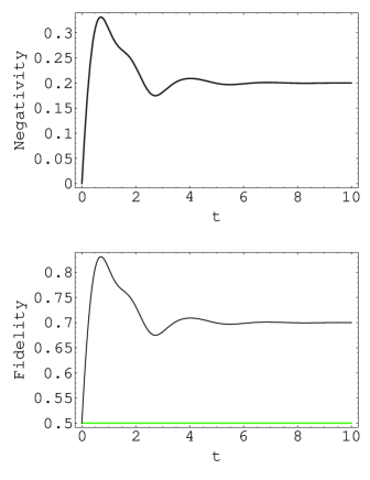
Figure 1: Negativity ${\mathcal{N}}(\rho_{1}(t))$ (upper panel) and the fidelity $F_{\Psi^{[2]}}(\rho_{1}(t))$ (lower panel) are plotted as a function of $t$ with $g=1$, $\gamma=0.3$, $\Delta=1$. The horizontal line in the lower figure shows the minimum fidelity that above it the state is detected to be entangled.

4-2 Case 2

Since, in practice, it is difficult to realize an atom in a pure state, therefore we now suppose that the atom is prepared, initially, in a general mixed state with the diagonal representation

$$\rho^{A}(0)=\lambda|g\rangle\langle g|+(1-\lambda)|e\rangle\langle e|,\qquad\lambda\in[0,1],$$ (28)

but, however, the field is in a pure number state

$$\rho^{F}(0)=|n\rangle\langle n|.$$ (29)

However, we ignore the effect of decoherence and assume that the evolution of the system is unitary. Accordingly, the final state of the system can be obtained as [22, 23]

$$\rho_{n}(t) = \lambda\left(|A_{n}|^{2}|e\rangle\langle e|\otimes|n-1\rangle\langle n-1|+A_{n}B^{\ast}_{n}|e\rangle\langle g|\otimes|n-1\rangle\langle n|\right.$$ (30)

$$+ \left.A^{\ast}_{n}B_{n}|g\rangle\langle e|\otimes|n\rangle\langle n-1|+|B_{n}|^{2}|g\rangle\langle g|\otimes|n\rangle\langle n|\right)$$

$$+ (1-\lambda)\left(|C_{n}|^{2}|e\rangle\langle e|\otimes|n\rangle\langle n|+C_{n}D^{\ast}_{n}|e\rangle\langle g|\otimes|n\rangle\langle n+1|\right.$$

$$+ \left.C^{\ast}_{n}D_{n}|g\rangle\langle e|\otimes|n+1\rangle\langle n|+|D_{n}|^{2}|g\rangle\langle g|\otimes|n+1\rangle\langle n+1|\right),$$

where we have defined

$$A_{n} = -i{\rm e}^{-i\omega_{F}(n-1/2)t}\frac{g\sqrt{n}}{\Omega_{n-1}}\sin{\Omega_{n-1}t},$$

$$B_{n} = {\rm e}^{-i\omega_{F}(n-1/2)t}\left(\cos{\Omega_{n-1}t}+i\frac{\Delta}{2\Omega_{n-1}}\sin{\Omega_{n-1}t}\right),$$

$$C_{n} = {\rm e}^{-i\omega_{F}(n+1/2)t}\left(\cos{\Omega_{n}t}-i\frac{\Delta}{2\Omega_{n}}\sin{\Omega_{n}t}\right),$$

$$D_{n} = -i{\rm e}^{-i\omega_{F}(n+1/2)t}\frac{g\sqrt{n+1}}{\Omega_{n}}\sin{\Omega_{n}t},$$ (31)

where the Rabi frequency $\Omega_{n}$, and the detuning parameter $\Delta$ are the same as before. For the above state the negativity can be expressed as

$${\mathcal{N}}(\rho_{n}(t)) = \frac{1}{2}\left(\sqrt{\lambda^{2}|B_{n}|^{4}+4(1-\lambda)^{2}|C_{n}|^{2}|D_{n}|^{2}}-\lambda|B_{n}|^{2}\right)$$ (32)

$$+ \frac{1}{2}\left(\sqrt{(1-\lambda)^{2}|C_{n}|^{4}+4\lambda^{2}|A_{n}|^{2}|B_{n}|^{2}}-(1-\lambda)|C_{n}|^{2}\right).$$

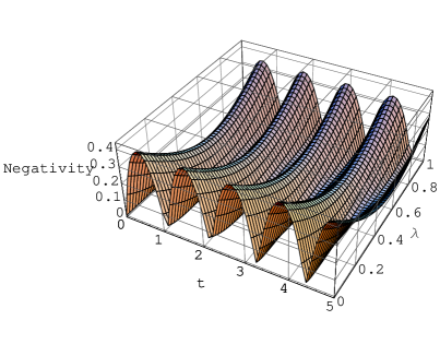
Figure 2: Negativity ${\mathcal{N}}(\rho_{1}(t))$ is plotted as a function of $t$ with $g=1$, $\Delta=1$. .

In order to show the effect of mixing parameter $\lambda$ on the negativity of the system, we plot the negativity ${\mathcal{N}}(\rho_{n}(t))$ as a function of $t$ and $\lambda$ with $g=1$, $\Delta=5$ in figure (2). It is clear from this figure that when purity of this state is decreased, the negativity is also decreased.

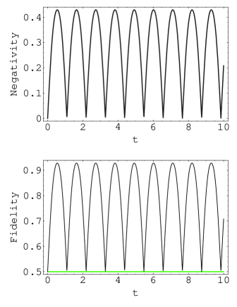
Figure 3: Negativity ${\mathcal{N}}(\rho_{1}(t))$ (upper panel) and the fidelity $F_{\Psi^{[2]}}(\rho_{1}(t))$ (lower panel) are plotted as a function of $t$ with $g=1$, $\Delta=5$ and $\lambda=0$.

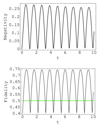
Figure 4: Negativity ${\mathcal{N}}(\rho_{1}(t))$ (upper panel) and the fidelity $F_{\Psi^{[2]}}(\rho_{1}(t))$ (lower panel) are plotted as a function of $t$ with $g=1$, $\Delta=5$ and $\lambda=0.2$.

Now in order to characterize entanglement of this state by using the notion of entanglement witness, we define $|\Psi^{[2]}\rangle$ as equation (26), but here $\{|\Phi^{(0)}\rangle,\;|\Phi^{(1)}\rangle\}$ are two orthonormal vectors in the field space spanned by $\{|n-1\rangle,\;|n\rangle,\;|n+1\rangle\}$ and $\{|{\Phi^{\prime}}^{(0)}\rangle,\;|{\Phi^{\prime}}^{(1)}\rangle\}$ are two orthonormal vectors in the atomic space spanned by $\{|e\rangle,\;|g\rangle\}$. The parametrization of these two sets of vectors are given by equations (2) and (2), respectively. We obtain for the fidelity the following relation

$$F_{\Psi^{[2]}}(\rho_{n}(t)) = \lambda\left(\frac{1}{2}\left(|X_{1}|^{2}|A_{n}|^{2}+|X_{2}|^{2}|B_{n}|^{2}\right)+{\rm Re}{\left(X_{1}^{\ast}X_{2}{\rm e}^{i(\phi_{1}-\phi_{0}+\phi_{1}^{\prime}-\phi_{0}^{\prime})}A_{n}B^{\ast}_{n}\right)}\right)$$

$$+ (1-\lambda)\left(\frac{1}{2}\left(|X_{3}|^{2}|C_{n}|^{2}+|X_{4}|^{2}|D_{n}|^{2}\right)+{\rm Re}{\left(X_{3}^{\ast}X_{4}{\rm e}^{i(\phi_{2}-\phi_{1}+\phi_{1}^{\prime}-\phi_{0}^{\prime})}C_{n}D^{\ast}_{n}\right)}\right),$$

where

$$X_{1} = \cos{\theta_{1}}\cos{\theta_{1}^{\prime}}+\cos{\eta}\sin{\theta_{1}}\sin{\theta_{1}^{\prime}}{\rm e}^{i(\xi_{0}+\xi_{0}^{\prime})},$$

$$X_{2} = \sin{\theta_{1}}\cos{\theta_{2}}\sin{\theta_{1}^{\prime}}+\left(\cos{\eta}\cos{\theta_{1}}\cos{\theta_{2}}{\rm e}^{i\xi_{0}}-\sin{\eta}\sin{\theta_{2}}{\rm e}^{i\xi_{1}}\right)\cos{\theta_{1}^{\prime}}{\rm e}^{i\xi_{0}^{\prime}},$$

$$X_{3} = \sin{\theta_{1}}\cos{\theta_{2}}\cos{\theta_{1}^{\prime}}-\left(\cos{\eta}\cos{\theta_{1}}\cos{\theta_{2}}{\rm e}^{i\xi_{0}}-\sin{\eta}\sin{\theta_{2}}{\rm e}^{i\xi_{1}}\right)\sin{\theta_{1}^{\prime}}{\rm e}^{i\xi_{0}^{\prime}},$$

$$X_{4} = \sin{\theta_{1}}\sin{\theta_{2}}\sin{\theta_{1}^{\prime}}+\left(\cos{\eta}\cos{\theta_{1}}\sin{\theta_{2}}{\rm e}^{i\xi_{0}}+\sin{\eta}\cos{\theta_{2}}{\rm e}^{i\xi_{1}}\right)\cos{\theta_{1}^{\prime}}{\rm e}^{i\xi_{0}^{\prime}}.$$ (34)

Again, by using the MATHEMATICA, we can maximize $F_{\Psi^{[2]}}(\rho_{n}(t))$ with respect to all parameters of the state $|\Psi^{[2]}\rangle$. In figure (3) we have plotted the negativity ${\mathcal{N}}(\rho_{1}(t))$ (upper panel) and the fidelity $F_{\Psi^{[2]}}(\rho_{1}(t))$ (lower panel) as a function of $t$ with $g=1$, $\Delta=5$ and $\lambda=0$. In this case the state of the system is pure and it is clear from the figure that $W_{\Psi^{[2]}}$ enable to detect the entanglement of the system. On the other hand by increasing $\lambda$ from $0$ to $1/2$, the purity of the state is decreased, and the ability of $W_{\Psi^{[2]}}$ to detect entanglement is decreased. For instance, we plot in figure (4) the negativity and the fidelity as a function of $t$ for parameters the same as figure (3) but $\lambda=0.2$. We see that in this case there exist some entangled states that can not be detected by $W_{\Psi^{[2]}}$.

5 Conclusion

We have presented a general parametrization for orthonormal basis of ${\mathbb{C}}^{n}$. This parametrization can be used to construct projector-based witness operators for entanglement detection in the vicinity of pure multipartite states. As an example we have used the method for detecting entanglement between an atom and the single mode of quantized field, described by the Jaynes-Cummings model. We have also compared the detection of witnesses with the negativity of the state, and have shown that in the vicinity of pure stats such constructed witnesses able to detect entanglement of the state.

References

• [1] C. H. Bennett, and S. J. Wiesner, Phys. Rev. Lett. 69, 2881 (1992).
• [2] C. H. Bennett, G. Brassard, C. Crépeau, R. jozsa, A Peres and W. K. Wootters, Phys. Rev. Lett. 70, 1895 (1993).
• [3] C. H. Bennett, D. P. DiVincenzo, J. A. Smolin and W.K. Wootters, Phys. Rev. A 54, 3824 (1996).
• [4] R. F. Werner, Phys. Rev. A 40 4277 (1989).
• [5] A. Peres, Phys. Rev. Lett. 77 1413 (1996).
• [6] M. Horodecki, P. Horodecki and R. Horodecki, Phys. Lett. A 223 1 (1996).
• [7] K. Zyczkowski, P. Horodecki, A. Sanpera and M. Lewenstein, Phys. Rev. A 58 883 (1998).
• [8] K. Zyczkowski, Phys. Rev. A 60 3496 (1999).
• [9] G. Vidal and R. F. Werner, Phys. Rev. A 65 032314 (2002).
• [10] B. M. Terhal, Phys. Lett. A 271 319 (2000).
• [11] B. M. Terhal, Lin. Algebr. Appl. 323 61 (2001).
• [12] B. M. Terhal, Theor. Comput. Sci. 287 313 (2002).
• [13] M. Lewenstein, B. Kraus, J. I. Cirac and P. Horodecki, Phys. Rev. A, 62 052310 (2000).
• [14] P. Diţǎ, J. Phys. A: Math. Gen. 38, 2657 (2005).
• [15] D. M. Greenberger, M. Horne, A. Shimony and A. Zeilinger, Am. J. Phys. 58, 1131 (1990).
• [16] E. T. Jaynes and F. W. Cummings, Proc. IEEE 51 89 (1963).
• [17] W. K. Wootters, Phys. Rev. Lett. 80 2245 (1998).
• [18] M. Bourennane, et al, Phys. Rev. Lett. 92, 087902 (2004).
• [19] E. Schmidt, Math. Annalen. 63, 433 (1906).
• [20] C. W. Gardiner, Quantum Noise, Springer-Verlag, Berlin, (1991).
• [21] Shang-Bin Li and Jing-Bo Xu, Phys. Lett. A 313 175 (2003).
• [22] S. J. Akhtarshenas and M. Farsi, Phys. Scr., 75 608 (2007).
• [23] S. Furuichi and S. Nakamura, J. Phys. A: Math. Gen. 35 5445 (2002).