The inverse problem for the Gross–Pitaevskii equation

Abstract

Two different methods are proposed for the generation of wide classes of exact solutions to the stationary Gross–Pitaevskii equation (GPE). The first method, suggested by the work by Kondrat’ev and Miller (1966), applies to one-dimensional (1D) GPE. It is based on the similarity between the GPE and the integrable Gardner equation, all solutions of the latter equation (both stationary and nonstationary ones) generating exact solutions to the GPE, with the potential function proportional to the corresponding solutions. The second method is based on the “inverse problem” for the GPE, i.e. construction of a potential function which provides a desirable solution to the equation. Systematic results are presented for 1D and 2D cases. Both methods are illustrated by a variety of localized solutions, including solitary vortices, for both attractive and repulsive nonlinearity in the GPE. The stability of the 1D solutions is tested by direct simulations of the time-dependent GPE.

1 Introduction

The Gross–Pitaevskii equation (GPE) provides for an exceptionally accurate description of the dynamics of Bose–Einstein condensate (BEC) [1]. In the general case, the GPE is far from integrability, which was an incentive for the development of various methods for simulations of this equation, including finite-difference [2], split-step [3], and Crank–Nicolson [4] algorithms. An efficient technique for finding stationary solutions to the GPE is based on simulations of the evolution in the imaginary time [5]. A review of numerical methods for the GPE can be found in Ref. [6].

Aside from the numerical solutions, the understanding of results produced by the GPE requires the knowledge of its solutions in an analytical form – approximate or, if possible, exact. A powerful analytical method is provided by the variational approximation [7]. Another approach which simplifies the consideration reduces the three-dimensional (3D) GPE to an effective 1D or 2D form, if the condensate is loaded, respectively, into a cigar-shaped or pancake-shaped trapping potential [8]. If the condensate is trapped in a deep optical-lattice (OL) potential, the continual GPE may be further reduced to its discrete version [9]. In the case of the repulsive nonlinearity, the Thomas–Fermi approximation is known to be very useful [1, 10]. The coupled-mode approximation is adequate for the description of settings based on double- and multi-well potentials [11]. In the case when the GPE contains a rapidly oscillating time dependence, one may apply the averaging approximation [12]. If terms which make the 1D GPE different from the exactly integrable nonlinear Schrödinger equation (NLSE) are small, one may resort to perturbation theory based on the inverse-scattering transform [13, 14]. A number of other approximations have been developed in the context of the GPE, as reviewed in Ref. [15].

Although exact solutions of the GPE are rare, they are useful in those cases when they are available (see. e.g., Ref. [16]). An example is a family of exact stationary periodic solutions to the 1D GPE with a specially devised periodic potential, written in terms of elliptic functions. This analysis was performed for both cases of the repulsive [17] and attractive [18] nonlinearity in the GPE, see also Ref. [19]. Exact solutions were also found for dark-soliton trains representing the supersonic flow of the condensate [20]. Exact localized solutions are known in the case when the nonlinearity coefficient is represented by a delta-function of the spatial coordinate [21] and by a symmetric pair of delta-functions [22]. In fact, the latter configuration provides for an exact solution to the spontaneous-symmetry-breaking problem. Upon a proper change of the notation, the GPE may be interpreted as the NLSE for spatial optical beams in nonlinear waveguides [23]. Accordingly, the exact solutions found in terms of the GPE may also find applications to nonlinear optics.

The purpose of this work is to propose two methods for generating exact solutions to the GPE, together with potentials which support them. The first method is based on the idea proposed by Kondrat’ev and Miller [30] more than 40 years ago, namely, using known solutions of nonlinear equations as potentials for other equations (a somewhat similar method was later proposed for the analysis of self-trapped states in nonlinear optics [31]). We apply it by noting that the 1D time-independent GPE with the potential term is equivalent to a stationary Gardner equation (GE), alias an extended Korteweg–de Vries (KdV) equation, containing both quadratic and cubic nonlinearities, if the solution is proportional to the potential. Thus, one can obtain a solution to the GPE, along with the necessary potential, from any solution of the GE.

The second method is based on the consideration of an inverse problem, aiming to construct an appropriate potential for a given wave-function ansatz representing an appropriate solution. The inverse problem is relevant because it may be relatively easy to engineer the needed trapping potential, using external magnetic and optical fields [24]. Recent experiments have demonstrated that, using a rapidly moving laser beam focused on the condensate, one can “paint” practically any desired time-average potential profile in 1D and 2D settings [25]. A similar approach was developed in a different physical setting, with the objective to find models of nonlinear dynamical chains admitting exact solutions for traveling discrete pulses in an analytical form [26]. By means of this approach, we produce a number of novel 1D and 2D stationary solutions. The stability of the 1D solutions obtained by both above-mentioned methods is tested in direct simulations.

The paper is organized as follows. In Section 2, we elaborate the Kondrat’ev–Miller method in the 1D case and perform the stability test of the localized modes. We show that stationary solutions of the GPE may be constructed using not only stationary, but also nonstationary solutions of the GE. In the latter case, the use of the formal temporal variable in the GE makes it possible to obtain a wide family of stationary solutions and supporting potentials which depend on a continuous parameter, the relation between them being different from the proportionality. In the same section, we present the inverse method in the 1D case. The stability of these solutions is tested via direct simulations of the time-dependent GPE. In Section 3, we construct exact solutions to the GPE in the 2D case (the test of their stability will be reported elsewhere). In particular, we construct anisotropic solutions, using the so-called lump solitons of the Kadomtsev–Petviashvili equation (KP1) as the respective ansatz, axisymmetric states with the Gaussian radial profile, and vortices with topological charges $1$ and $2$. The paper is concluded by Section 4.

2 Exact solutions of the one-dimensional Gross–Pitaevskii equation

The scaled form of the 1D GPE for complex wave function $\varphi(\xi,t)$ is well known [1]:

$$i\varphi_{t}+\mu\varphi=-\varphi_{\xi\xi}+u(\xi)\varphi+\sigma|\varphi|^{2}\varphi,$$ (1)

where $u(\xi)$ is the trapping potential, $\sigma=+1$ or $-1$ corresponding to the repulsive and attractive interactions between atoms. The constant $\mu$ in Eq. (1) is the chemical potential, the objective being to find stationary solutions corresponding to a given value of $\mu$. If Eq. (1) is derived from the underlying GPE for the 3D condensate, the temporal variable $t$ and spatial coordinate $\xi$, together with function $\varphi$ and normalized potential $u(\xi)$, are related to their counterparts measured in physical units, $T,X$ and $\Psi$, as follows: $t\equiv T\left(\pi^{2}\hslash/md^{2}\right)$, $\xi\equiv\pi X/d$, and

$$\Psi(X,R,T)=\sqrt{\frac{\pi}{2\left|a_{s}\right|d^{2}}}\,\varphi(\xi,t)\exp{\left(-i\omega_{\perp}T-\frac{\omega_{\perp}m}{2\hbar}R^{2}\right)},$$ (2)

$$U(X)=\frac{1}{m}\left(\frac{\pi\hbar}{d}\right)^{2}u(\xi),$$ (3)

where $m$ is the atomic mass, $d$ is a longitudinal scale determined by the axial potential, $a_{s}$ is the $s$-wave scattering length, while $\omega_{\perp}$ and $R$ are the transverse trapping frequency and radial coordinate. If $m$ is taken for ⁸⁷Rb, and $d=1.5$ $\mathrm{\mu}$m, then $t=1$ and $\xi=1$ correspond, in physical units, to $T\approx 0.3\$ms and $X\approx 0.5$ $\mathrm{\mu}$m, respectively. Finally, the number of atoms in the condensate is

$$N\equiv 2\pi\int\limits_{0}^{\infty}R\,dR\int\limits_{-\infty}^{+\infty}\left|\Psi(X,R,T)\right|^{2}dX\equiv\frac{\pi a_{\perp}^{2}}{2\left|a_{s}\right|d}\int\limits_{-\infty}^{+\infty}|\varphi(\xi)|^{2}d\xi,$$ (4)

where the transverse-trapping size is $a_{\perp}=\sqrt{\hbar/m\omega_{\perp}}$.

2.1 Construction of stationary solutions by the Kondrat’iev–Miller method

Looking for real stationary solutions to Eq. (1), we arrive at equation

$$\varphi^{\prime\prime}+\mu\varphi=u(\xi)\varphi+\sigma\varphi\,^{3},$$ (5)

with the prime standing for $d/d\xi$. Particular exact solutions to Eq. (5) can be obtained by way of the approach developed in Ref. [30]. To this end, parallel to Eq. (5), one should consider the stationary GE (see [28, 33] and references therein):

$$\phi^{\prime\prime}-V\phi=-\alpha\phi\,^{2}+\sigma\phi\,^{3},$$ (6)

where $V$ and $\alpha$ are constants. It is well known that exact solutions to Eq. (6) can be found in terms of the Jacobi’s elliptic functions. We chose one of such solutions and denote it $\Phi(\xi)$. Then, the quadratic term in Eq. (6) is formally factorized, and the first multiplier is replaced by $\Phi(\xi)$, i.e. $\phi^{2}\equiv\phi\cdot\phi\rightarrow\Phi(\xi)\phi$. By substituting this into Eq. (6), one obtains:

$$\phi^{\prime\prime}-V\phi=-\alpha\Phi(\xi)\phi+\sigma\phi\,^{3}.$$ (7)

Obviously, this equation is immediately satisfied with $\phi=\Phi(\xi)$. From here it follows that there is the one-to-one correspondence between Eqs. (5) and (7):

$$\varphi\longleftrightarrow\phi,\quad\mu\longleftrightarrow-V,\quad u(\xi)\longleftrightarrow-\alpha\Phi(\xi).$$ (8)

Thus, Eq. (5) gives rise to the exact solution, $\varphi(\xi)=\Phi(\xi)$, with chemical potential $-V$, for the external potential

$$u(\xi)=-\alpha\Phi(\xi).$$ (9)

2.2 Stationary solutions in the case of the repulsive nonlinearity

An illustrative example – the “fat soliton” of the Gardner equation. In the case of the repulsive atomic interactions, which corresponds to $\sigma=+1$ in Eq. (1), the approach outlined above may be illustrated using a particular solution to Eq. (6) in the form of so-called “fat soliton” [33]):

$$\Phi(\xi)=\frac{\alpha\nu}{3}\left[\tanh{\left(\xi/\Delta+\theta\right)}-\tanh{\left(\xi/\Delta-\theta\right)}\right],$$ (10)

$$\theta=(1/4)\ln\left[(1+\nu)/(1-\nu)\right],~{}\Delta=3\sqrt{2}/(\alpha\nu),~{}V=(2/9)(\alpha\nu)^{2},$$ (11)

with free parameters $\alpha$ and $\nu$, the latter one taking values $0<\nu<1$. The front and rear slope of the fat soliton, $\Delta$, depends monotonously on $\nu$, decreasing from infinity to $\Delta_{\min}=3\sqrt{2}/\alpha$ when $\nu$ varies from $0$ to 1. The width of the soliton, $L$, i.e. the distance between its front and rear segments at the half-minimum level, $\Phi(\xi)=\Phi_{\max}/2$, is

$$L=\frac{3\sqrt{2}}{\alpha\nu}\ln{\left[2+\left(1-\nu^{2}\right)^{-1/2}+\sqrt{\left(2+\left(1-\nu^{2}\right)^{-1/2}\right)^{2}-1}\,\right]}.$$ (12)

At $\nu\rightarrow 0$, the fat soliton reduces to the bell-shaped KdV soliton, whose width is given by $L_{\mathrm{KdV}}=3\sqrt{2}\ln{\left(3+\sqrt{8}\right)}/(\alpha\nu)$. In the other limit, $\nu\rightarrow 1$, it reduces to the “table-top soliton” (a $\Pi$-shaped mode) with $L\approx 2\Delta\theta\approx-3\sqrt{2}\ln{\left[{(1-\nu)/\nu}\right]}/(2\alpha\nu)$. The minimum width, $L_{\min}\approx 10.1/\alpha$, is attained at $\nu\approx 0.892$. The local density corresponding to normalized solution (10), $|\Phi/\alpha|^{2}$, along with the corresponding normalized potential, $u/\alpha^{2}$, in the stationary GPE for which one has $\Phi(\xi)$ as the exact solution, are shown in Fig. 1 for several values of free parameter $\nu$.

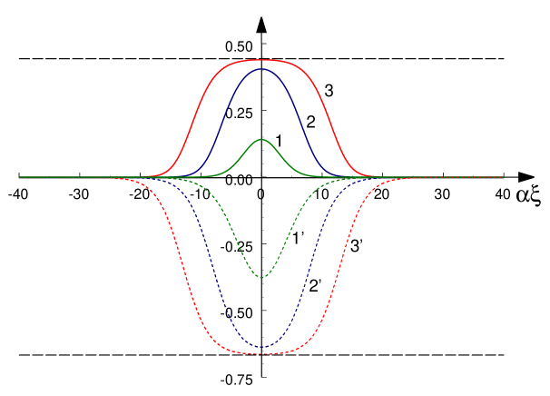
Figure 1: Normalized density $|\Phi(\xi)/\alpha|^{2}$ corresponding to solution (10) (solid lines), and the corresponding normalized potential $u(\xi)/\alpha^{2}$ (broken lines), as functions of $\alpha\xi$. Lines $1$ and $1^{\prime}$ pertain to $\nu=0.9$; lines $2$ and $2^{\prime}$ – to $\nu=0.999$; lines $3$ and $3^{\prime}$ – to $\nu=0.99999$. The horizonal dashed lines show limit values of the solution and potential function for the “table-top soliton”.

The dimensionless norm of exact solution (10), which is proportional to the number of particles in the underlying BEC, according to Eq. (4), is

$$N_{\mathrm{1D}}=\int\limits_{-\infty}^{+\infty}|\varphi(\xi)|^{2}\,d\xi=4\sqrt{2}\alpha\nu\left[\frac{1}{2\nu}\ln{\left(\frac{1+\nu}{1-\nu}\right)}-1\right].$$

As follows from here, $N_{\mathrm{1D}}$ is proportional to $\alpha$, while $\nu$ may be treated as a free parameter which determines the shape of the potential and the corresponding solution. The chemical potential of the solution, $\mu=-V$, is also determined by constants $\alpha$ and $\nu$, see Eq. (11).

Because wave function (10) has no zeros, it may represent the ground state in the corresponding potential, with chemical potential $\mu=-\left(2/9\right)\left(\alpha\nu\right)^{2}\$[see Eq. (11)]; whether there exist higher-order bound states with larger discrete eigenvalues of $\mu$ within this nonlinear problem, remains an open question. Although it is plausible that this solution is stable, it is relevant to test its dynamics, under the action of perturbations, in direct simulations of the time-dependent equation (1). This was done by means of the Yunakovsky’s method [29] in a sufficiently large domain with periodic boundary conditions (description of the method is presented in the Appendix). Examples are shown in Fig. 2 for cases when the amplitude was initially reduced or increased by $10\%$ against the stationary value.

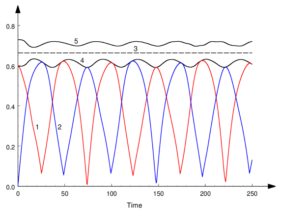
Figure 2: The time dependence of perturbed solution (10) in the model with the repulsive nonlinearity, when the initial amplitude is $10\%$ smaller than needed for the stationary solution. Line 1 – max${}_{\xi}|\mathrm{Re}\left\{\varphi(\xi,t)\right\}|$, line 2 – max${}_{\xi}|\mathrm{Im}\left\{\varphi(\xi,t)\right\}|$. Horizontal line 3 designates the constant amplitude of stationary soliton (10) with $\nu=0.99999$. Lines 4 and 5 show the time dependence of max${}_{\xi}|\varphi(\xi,t)|$ in the cases when the soliton’s amplitude was initially reduced (line 4) or increased (line 5) by $10\%$ against the stationary value.

As seen from the figure, the amplitude of the so perturbed solution varied in time within the same $10\%$, while its spatial shape was preserved. It is also seen that the perturbation induced oscillations between the real and imaginary parts of the solution, i.e. shifted its chemical potential. In the course of the simulations, the norm of the solution was preserved with relative accuracy $\sim 10^{-7}$. The latter fact attests to the robustness of the ground state: under the action of this sufficiently strong perturbation, it features no loss through emission of radiation.

Using the above physical estimates for BEC, it is easy to estimate physical parameters of BEC states corresponding to the fat-soliton solutions. For instance, the outermost configuration in Fig. 1 represents to the potential well of the depth $\simeq 1$ recoil energy corresponding to $d=1.5$ $\mathrm{\mu}$m, and width $L\simeq 30$, which is $\simeq 15$ $\mathrm{\mu}$m in physical units (see above). These values are quite realistic for the experiment [1, 24, 25]. Further, taking an experimentally relevant values of $a_{s}=5$ nm and $a_{\perp}=3$ $\mathrm{\mu}$m, Eq. (4) yields the largest number of ⁸⁷Rb atoms which may form the fat soliton, $N\simeq 30,000$. This estimate shows that the constructed soliton solution is quite relevant to the experiment. Finally, the period of large-amplitude oscillations of the perturbed stable state, shown in Fig. 2, is $\sim 100$ ms.

Other stationary solutions related to the Gardner equation. To consider various exact solutions to Eq. (6), one may write the equation in the “energy conservation” form, $(X^{\prime})^{2}/2+P(X)=E$, where $X\equiv\phi/\alpha$, $E$ is a constant of integration, and $P(X)$ is the effective potential,

$$P_{+}(X)=-\left(\sigma/4\right)\alpha^{2}X^{2}\left[\left(X-2\sigma/3\right)^{2}+2\sigma W-4/9\right],$$ (13)

with $W\equiv V/\alpha^{2}$. It is shown in Fig. 3 for $\sigma=1$.

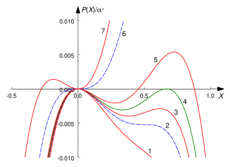
Figure 3: Normalized polynomial $P(X)/\alpha^{2}$ defined in Eq. (13) with $\sigma=1$ at different values of $W$: line $1$ – for $W=9/32$, line $2$ – for $W=1/4$, line $3$ – for $W=17/72$, line $4$ – for $W=2/9$, line $5$ – for $W=1/5$, line $6$ – for $W=0$, and line $7$ – for $W=-2/9$.

For $W>1/4$, the polynomial has a single real maximum at $X=0$, hence neither periodic nor solitary solutions are possible. At $W<1/4$, it has three real extrema, at points $X=0,~{}(1/2)(1-\sqrt{1-4W}),~{}(1/2)(1+\sqrt{1-4W})$. In that case, first appears a depression-type solitary solution, in the form of a “bubble” against the constant background value of the field, $\phi_{0}=(\alpha/2)\left(1+\sqrt{1-4V/\alpha^{2}}\right)$. The typical potential profile corresponding to the “bubble” is depicted by the line 3 in Fig. 3.

At $W=2/9$, the potential becomes symmetric, as shown in Fig. 3 by line 4. Solution (10) with $\nu=1$ corresponds exactly to this case. For smaller values of $W$, when it varies from $2/9$ to $0$, the right maximum of the potential function becomes taller then the left one, making it possible to have bright solitons with the zero background. They correspond to solution (10) with $\nu<1$. The solution vanishes at $W\rightarrow+0$, i.e. $\nu\rightarrow+0$. For $W<0$, the left maximum of the potential shifts from the origin to the left, see Fig. 3). In this case, solitons exist against the negative background, with $\phi_{0}=(\alpha/2)\left(1-\sqrt{1-4V/\alpha^{2}}\right)$.

Periodic solutions of Eq. (6) can be analyzed similarly. The corresponding stationary solutions of the GPE can be readily obtained by means of the method described above, in terms of elliptic functions, similar to the periodic solutions reported in Ref. [19].

2.3 Stationary solutions in the case of the attractive nonlinearity

In the case of the attractive nonlinearity, i.e. $\sigma=-1$ in Eq. (5), the potential function is different from that shown in Fig. 3. It is shown in Fig. 4 in two different scales, as it is impossible to display all details using a single scale. For $W\geq-1/4$, three possible real extrema of this polynomial are located at points

$$X=0,\quad-\frac{1}{2}\left(1-\sqrt{1+4W}\right),\quad-\frac{1}{2}\left(1+\sqrt{1+4W}\right),$$

otherwise the polynomial has a single real minimum at $X=0$, hence solitary solutions do not exist for $W<-1/4$.

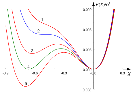
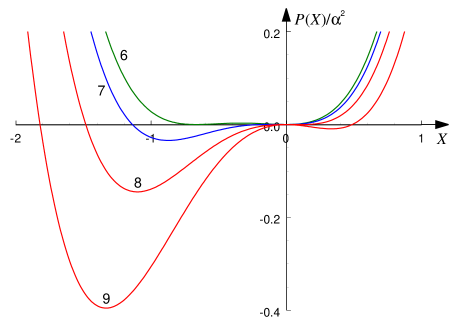
a)	b)

Figure 4: Normalized polynomial $P_{-}(X)/\alpha^{2}$ defined by Eq. (13) with $\sigma=-1$ for different values of $W$. Frame (a): line $1$ – for $W=-0.26$, line $2$ – for $W=-0.25$, line $3$ – for $W=-0.23$, line $4$ – for $W=-0.22$, and line $5$ – for $W=-0.21$. Frame (b) uses a different scale: line $6$ – for $W=-0.22$ [the same as line 4 in (a)], line $7$ – for $W=-0.11$, line $8$ – for $W=0.11$, and line $9$ – for $W=0.44$.

The first solitary-type solution emerges at $W=-1/4$. In this case, the potential still has only one minimum at $X=0$, but the inflexion point appears at $X=-1/2$ (the corresponding potential function is shown in Fig. 4 by line 2). A particular solution corresponding to $W=-1/4$ represents the algebraic soliton sitting on top of a pedestal (constant-value background), as a solution to Eq. (5) with free parameter $\alpha$ and $V=-\mu=-\alpha^{2}/4$:

$$\Phi(\xi)=\frac{\alpha}{2}\left(\frac{4}{3}\frac{1}{1+\alpha^{2}\xi^{2}/18}-1\right).$$ (14)

At $W>-1/4$, one more minimum appears in the potential profile (see, e.g., line 3 in Fig. 4). In this case, two families of solitons on a pedestal are generated by Eq. (6):

$$\Phi_{\pm}(\xi)=\alpha\nu\left\{1-\frac{3(1+2\nu)}{1+3\nu\pm\sqrt{1+3\nu/2}\cosh{\left[\alpha\xi\sqrt{-\nu(1+2\nu)}\,\right]}}\right\},$$ (15)

where $\nu$ is a free parameter ranging between $-1/2$ and $0$, and $V=-\mu=\alpha^{2}\nu(1+\nu)$. The local densities corresponding to solution $\Phi_{+}(\xi)$ has the form of a double dark soliton (with two zeros), whereas solution $\Phi_{-}(\xi)$ is shaped as a bump on top of the pedestal. The local densities corresponding to solutions (15), along with the respective potentials, for which these are exact solutions to the GPE, are shown in Fig. 5 for $\nu=-5/12$.

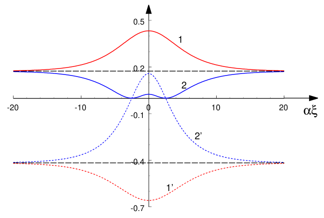
Figure 5: Solutions (15) in terms of $(\Phi_{\pm}/\alpha)^{2}$ (solid lines), and respective normalized potentials $u/\alpha^{2}$ (broken lines) are shown as functions of normalized coordinate $\alpha\xi$. Lines $1$, $1^{\prime}$ and $2$, $2^{\prime}$ pertain, respectively, to signs plus and minus in Eq. (15). In both cases, $\nu=-5/12$.

When $W$ increases further and becomes equal to $-2/9$, potential function (13) becomes symmetric with respect to the vertical line $X=-1/3$ (see line 4 in Fig. 4), getting then asymmetric, with the left minimum falling deeper than the right one when $W$ increases further (see, e.g., line 5 in Fig. 4). For the particular case of $W=-2/9$, solutions (15) reduce to

$$\Phi(\xi)=-\frac{\alpha}{3}\left[1\pm\sqrt{2}\mathrm{sech}{\left(\frac{\alpha\xi}{\sqrt{3}}\right)}\right].$$

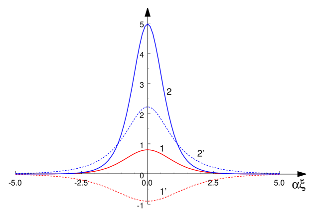
Figure 6: $(\Phi_{\pm}/\alpha)^{2}$ for solutions (16) with $\nu=1$ (solid lines), and the corresponding normalized potentials, $u/\alpha^{2}$ (broken lines), as functions of $\alpha\xi$. Lines $1$, $1^{\prime}$ and $2,$ $2^{\prime}$ pertain, respectively, to signs $+$ and $-$ in Eq. (16).

For $W$ ranging between $-2/9$ and $-1/9$, the potential function (13) becomes again asymmetric, as mentioned above, while the corresponding solutions are still given by Eq. (15) with $-1/3\leq\nu\leq 0$. They remain unstable, because of the nonzero background.

At $W=-1/9$, the maximum and minimum of the potential merge at $X=0$. Another inflexion point emerges in the potential profile in this case [see line 7 in Fig. 4(b)]. The corresponding solution to Eq. (6) is an algebraic soliton with $V=-\mu=0$ and zero background,

$$\Phi(\xi)=-\frac{4\alpha}{3}\frac{1}{1+2\alpha^{2}\xi^{2}/9}.$$

However, as follows from Eq. (9), this solution corresponds to the maximum of the physical potential, hence its is unstable (which was confirmed by direct simulations).

For $W>-1/9$, two families of exponentially localized solitons are generated by Eq. (6):

$$\Phi_{\pm}(\xi)=\frac{3\alpha\nu^{2}}{1\pm\sqrt{1+9\nu^{2}/2}\cosh{(\nu\alpha\xi)}},$$ (16)

where free parameter $\nu\geq 0$ determines the inverse width of the soliton, and $V=-\mu=(\alpha\nu)^{2}$. These solutions and corresponding potentials are shown in Fig. 6 for $\nu=1$. As follows from Eq. (9), solution $\Phi_{-}(\xi)$ is unstable, as it represents a soliton sitting at the potential maximum. However, solution $\Phi_{+}(\xi)$ is trapped in the minimum of the attractive potential, hence it may be stable. At $\nu\rightarrow 0$, the latter solution smoothly vanishes, whereas the unstable one reduces to the above-mentioned unstable algebraic soliton.

The stability of all the solutions found in the model with the attractive nonlinearity was tested via direct simulations of Eq. (1). First, the expected instability of the solutions on the pedestal and localized modes placed at the maximum of the potential was corroborated. In the former case, the modulational instability of the background leads to the formation of a chaotic “gas” of interacting solitons. An examples of such instability onset is shown in Fig. 7, which shows a spatial distribution of the density, $|\varphi(\xi)|^{2}$, at different moments of time when the spatial period is $L=128$. In the latter case, small random perturbations may either cause the soliton to roll down from the unstable position (see an example in Fig. 8a), or split – symmetrically (see Fig. 8b), or sometimes asymmetrically (see Fig. 8c) – into two solitons moving in opposite directions. In particular, the splitting was, naturally, observed under the action of an initial perturbation which made the amplitude of the unstably pinned soliton smaller, hence making it more similar to a quasi-linear wave packet which is subject to the splitting by the potential barrier. In fact, the strongly asymmetric splitting may be realized as a result of strong emission of radiation from the unstable soliton and self-retrapping of the emitted wave packet into a small-amplitude soliton. Because the simulations were run in the domain with periodic boundary conditions, we also observed that, in the case of the splitting of the unstable soliton into two, like in Figs. 8b and 8c, the secondary solitons survived in the course of numerous head-on collisions in the course of their circular motion. If the instability gave rise to a moving soliton and a radiation wave-train, the secondary interactions between them would not destroy the soliton either.

Also in agreement with the expectation formulated above, the numerical solutions demonstrate the stability of solitons $\Phi_{+}$ gives by Eq. (16). In this case, the amplitude of the perturbed soliton, $\mathrm{\max}_{\xi}|\varphi(\xi)|$, varies in time around some average value, as shown by lines 4 and 5 in Fig. 9, and remains within the same range of the deviation from the

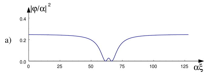
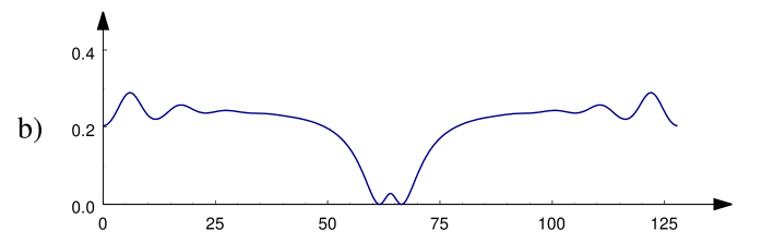
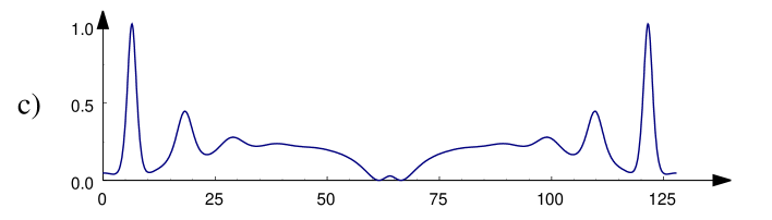
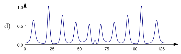
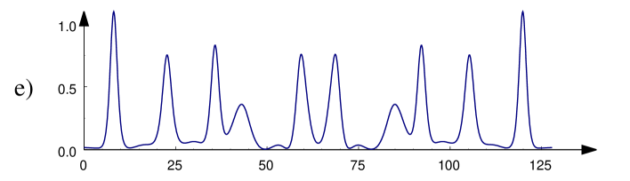
Figure 7: An example of the instability development for the algebraic soliton on a pedestal, given by Eq. (14) in the model with the self-attraction: (a) – $t=0$; (b) – $t=30$; (c) – $t=40$; (d) – $t=80$; (e) – $t=100$ (the vertical scale in the three latter cases is compressed by a factor of $2.5$).

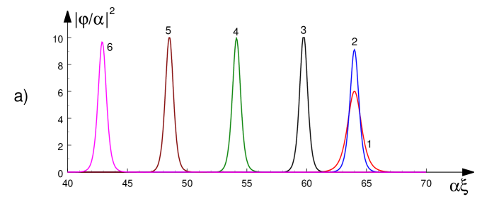
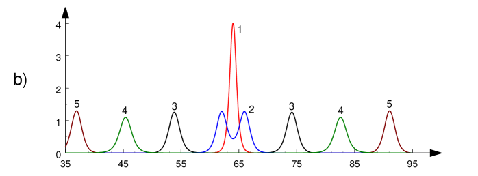
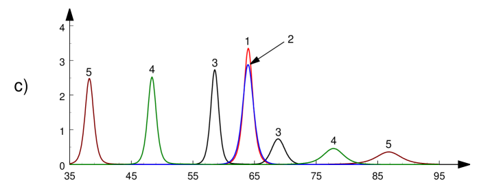
Figure 8: The evolution of a disturbed exponentially localized soliton $\Phi_{-}$ from Eq. (16) (only a part of the total spatial period of $L=128$ is shown). Panel (a) – the initial amplitude is $10\%$ greater than the stationary value corresponding to $\alpha=\nu=1$ (line 1 – $t=0$, line 2 – $t=12$, line 3 – $t=16$, line 4 – $t=18$, line 5 – $t=20$, and line 6 – $t=22$). Panel (b) – initial amplitude is $10\%$ smaller than the stationary value (line 1 – $t=0$, line 2 – $t=2$, line 3 – $t=6$, line 4 – $t=10$, and line 5 – $t=14$). Panel (c) shows the evolution of initially undisturbed soliton (16), with $\alpha=1$ and $\nu=0.675$, under the influence of small errors of the numerical truncation (line 1 – $t=0$, line 2 – $t=8$, line 3 – $t=10$, line 4 – $t=12$, and line 5 – $t=14$).

stationary value as the initial perturbation. The stability of these solitons is similar to that which was demonstrated above for the table-top soliton in Fig. 2 in the model with repulsive nonlinearity.

Figure 9: The evolution of perturbed solution $\Phi_{+}$ from Eq. (16) in the model with the attractive nonlinearity, when the amplitude of the initial perturbation was $10\%$ smaller than needed for the stationary solution. Line 1 – max${}_{\xi}|\mathrm{Re}\left\{\varphi(\xi,t)\right\}|$; line 2 – max${}_{\xi}|\mathrm{Im}\left\{\varphi(\xi,t)\right\}|$. Horizontal line 3 shows the constant amplitude of stationary soliton $\Phi_{+}$ with $\nu=1$; lines 4 and 5 show the time dependence of max${}_{\xi}|\varphi(\xi,t)|$ in cases when the soliton’s amplitude was reduced (line 4) or increased (line 5) by $10\%$ against the stationary value.

2.4 Other stationary solutions obtained from nonstationary solutions of the auxiliary Gardner equation

The nonstationary version of GE (6),

$$\phi_{\tau}+\left(c\phi+\phi_{\xi\xi}-\phi^{2}-\sigma\phi^{3}\right)_{\xi}=0.$$ (17)

can also be used for the purpose of generating stable stationary solutions to the GPE [note that here, in comparison with Eq. (6), we set $\alpha=-1$]. We stress that formal temporal variable $\tau$ in this equation has nothing to do with physical time $t$ in Eq. (1).

Equation (17) is tantamount to the integrable modified KdV equation [28, 32, 35, 34]. It may be formally integrated once in $\xi$ and cast in the following form:

$$c\phi+\frac{\partial^{2}\phi}{\partial\xi^{2}}-\Phi(\xi,\tau)\phi-\sigma\phi^{3}=-\left[\frac{1}{\Phi(\xi,t)}\frac{\partial}{\partial\tau}\int_{0}^{\xi}\Phi(x^{\prime},\tau)\,dx^{\prime}\right]\phi,$$ (18)

where $\Phi(x,\tau)$ is one of the particular nonstationary solutions to Eq. (17). The term on the right-hand side of Eq. (18) can be combined with term $\Phi(\xi,\tau)\phi$ on the left-hand side, to generate the stationary GPE in the form of Eq. (5) with $c=\mu$ and potential $u(\xi,\tau)$ which depends on free parameter $\tau$:

$$u(\xi,\tau)=\Phi(\xi,\tau)-\frac{1}{\Phi(\xi,\tau)}\frac{\partial}{\partial\tau}\int_{0}^{\xi}\Phi(x^{\prime},\tau)\,dx^{\prime},$$ (19)

cf. Eq. (9) for the case when the stationary GE was used. It is worthy to stress that, in the present case, the solution and the potential which support it are no longer proportional to each other.

As an example, we take, following Ref. [35], a solution to nonstationary GE (17) with $\sigma=1$, which describes disintegration of the initial configuration into two fat solitons:

$$\Phi(\xi,\tau)=\frac{\nu_{1}^{2}-\nu_{2}^{2}}{3}\left(\frac{1}{Z_{2+}-Z_{1+}}-\frac{1}{Z_{2-}-Z_{1-}}\right),$$ (20)

where

$$Z_{1\pm}\equiv\nu_{1}\tanh{\left\{\frac{\nu_{1}\sqrt{2}}{6}\left[\xi-\left(-\mu+\frac{2\sqrt{2}}{27}\nu_{1}^{2}\right)\tau\pm\delta_{1}\right]\right\}},$$ (21)

$$Z_{2\pm}\equiv\nu_{2}\coth{\left\{\frac{\nu_{2}\sqrt{2}}{6}\left[\xi-\left(-\mu+\frac{2\sqrt{2}}{27}\nu_{2}^{2}\right)\tau\pm\delta_{2}\right]\right\}},$$ (22)

$$\delta_{1,2}=\left(2\nu_{1,2}\right)^{-1}\ln\left[\left(1+\nu_{1,2}\right)/\left(1-\nu_{1,2}\right)\right].$$ (23)

Two examples of these solutions are shown in Fig. 10 for a fixed value of $\nu_{1}=0.75$ and two different values of the other parameter, $\nu_{2}=0.8$ and $0.999$. The configuration shown in Fig. 10(b) actually represents a pair of table-top Gardner solitons (10) with different parameters. Solution (20)–(23) may be treated as a continuous family (parameterized by $\tau$) of stationary solutions to Eq. (5), with the corresponding potential produced by Eqs. (20)–(23).

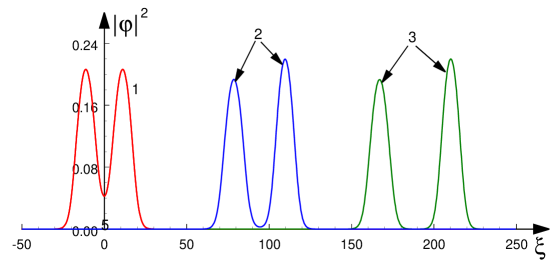
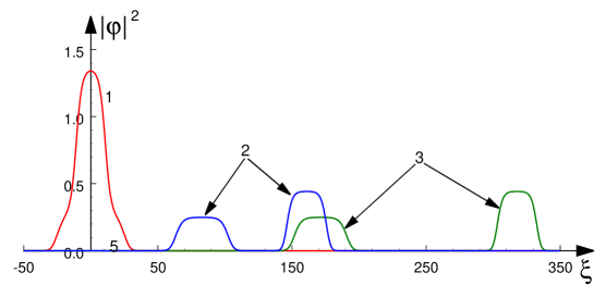
Figure 10: Solutions to the nonstationary Gardner equation (17) with $c=0$ and $\sigma=1$, which describe disintegration of the initial configuration into a pair of “fat solitons”. They emerge with parameters $\nu_{1}=0.75$, $\nu_{2}=0.8$ in (a), and $\nu_{1}=0.75$, $\nu_{2}=0.999$ in (b). Lines 1, 2, and 3 correspond, respectively, to $\tau=0$, $\tau=1500,$ and $\tau=3000$.

To conclude this subsection, it is relevant to mention exact nonstationary solutions in the form of breathers, for Gardner equation (17) corresponding to the GPE with the attractive nonlinearity ($\sigma=-1$) [34]. Such breathers look as two periodically interacting exponentially localized solitons, or as envelope solitons of the NLSE. At any fixed value of $\tau$ in Eq. (17), the breathers generate, as outlined above, exact stationary solutions of the GPE with the corresponding potentials given by Eq. (19).

2.5 Reconstruction of the supporting potential in the GPE for an arbitrary matter-wave distribution

An arbitrary distribution of the stationary matter-wave field, $\varphi(\xi)$, can be made an exact solution to stationary GPE (5), if the potential in the equation is chosen as

$$u(\xi)=\frac{\varphi^{\prime\prime}}{\varphi(\xi)}-\sigma\varphi^{2}(\xi)+\mu.$$ (24)

Below, we demonstrate that this, seemingly “trivial”, approach may also produce essential results.

An example: the Gaussian profile of the matter wave. First, we take a Gaussian matter-wave pulse, which is the case of obvious interest to applications, $\varphi(\xi)=A\exp{[-(\xi/l)^{2}]}$. Substituting this into Eq. (24), one finds:

$$u(\xi)=\frac{2}{l^{2}}\left(2\frac{\xi^{2}}{l^{2}}-1\right)-\sigma A^{2}\exp{[-2(\xi/l)^{2}]}+\mu.$$

The trial solution, $\varphi(\xi)$, and the corresponding potential can be presented in the dimensionless form:

$$F(\zeta)=\exp{(-\zeta^{2})},\quad v_{e}(\zeta)=\frac{2}{S^{2}}\left(2\zeta^{2}-1\right)-\sigma\exp{(-2\zeta^{2})}+M,$$ (25)

where $\zeta=\xi/l$, $F(\zeta)=\varphi(\zeta)/A$, $v_{e}(\zeta)=u(\zeta)/A^{2}$, $S=Al$, $M=\mu/A^{2}$. While $F(\zeta)$ does not contain any parameter, the dimensionless potential depends on two independent constants, $S$ and $M$, for each sign of $\sigma=\pm 1$. Figure 12 shows the squared normalized solution, $F^{2}(\zeta)$, and the corresponding potentials for both signs of $\sigma$, as given by Eq. (25) for several values of $S$ and $M=0$. Note that, in the case displayed in Fig. 12c, the potential corresponding to the GPE with the self-attraction nonlinearity ($\sigma=-1$) features a double-well shape. As follows from Eq. (25), such a shape may occurs only in the case of $\sigma=-1$, provided that $S$ exceeds a threshold value, $S_{\mathrm{thr}}=\sqrt{2}$.

A derivative-Gaussian profile of the matter wave. Trial function $\varphi(\xi)$ used above is an even function of $\xi$ without nodes, which, apparently, represents the ground state for the nonlinear GPE with the given potential. Here we aim to consider another example, when the trial function is chosen as an odd one, with a single node, thus representing the first excited state. To this end, we take $\varphi(\xi)=A\xi\exp\left[{-}\left({\xi/l}\right){{}^{2}}\right]$ and derive the corresponding potential from Eq. (24):

$$u(\xi)=\frac{2}{l^{2}}\left(2\frac{\xi^{2}}{l^{2}}-3\right)-\sigma A^{2}\xi^{2}\exp{[-2(\xi/l)^{2}]}+\mu.$$

It is again convenient to present the trial solution, $\varphi(\xi)$, and the corresponding potential in the dimensionless form:

$$F(\zeta)=-\zeta\exp{(-\zeta^{2})},\quad v_{e}(\zeta)=\frac{2}{S^{2}}\left(2\zeta^{2}-3\right)-\sigma\zeta^{2}\exp{(-2\zeta^{2})}+M,$$ (26)

where, this time, $\zeta=\xi/l$, $F(\zeta)=\varphi(\zeta)/A$, $v_{e}(\zeta)=u(\zeta)/A^{2}l^{4}$, $S=Al^{2}$, and $M=\mu/(Al)^{2}$. Plots corresponding to this trial function and the supporting potentials are displayed in Fig. 12 for $M=0$ and both signs of the parameter $\sigma$. Apparently, function $F(\zeta)$ represents the first excited eigenmode in the corresponding potential well $v_{e}(\zeta)$. Note that, as it follows from Eq. (26), the trapping potential has a single-well structure at $S\leq S_{\mathrm{thr}}^{+}\equiv 2$ for $\sigma=+1$, and at $S\leq S_{\mathrm{thr}}^{-}\equiv 2e$ for $\sigma=-1$. In the opposite case, the potential acquires the double-well structure when $S>S_{\mathrm{thr}}^{+}$ for $\sigma=+1$ (see line $1^{\prime}$ in Fig. 12c), and the triple-well structure when $S>S_{\mathrm{thr}}^{-}$ for $\sigma=-1$ (see line $2^{\prime}$ in Fig. 12c). The shapes of the potential at the critical values of $S=S_{\mathrm{thr}}^{\pm}$ are shown in Fig. 12b.

A comb-top-Gaussian profile of the mater wave. Here we consider the trial function in the form of the Gaussian with a superimposed “comb”, which corresponds to the physically relevant combination of an OL and external parabolic trap:

$$\varphi(\xi)=A\exp{(-\xi^{2}/l_{1}^{2})}+B\cos\left({kx}\right)\exp{(-\xi^{2}/l_{2}^{2})},$$ (27)

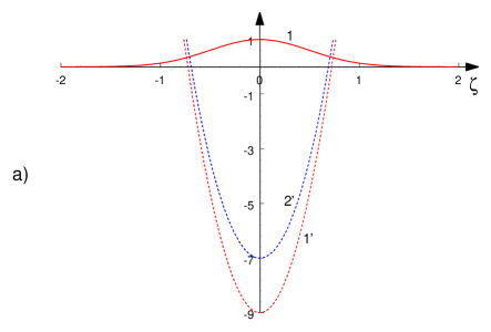
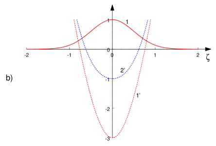
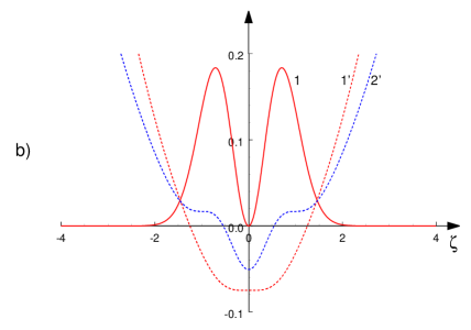
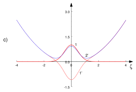
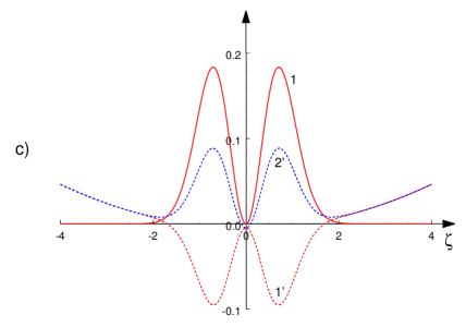
FIG. 11	FIG. 12

Figure 11: Normalized Gaussian solution (25) in terms of $F^{2}(\zeta)$ (solid curve $1$) and corresponding normalized potentials $v_{e}(\zeta)$ (broken curves $1^{\prime}$ and $2^{\prime}$, pertaining to $\sigma=1$ and $\sigma=-1$, respectively), as functions of normalized coordinate $\zeta$. Panels a), b), and c) were generated for $S=0.5$, $S=1$, and $S=5$, respectively. Note that the plots are shown on different scales.

Figure 12: The same as in Fig. 12 but for the derivative-Gaussian solution (26). The corresponding potentials are additionally reduced by the factor $K$: $v_{e}(\zeta)/K$, where $K$ is different in each panel. Panel a): $S=1$, $K=100$ for $\sigma=\pm 1$; panel b): $S=2$, $K=20$ for $\sigma=1$ and $S=2e$, $K=4$ for $\sigma=-1$; and panel c): $S=25$, $K=2$ for $\sigma=\pm 1$.

where $A$, $B$ and $l_{1,2}$ are arbitrary constants. This function resembles, in particular, a numerical solution which was found in Ref. [5] (see also review [6]) for the OL potential. Function (27) and the corresponding potential, as given by Eq. (24), can be presented in the following dimensionless form:

$$F(\zeta)=\exp{(-\zeta^{2})}+b\cos\left({\kappa\zeta}\right)\exp{[-(\varepsilon\zeta)^{2}]},$$ (28)

$$v_{e}(\zeta) = \frac{4}{S^{2}}\frac{\zeta^{2}-\frac{1}{2}+b\left[\left(\varepsilon^{4}\zeta^{2}-\frac{\varepsilon^{2}}{2}-\frac{\kappa^{2}}{4}\right)\cos\left({\kappa\zeta}\right)+\varepsilon^{2}\kappa\zeta\sin\left({\kappa\zeta}\right)\right]\exp{[-(\varepsilon^{2}-1)\zeta^{2}]}}{1+b\cos\left({\kappa\zeta}\right)\exp{[-(\varepsilon^{2}-1)\zeta^{2}]}}{}$$ (29)

$${}{}-\sigma\exp{(-2\zeta^{2})}\left\{1+b\cos\left({\kappa\zeta}\right)\exp{\left[-(\varepsilon^{2}-1)\zeta^{2}\right]}\right\}^{2}-M,$$

where $F(\zeta)=\varphi(\zeta)/A$, $v_{e}(\xi)=u(\xi)/A^{2}$, and $\zeta=\xi/l_{1}$, $b=B/A$, $\kappa=kl_{1}$, $\varepsilon=l_{1}/l_{2}$, $S=Al_{1}$, $M=-\mu/A^{2}$. Varying parameters $S$, $M$, $\kappa$, $b$ and $\varepsilon$, one can obtain a wide class of solutions. The corresponding potentials asymptotically approach the parabolic shape at large $|\xi|$, featuring a complex oscillatory shape at the center. Solution (28), $F^{2}(\zeta)$ and the corresponding potential (29) are shown in Fig. 13 for both signs of $\sigma$.

The stability of the Gaussian-type solutions. Stability of all solutions presented in this section was tested via simulations of Eq. (1). The results are summarized as follows.

(1) In the case of the repulsive nonlinearity, $\sigma=1$, the Gaussian solution with potential (25) is stable for all values of $S$. It is stable too in the case of $\sigma=-1$ (the attractive nonlinearity) if the corresponding potential features the single-well shape (such as shown in Figs. 12a and 9b), i.e. $S\leq S_{\mathrm{thr}}\equiv\sqrt{2}$, see above. However, in the model with the attractive nonlinearity, the solution naturally becomes unstable when the single-well potential transforms into the double-well potential, i.e. when $S>\sqrt{2}$ (see line $2^{\prime}$ in Fig. 12c). In the latter case, the solution preserves its shape until $t\lesssim 20$, and then spontaneously splits into two pulses which quasi-regularly oscillate relative to each other.

(2) The derivative-Gaussian solution with potential (26) is stable in both cases of $\sigma=\pm 1$, provided that the underlying potential keeps the single-well shape, i.e. until $S\leq S^{+}_{\mathrm{thr}}\equiv 2$ for $\sigma=+1$ and $S\leq S^{-}_{\mathrm{thr}}\equiv 2e$ for $\sigma=-1$ (see Figs. 12a and 12b). At greater values of $S$, the solutions in the double-well potential (see Fig. 12c) are unstable, for either sign of $\sigma$. However, manifestations of the instability are different for $\sigma=+1$ and $\sigma=-1$. In the former case, the initial distribution was preserved in a quasi-stable state until $t\approx 40$. Then, the profile of $|\varphi(\xi)|$ became asymmetric, with one maximum (for instance, the right one, as in Fig. 14a) being greater than the other. After reaching a well-pronounced asymmetric shape, the process reverted, making the left maximum greater than the right one. This process repeated persistently, so that the initial soliton

Figure 13: Squared solution (28), $F^{2}(\zeta)$, (panel a) and the corresponding potential (29) (reduced by the factor of $10$) for $\sigma=1$ (panel b) and $\sigma=-1$ (panel c) as functions of $\zeta$. Parameters are $S=5$, $M=0$, $\kappa=40$, $b=0.25$, $\varepsilon=2$.

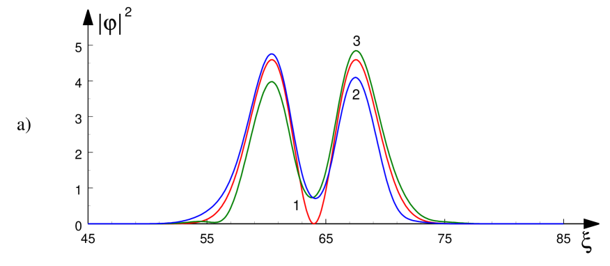
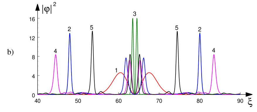
Figure 14: The spatial profile of $|\varphi|^{2}$ at different times, for the derivative-Gaussian initial configuration with $S=25$ (the size of the computation domain is $L=128$). In panel (a) pertaining to the case of $\sigma=1$ lines 1, 2 and 3 correspond, respectively, to $t=0,$ 50 and 60. In panel (b) pertaining to the case of $\sigma=-1$ lines 1, 2, 3, 4 and 5 correspond, respectively, to $t=0,$ 1, 2, 3, and 4 (note that there are two pulses of smaller amplitudes near the center at $t=1,$ 3 and 4).

was eventually transformed into an immobile breather consisting of two non-stationary pulses which oscillate in time quasi-randomly due to the energy exchange between them and, apparently, due to their interaction with a linear wave-train shed off by the pulses. It is worthy to note that the instability of the odd mode trapped in the double-well potential shown, for instance, in Fig. 12c, sets in via the breaking of the skew symmetry of this mode, in agreement with the general principle that the repulsive nonlinearity gives rise to the symmetry breaking of odd modes trapped in double-well potentials [11].

In the case of $\sigma=-1$, the character of instability observed at $S>S^{-}_{\mathrm{thr}}$ is different. For instance, at $S=25$ the solution became unstable at $t\approx 5$, splitting into four pulses and a small-amplitude wave train (see line 2 in Fig. 14). Two of those four pulses moved to the left and two others – to the right. After passing some distance, these pulses bounced back from the parabolic potential, moved back towards the center, and formed two very narrow and closely located spikes (see line 3 in Fig. 14). Such cycles of the splitting and partial recombination with the pulse compression in the vicinity of the center repeated indefinitely long. Thus, some type of a double breather is formed in this case too.

(3) The comb-top Gaussian solution with potential (29) is stable in the model with the repulsive nonlinearity, $\sigma=1$ (we did not explore the stability of this solution in a wide range of parameters; here we report an example for $b=1/4$, $\varepsilon=2$, $\kappa=40$, $M=0$, and $S=5$). Namely, if external perturbations were added to the solution, e.g., $A$ in Eq. (27) was taken $10\%$ smaller or grater against its stationary value, the evolution lead to time variations of $|\varphi|$ within the same $10\%$ range, similar to what was reported in item (1) above for the Gaussian initial distribution.

In the case of the attractive nonlinearity, $\sigma=-1$, with the same set of parameters as above, the initial real wave function (27) was quickly, within $t\approx 5$, transformed into a complex one, with a subsequent quasi-random energy exchange between the real and imaginary parts. At the initial stage of the evolution, the central part of the solution would transform into a very narrow large-amplitude pulse, with two side wings represented by small-amplitude wide pulses. Then, the central pulse would oscillate in time quasi-randomly.

3 Exact solutions for the two-dimensional stationary Gross–Pitaevskii equation

In this section we proceed to the consideration of the 2D version of the stationary GPE, taken in the dimensionless form similar to Eq. (5), with spatial coordinates $\xi$ and $\eta$:

$$\varphi_{\xi\xi}+\varphi_{\eta\eta}=\left[u(\xi,\eta)-\mu\right]\varphi+\sigma|\varphi|\,^{2}\varphi.$$ (30)

The approach similar to that which was developed in subsection 2.5 can be employed to construct an appropriate 2D potential on the basis of a given solution. From Eq. (30) one formally deduces

$$u(\xi,\eta)=\left(\varphi_{\xi\xi}+\varphi_{\eta\eta}\right)/\varphi-\sigma\varphi\,^{2}+\mu.$$ (31)

Examples presented below aim to demonstrate solutions which may be useful to physical applications.

The Kadomtsev–Petviashvili lump soliton. As the first trial function, we take an anisotropic 2D weakly localized ansatz known as the lump solution to the KP1 equation [28]:

$$\Phi(\xi,\eta)=12A\frac{3-(\xi/a)^{2}+(\eta/b)^{2}}{\left[3+(\xi/a)^{2}+(\eta/b)^{2}\right]^{2}}.$$ (32)

Substituting it as $\varphi$ into Eq. (31), one obtains the corresponding potential,

$$v_{e}(\overline{\xi},\overline{\eta})=-\frac{6}{S^{2}}\frac{P_{4}(\overline{\xi},\overline{\eta})}{(3+\overline{\xi}^{2}+\overline{\eta}^{2})^{2}(3-\overline{\xi}^{2}+\overline{\eta}^{2})}-144\sigma\frac{\left(3-\overline{\xi}^{2}+\overline{\eta}^{2}\right)^{2}}{\left(3+\overline{\xi}^{2}+\overline{\eta}^{2}\right)^{4}}+M,$$ (33)

where $v_{e}=u/A^{2}$, $\overline{\xi}=\xi/a$, $\overline{\eta}=\eta/b$, $S=Ab$, $\beta=b/a$, $M=\mu/A^{2}$, and $P_{4}(\overline{\xi},\overline{\eta})=(\beta^{2}-1)(\overline{\xi}^{4}+\overline{\eta}^{4})+6(1-\beta^{2})(\overline{\xi}\overline{\eta})^{2}-2(\overline{\xi}^{2}+\overline{\eta}^{2})-9\beta^{2}(2\overline{\xi}^{2}+\overline{\eta}^{2})+3(1+3\beta^{2})$. In the particular case of $\beta=1$ ($a=b$), Eq. (33) simplifies to

$$v_{e}(\overline{\xi},\overline{\eta})=-144\frac{2(3-5\overline{\xi}^{2}+\overline{\eta}^{2})+\sigma(3-\overline{\xi}^{2}+\overline{\eta}^{2})^{2}}{(3+\overline{\xi}^{2}+\overline{\eta}^{2})^{4}}+M.$$ (34)

Both expressions (33) and (34) correspond to anisotropic 2D trapping potentials. Figure 15a shows a 3D view of lump solution (32) for $a=b$, and Figs. 15b,c display the corresponding potential (34) for $\sigma=\pm 1$. In the case $\sigma=-1$, the potential represents a 2D hump, i.e. it is repulsive, hence the corresponding solution (32) is apparently unstable.

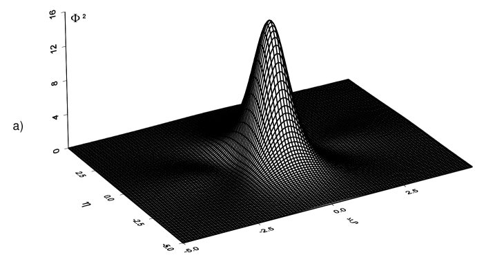
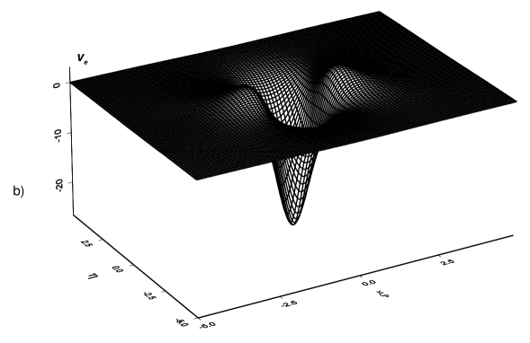
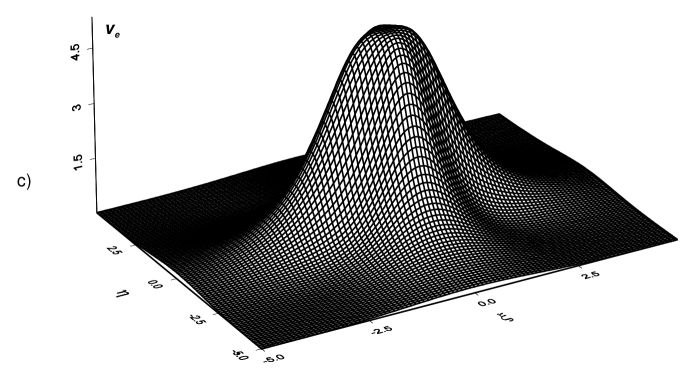
Figure 15: (a) Lump solution (32) shown in terms of $\left[\Phi\left(\xi,\eta\right)/A\right]^{2}$ for $a=b$  and $M=0$; and the corresponding potential (34) for $\sigma=1$ (b) and $\sigma=-1$ (c).

2D Gaussian trial function. Another natural example in the 2D case is provided by the solution ansatz in the form of an axisymmetric Gaussian, $\Phi(r)=A\exp{(-r^{2}/l^{2})}$, where $r^{2}=\xi^{2}+\eta^{2}$. From Eq. (30) we deduce the potential in the dimensionless form:

$$v_{e}(\rho)=\frac{4}{S^{2}}\left(\rho^{2}-1\right)-\sigma\exp{(-2\rho^{2})}+M,$$ (35)

where $v_{e}=u/A^{2}$, $\rho=r/l$, $S=Al$ and $M=\mu/A^{2}$ (the same particular solution was recently obtained in Ref. [36] in a different way, and its stability has been established in direct simulation). The principal cross-sections of the squared Gaussian solution and the corresponding potentials for $\sigma=\pm 1$ are shown in Fig. 16 for three values of $S$. In the case of the attractive nonlinearity, $\sigma=-1$, potential function $v_{e}$ may feature a local maximum at the center, which appears at $S>\sqrt{2}$ (see Fig. 16c).

Other examples represent 2D patterns of a different type, namely, vortices. First we present the unitary vortex, with topological charge $J=1$ (it may be treated as a 2D counterpart of the 1D derivative-Gaussian profile considered above): $\Phi(\xi,\eta)=A(\xi+i\eta)\exp{(-r^{2}/l^{2})}$, where $r=\sqrt{\xi^{2}+\eta^{2}}$. For the complex solution it is convenient to cast the stationary GPE (30) into the following real form: $(1/2)\left[\Delta\left(|\varphi|^{2}\right)-2|\nabla\varphi|^{2}\right]-\sigma|\varphi|^{4}=[u(\xi,\eta)-\mu]|\varphi|^{2},$ where $\Delta$ is the 2D Laplacian. From this equation, one can deduce the potential:

$$u(\xi,\eta)=\frac{\Delta|\varphi|^{2}-2|\nabla\varphi|^{2}}{2|\varphi|^{2}}-\sigma|\varphi|^{2}+\mu.$$ (36)

Substituting here the wave function of the vortex, the potential can be obtained in the explicit form [cf. Eq. (26)]:

$$v_{e}(\rho)=\left(4/S^{2}\right)\left(\rho^{2}-2\right)-\sigma\rho^{2}\exp{(-2\rho^{2})}+M,$$ (37)

where $v_{e}=u/(Al)^{2}$, $\rho=r/l$, $S=Al^{2}$, and $M=\mu/(Al)^{2}$. Principal cross-sections of the solution for $|\Phi(\rho)|^{2}$ and the corresponding potentials for $\sigma=\pm 1$ are shown in Fig. 18, for three values of $S$.

The double vortex. We have also considered the trial solution in the form of the vortex with $J=2$, viz., $\Phi(\xi,\eta)=A(x+iy)^{2}\exp{(-r^{2}/l^{2})}$. One can readily deduce from Eq. (36) the potential supporting this solution:

$$v_{e}(\rho)=\left(4/S^{2}\right)\left(\rho^{2}-3\right)-\sigma\rho^{4}\exp{(-2\rho^{2})}+M,$$ (38)

where $v_{e}=u/(Al^{2})^{2}$, $\rho=r/l$, $S=Al^{3}$, and $M=\mu/(Al^{2})^{2}$. Principal cross-sections of the solution for $|\Phi(\rho)|^{2}$ and the corresponding potentials for $\sigma=\pm 1$ are shown in Fig. 18 for the same three values of $S$ as in Fig. 18.

4 Exact solutions for the three-dimensional stationary Gross–Pitaevskii equation

In this section we briefly demonstrate the applicability of the above method to the 3D case (with the usual Laplacian corresponding to the GPE). The scaled 3D version of the stationary GPE is

$$\frac{\partial\,^{2}\varphi}{\partial\xi\,^{2}}+\frac{\partial\,^{2}\varphi}{\partial\eta\,^{2}}+\frac{\partial\,^{2}\varphi}{\partial\zeta\,^{2}}=\left[u(\xi,\eta)+\mu\right]\varphi+\sigma|\varphi|\,^{2}\varphi,$$ (39)

where function $\varphi$ depends on three spatial coordinates – $\xi$, $\eta$, and $\zeta$. From Eq. (39) one can readily deduce the necessary potential:

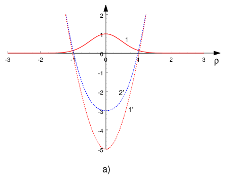
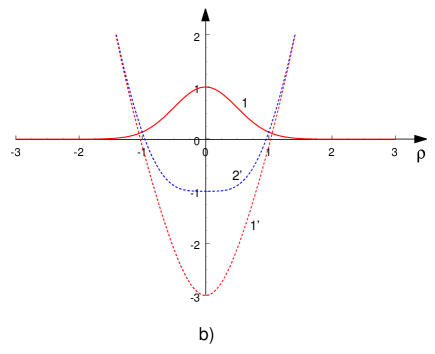
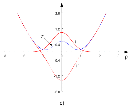
Figure 16: The radial distribution of density $|\varphi(\rho)|^{2}$ for the 2D Gaussian solution (lines $1$ in each panel) and the corresponding potentials (35) with $M=0$ for the repulsive ($\sigma=1$, lines $1^{\prime}$) and attractive ($\sigma=-1$, lines $2^{\prime}$) nonlinearities: a) $S=1$, b) $S=\sqrt{2}$, c) $S=3$.

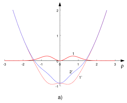
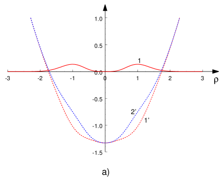
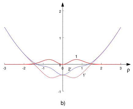
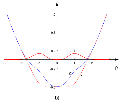
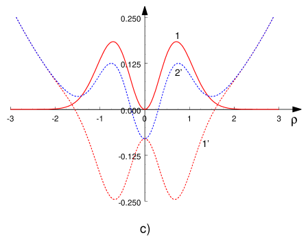
FIG. 17	FIG. 18

Figure 17: The radial distribution of density $|\varphi(\rho)|^{2}$ in the unitary vortex solution (lines $1$), and the corresponding potentials (37) with $M=0$ for the repulsive ($\sigma=1$, lines $1^{\prime}$) and attractive ($\sigma=-1$, lines $2^{\prime}$) nonlinearity. a) $S=3$, b) $S=4.5$, c) $S=10$.

Figure 18: The radial distribution of density $|\varphi(\rho)|^{2}$ for the double vortex (lines $1$), and the corresponding potentials (38) with $M=0$ for the repulsive ($\sigma=1$, lines $1^{\prime}$) and attractive ($\sigma=-1$, lines $2^{\prime}$) nonlinearities. a) $S=3$, b) $S=4.5$, c) $S=10$.

$$u(\xi,\eta)=\frac{1}{\varphi}\left(\frac{\partial\,^{2}\varphi}{\partial\xi\,^{2}}+\frac{\partial\,^{2}\varphi}{\partial\eta\,^{2}}+\frac{\partial\,^{2}\varphi}{\partial\zeta\,^{2}}\right)-\sigma\varphi\,^{2}-\mu.$$ (40)

We here present an example of the 3D trial function in the form of the spherically symmetric Gaussian, $\Phi(r)=A\exp{(-r^{2}/l^{2})}$, where $r^{2}=\xi^{2}+\eta^{2}+\zeta^{2}$. The corresponding potential can be found from Eq. (39):

$$v_{e}(\rho)=\frac{4}{S^{2}}\left(\rho^{2}-\frac{3}{2}\right)-\sigma\exp{(-2\rho^{2})}-M,$$ (41)

where $v_{e}=u/A^{2}$, $\rho=r/l$, $S=Al$, and $M=\mu/A^{2}$. The plot of the potential, $v_{e}(\rho)$, is similar to that shown in Fig. 16. In a similar way, one can readily construct potentials for many other cases including 3D generalizations of the examples presented above in terms of the 2D geometry.

5 Conclusions

We have demonstrated that numerous exact 1D stationary solutions to the GPE (Gross–Pitaevskii equation) may be constructed with the help of the Kondrat’iev–Miller method [30]. Within the framework of this method, the corresponding potential function in the GPE is proportional to stationary solution $\varphi(\xi)$, which, in turn, was taken as a solution to the stationary GE (Gardner equation). The stability of the 1D solutions was tested through direct simulations of the time-dependent GPE. It was found that some solitary-type solutions are stable – in particular, those corresponding to the solution of the GE in the form of the “fat” (table-top) soliton, which is given by Eq. (10), in the case of the repulsive nonlinearity. A stable soliton solution in the case of the attractive nonlinearity was also found, viz., the exponentially localized solution given by expression (16).

Further, we have proposed an “inverse method” for the GPE, as a way to construct appropriate potentials for a given distribution of the wave function. It was demonstrated that this method helps to produce many solutions in 1D and 2D settings. The stability of all the so found 1D solutions has been tested in direct simulations. The 1D and 2D potentials constructed here as supports for basic natural types of the localized matter-wave distributions are fairly simple, and may be realized in the experiment by means of currently available techniques, based on the design of appropriate magnetic and optical traps for the BEC.

The numerical scheme employed here for the simulations of the time-dependent GPE in 1D is based on the Yunakovsky’s method of the operator exponential, which has been used in many previous works (see, e.g., Ref. [29]). The method is also efficient in obtaining solutions to NLSE and GPE in the space of any dimension. It is briefly described in Appendix.

In addition to testing the stability of the 2D localized solutions, another remaining issue is to check whether the specially designed potentials which support 1D and 2D solutions, as ground states, may also sustain higher-order bound states in the respective nonlinear Further, the inverse method can be readily extended to the 3D settings. Some results have been already obtained in this direction, to be reported elsewhere. Finally, it may be quite interesting to apply both the GE and the inverse method to constructing exact solutions for dark solitons in 1D and circular dark solitons in 2D [37], in the case of the modulationally stable background. These generalizations will be also reported elsewhere.

Acknowledgements. This work was partially supported by the German–Israel Foundation through the grant No. 149/2006. Y.S. appreciates hospitality of the Faculty of Engineering at the Tel Aviv University during his visit in 2009.

6 Appendix: The numerical algorithm for simulations of the Gross-Pitaevskii equation

In this Appendix we describe a numerical algorithm based on the method originally developed by Yunakovsky for the numerical solution of the NLSE [29]. The method works equally well in 1D, 2D and 3D settings. Below give a brief account of the method in the application to the 1D case, it generalization for 2D and 3D settings being straightforward.

One starts by the application of the Fourier transform to variable $\xi$ in Eq. (1):

$$i\frac{\partial\widetilde{\varphi}}{\partial t}=k^{2}\widetilde{\varphi}+\hat{F}\left\{[u(\xi)+\mu]\varphi\right\}+\sigma\hat{F}\left\{|\varphi|^{2}\varphi\right\},$$ (42)

where $k$ is the respective wavenumber, and the tilde stands for the Fourier image, which is generated by the Fourier-transform operator $\hat{F}$. Next, we introduce a new function, $u(k,t)=\widetilde{\varphi}(k,t)\exp{(ik^{2}t)}$, and rewrite Eq. (42) accordingly:

$$i\frac{\partial u}{\partial t}=\hat{F}\left\{\left[U_{\mu}(\xi)+\sigma|\varphi|^{2}\right]\varphi\right\}\exp{(ik^{2}t)},$$ (43)

where $U_{\mu}(\xi)\equiv u(\xi)+\mu$. This equation may be formally integrated in $t$, yielding, in terms of $\varphi$,

$$\widetilde{\varphi}(k,t)=\widetilde{\varphi}(k,0)\exp{(-ik^{2}t)}-i\int\limits_{0}^{t}\hat{F}\left\{\left[U_{\mu}(\xi)+\sigma|\varphi|^{2}\right]\varphi\right\}\exp{[-ik^{2}(t-\tau)]}\,d\tau.$$ (44)

The integral on the right-hand side can be approximately calculated, over a small time interval, with the help of the trapezoidal rule. The result, valid up to $O(t^{3})$, is

$$\widetilde{\varphi}(k,t)=\widetilde{\varphi}_{0}\exp{(-ik^{2}t)}-(it/2){}{}$$

$$\times\left[\hat{F}\left\{\left[U_{\mu}(\xi)+\sigma|\varphi_{0}|^{2}\right]\varphi_{0}\right\}\exp{(-ik^{2}t)}+\hat{F}\left\{\left[U_{\mu}(\xi)+\sigma|\varphi|^{2}\right]\varphi\right\}\right].$$ (45)

Next, we collect on the left-hand side those terms which depend on the current time, and leave on the right-hand side the terms which depend on initial conditions:

$$\widetilde{\varphi}(k,t)+\frac{it}{2}\hat{F}\left\{\left[U_{\mu}(\xi)+\sigma|\varphi|^{2}\right]\varphi\right\}=$$

$$\left(\widetilde{\varphi}_{0}-\frac{it}{2}\hat{F}\left\{\left[U_{\mu}(\xi)+\sigma|\varphi_{0}|^{2}\right]\varphi_{0}\right\}\right)\exp{(-ik^{2}t)}.$$ (46)

By applying the inverse Fourier transform, $\hat{F}^{-1}$, to Eq. (LABEL:Collection), one obtains

$$\left\{1+\frac{it}{2}\left[U_{\mu}(\xi)+\sigma|\varphi(\xi,t)|^{2}\right]\right\}\varphi(\xi,t)$$ (47)

$$= \hat{F}^{-1}\left\{\left[\widetilde{\varphi}_{0}(k)-\frac{it}{2}\hat{F}\left\{\left[U_{\mu}(\xi)+\sigma|\varphi_{0}|^{2}\right]\varphi_{0}\right\}\right]\exp{(-ik^{2}t)}\right\}\equiv B(\xi,t).$$

Function $B(\xi,t)$ produced by Eq. (47) is an explicit result obtained from the given initial condition, $\varphi_{0}(k)\equiv\widetilde{\varphi}(\xi,0)$. Then, function $\varphi(\xi,t)$ can be formally found from Eq. (47):

$$\varphi(\xi,t)=\frac{B(\xi,t)}{1+(it/2)\left[U_{\mu}(\xi)+\sigma|\varphi(\xi,t)|^{2}\right]}.$$ (48)

To make this formula practical, one needs to define $|\varphi(\xi,t)|^{2}$ in the denominator of Eq. (48). To do that, take Eq. (47) and multiply it by the complex conjugate counterpart, which yields

$$\left\{1+\left(t^{2}/4\right)\left[U_{\mu}(\xi)+\sigma|\varphi|^{2}\right]^{2}\right\}|\varphi(\xi,t)|^{2}=|B(\xi,t)|^{2}.$$ (49)

Thus, denoting $z\equiv|\varphi(\xi,t)|^{2}$ and taking into account that $\sigma^{2}=1$, we obtain a cubic equation for $z$:

$$z^{3}+2\sigma U_{\mu}(\xi)z^{2}+\left[\left(4/t^{2}\right)+U_{\mu}(\xi)\right]z-\left(4/t^{2}\right)|B(\xi,t)|^{2}=0.$$ (50)

The cubic equation can be solved analytically, in principle. Its single real root (two others are complex) can be found by means of symbolic calculations realized by means of software such as Maple:

$$z=\frac{2}{3}\left[\mathrm{Root3}-\frac{1/t^{2}+U_{\mu}(\xi)/4-U_{\mu}^{2}(\xi)/3}{\mathrm{Root3}}-\sigma U_{\mu}(\xi)\right],$$ (51)

where we define

$$\mathrm{Root3} = \left\{\frac{9}{8}\sigma U_{\mu}(\xi)\left[\frac{4}{t^{2}}+U_{\mu}(\xi)\right]+\frac{27}{4t^{2}}|B(\xi,t)|^{2}-\sigma U_{\mu}^{3}(\xi)+\frac{3}{8t^{3}}\sqrt{X}\right\}^{1/3},$$

$$X = 3\left\{\left[1-U_{\mu}(\xi)\right]U_{\mu}^{3}(\xi)t^{6}+4\left[3-2U_{\mu}(\xi)+\sigma\left(9-8U_{\mu}(\xi)\right)|B(\xi,t)|^{2}\right]U_{\mu}^{2}(\xi)t^{4}+{}\right.$$ (52)

$$\left.\left[48U_{\mu}(\xi)+\left(144\sigma U_{\mu}(\xi)+108\right)|B(\xi,t)|^{2}-168\sigma U_{\mu}^{2}(\xi)\right]t^{2}+64\right\}.$$

Once root $z$ was found, it can be substituted into the denominator of Eq. (48); then, function $\varphi(\xi,t)$ is completely determined at time $t$. After that, the procedure may be repeated for the next time step.

References

- [1] L. P. Pitaevskii and S. Stringari, Bose–Einstein Condensation. (Clarendon, Oxford, 2003).
- [2] M. M. Cerimele, M. L. Chiofalo, F. Pistella, S. Succi, and M. P. Tosi, Phys. Rev. E 62, 1382 (2000).
- [3] S. K. Adhikari and P. Muruganandam, J. Phys. B: At. Mol. Opt. Phys. 35, 2831 (2002); P. Muruganandam and S. K. Adhikari, ibid. 36, 2501 (2003); W. Z. Bao, D. Jaksch, and P. A. Markowich, J. Comp. Phys. 187, (2003).
- [4] S. K. Adhikari, Phys. Rev. E 65, 016703 (2002).
- [5] M. L. Chiofalo, S. Succi, and M. P. Tosi, Phys. Rev. E 62, 7438 (2000); W. Z. Bao and Q. Du, SIAM J. Scient. Comp. 25, 1674 (2004).
- [6] A. Minguzzi, S. Succi, F. Toschi, M. P. Tosi, and P. Vignolo, Phys. Rep. 395, 223 (2004).
- [7] V. M. Pérez-García, H. Michinel, J. I. Cirac, M. Lewenstein, and P. Zoller, Phys. Rev. A 56, 1424 (1997); A. L. Fetter, J. Low Temp. Phys. 106, 643 (1997); B. A. Malomed, in Progr. Optics, ed. by E. Wolf, vol. 43, p. 71 (North Holland, Amsterdam, 2002); S. K. Adhikari and B. A. Malomed, Phys. Rev. A 77, 023607 (2008).
- [8] L. Salasnich, A. Parola, and L. Reatto, Phys. Rev. A 65, 043614 (2002); L. Salasnich and B. A. Malomed, ibid. 74, 053610 (2006); A. Muñoz Mateo and V. Delgado, ibid. 77, 013617 (2008).
- [9] A. Trombettoni and A. Smerzi, Phys. Rev. Lett. 86, 2353 (2001); F. Kh. Abdullaev, B. B. Baizakov, S. A. Darmanyan, V. V. Konotop, and M. Salerno, Phys. Rev. A 64, 043606 (2001); G. L. Alfimov, P. G. Kevrekidis, V. V. Konotop, and M. Salerno, Phys. Rev. E 66, 046608 (2002); R. Carretero-González and K. Promislow, Phys. Rev. A 66, 033610 (2002); M. A. Porter, R. Carretero-González, P. G. Kevrekidis, and B. A. Malomed, Chaos 15, 015115 (2005); A. Maluckov, L. Hadžievski, B. A. Malomed, and L. Salasnich, Phys. Rev. A 78, 013616 (2008).
- [10] F. Dalfovo, C. Minniti, S. Stringari, L. Pitaevskii, Phys. Lett. A 227, 259 (1997).
- [11] E. A. Ostrovskaya, Y. S. Kivshar, M. Lisak, B. Hall, F. Cattani, and D. Anderson, Phys. Rev. A 61, 031601(2000); R. D’Agosta, B. A. Malomed, C. Presilla, Phys. Lett. A 275, 424 (2000); R. K. Jackson and M. I. Weinstein, J. Stat. Phys. 116, 881 (2004); V. S. Shchesnovich, B. A. Malomed, and R. A. Kraenkel, Physica D 188, 213 (2004); D. Ananikian and T. Bergeman, Phys. Rev. A 73, 013604 (2006); C. Wang, P. G. Kevrekidis, N. Whitaker and B. A. Malomed, Physica D 327, 2922 (2008); E. W. Kirr, P. G. Kevrekidis, E. Shlizerman, and M. I. Weinstein, SIAM J. Math. Anal. 40, 566 (2008).
- [12] F. Kh. Abdullaev, A. M. Kamchatnov, V. V. Konotop, and V. A. Brazhnyi, Phys. Rev. Lett. 90, 230402 (2003); D. E. Pelinovsky, P. G. Kevrekidis, and D. J. Frantzeskakis, Phys. Rev. Lett. 91, 240201 (2003); F. Kh. Abdullaev and J. Garnier, Phys. Rev. A 70, 053604 (2004); D. E. Pelinovsky, P. G. Kevrekidis, D. J. Frantzeskakis, and V. Zharnitsky, Phys. Rev. E 70, 047604 (2004).
- [13] Yu. S. Kivshar and B. A. Malomed, Rev. Mod. Phys. 61, 763 (1989).
- [14] P. G. Kevrekidis, G. Theocharis, D. J. Frantzeskakis and B. A. Malomed, Phys. Rev. Lett. 90, 230401 (2003); L. D. Carr and J. Brand, ibid. 92, 040401 (2004); V. P. Barros, M. Brtka, A. Gammal, and F. Kh. Abdullaev, J. Phys. B: At. Mol. Opt. Phys. 38, 4111 (2005).
- [15] R. Carretero-González, D. J. Frantzeskakis, and P. G. Kevrekidis, Nonlinearity 21, R139 (2008).
- [16] J. Belmonte-Beitia, V. V. Konotop, V. M. Pérez-García, and V. E. Vekslerchik, Chaos, Solitons & Fractals 41, 1158 (2009).
- [17] L. D. Carr, C. W. Clark, and W. P. Reinhardt, Phys. Rev. A 62, 063610 (2000); J. C. Bronski, L. D. Carr, B. Deconinck, J. N. Kutz, and K. Promislow, Phys. Rev. E 63, 036612 (2001).
- [18] L. D. Carr, C. W. Clark, and W. P. Reinhardt, Phys. Rev. A 62, 063611 (2000); J. C. Bronski, L. D. Carr, R. Carretero-González, B. Deconinck, J. N. Kutz, and K. Promislow, Phys. Rev. E 64, 056615 (2001).
- [19] B. T. Seaman, L. D. Carr, and M. J. Holland, Phys. Rev. A 72, 033602 (2005).
- [20] G. A. El, A. Gammal, and A. M. Kamchatnov, Phys. Rev. Lett. 97, 180405 (2006).
- [21] D. Witthaut, S. Mossmann, and H. J. Korsch, J. Phys. A; Math. Gen. 38, 1777 (2005).
- [22] T. Mayteevarunyoo, B. A. Malomed, and G. Dong, Phys. Rev. A 78, 053601 (2008).
- [23] Y. S. Kivshar and G. P. Agrawal, Optical Solitons (Academic Press: San Diego, 2003).
- [24] L. Fallani, C. Fort, and M. Inguscio, Rivista Nuovo Cim. 28, 1 (2005).
- [25] K. Henderson, C. Ryu, C. MacCormick, and M. G.I Boshier, New J. Phys. 11, 043030 (2009).
- [26] S. Flach, Y. Zolotaryuk, and K. Kladko, Phys. Rev. E 59, 6105 (1999); I. V. Barashenkov, O. F. Oxtoby, and D. E. Pelinovsky, ibid. E 72, 035602 (2005); D. E. Pelinovsky, Nonlinearity 19, 2695 (2006); S. V. Dmitriev, P. G. Kevrekidis, A. A. Sukhorukov, N. Yoshikawa, and S. Takeno, Phys. Lett. A 356, 324 (2006).
- [27] N. K. Efremidis, G. A. Siviloglou, and D. N. Christodoulides, Phys. Lett. A 373, 4073 (2009).
- [28] M. J. Ablowitz, and H. Segur, Solitons and the Inverse Scattering Transform (SIAM, Philadelphia, 1981).
- [29] A. D. Yunakovsky, Simulation of the Nonlinear Schrödinger Equation. (IPF RAN, Nizhny Novgorod, IPF RAN, 1995) (in Russian); G. M. Fraiman, E. M. Sher, A. D. Yunakovsky, and W. Laedke, Physica D 87, 325(1995); Ya. L. Bogomolov and A. D. Yunakovsky, Split-step Fourier method for nonlinear Schrödinger equation, in: Proceedings of the International Conference, “Days on Diffraction”, p. 34(2006) (DOI: 10.1109/DD.2006.348170; see also: http://www.mendeley.com/c/81983606/Bogomolov-2006-Splitstep-Fourier-method-for-nonlinear-Schrödinger-equation/)
- [30] I. G. Kondrat’ev and M. A. Miller, Izv. VUZov, Radiofizika IX, 910 (1966) [in Russian; English translation: Sov. J. Radiophys. Quantum Electr. IX, 532 (1966)].
- [31] A. W. Snyder, D. J. Mitchell, L. Poladian, and F. Ladouceur, Opt. Lett. 16, 21 (1991).
- [32] J. W. Miles, Tellus 33, 397 (1981); T. R. Marchant, and N. F. Smyth, IMA J. Appl. Math. 56, 157 (1996); A. V. Slyunyaev, ZhETF 119, 606 (2001) [in Russian; English translation: JETP 92(3) 529 (2001)]; R. Grimshaw, D. Pelinovsky, E. Pelinovsky, and A. Slyunyaev, Chaos 12 1070 (2002).
- [33] L. A. Ostrovsky, and Y. A. Stepanyants, Chaos, 15, 037111 (2005). J. Apel, L. A. Ostrovsky, Y. A. Stepanyants, and J. F. Lynch, J. Acoust. Soc. Am. 121, 695 (2007).
- [34] D. E. Pelinovsky, and R. H. J. Grimshaw, Phys. Let. A. 229, 165 (1997); R. Grimshaw, A. Slunyaev, and E. Pelinovsky, Chaos, (2010) – to be published.
- [35] A. V. Slyunyaev and E. N. Pelinovskii, ZhETF 116, 318 (1999) [in Russian; English translation: JETP 89(1) 173 (1999)].
- [36] Y. Wang, and R. Hao, Opt. Commun. 282 3995 (2009).
- [37] G. Theocharis, D. J. Frantzeskakis, P. G. Kevrekidis, B. A. Malomed, and Y. S. Kivshar, Phys. Rev. Lett. 90, 120403 (2003).