Exponential Screening and
optimal rates of sparse estimation

Abstract

In high-dimensional linear regression, the goal pursued here is to estimate an unknown regression function using linear combinations of a suitable set of covariates. One of the key assumptions for the success of any statistical procedure in this setup is to assume that the linear combination is sparse in some sense, for example, that it involves only few covariates. We consider a general, non necessarily linear, regression with Gaussian noise and study a related question that is to find a linear combination of approximating functions, which is at the same time sparse and has small mean squared error (MSE). We introduce a new estimation procedure, called Exponential Screening that shows remarkable adaptation properties. It adapts to the linear combination that optimally balances MSE and sparsity, whether the latter is measured in terms of the number of non-zero entries in the combination ($\ell_{0}$ norm) or in terms of the global weight of the combination ($\ell_{1}$ norm). The power of this adaptation result is illustrated by showing that Exponential Screening solves optimally and simultaneously all the problems of aggregation in Gaussian regression that have been discussed in the literature. Moreover, we show that the performance of the Exponential Screening estimator cannot be improved in a minimax sense, even if the optimal sparsity is known in advance. The theoretical and numerical superiority of Exponential Screening compared to state-of-the-art sparse procedures is also discussed.

Mathematics Subject Classifications: Primary 62G08, Secondary 62G05, 62J05, 62C20, 62G20.

Key Words: High-dimensional regression, aggregation, adaptation, sparsity, sparsity oracle inequalities, minimax rates, Lasso, BIC.

1 Introduction

The theory of estimation in high-dimensional statistical models under the sparsity scenario has been considerably developed during the recent years. One of the main achievements was to derive sparsity oracle inequalities (SOI), i.e., bounds on the risk of various sparse estimation procedures in terms of the $\ell_{0}$ norm (number of non-zero components) of the estimated vectors or their approximations (see Bickel et al., 2009; Bunea et al., 2007a, b; Candes and Tao, 2007; Koltchinskii, 2008, 2009a, 2009b; van de Geer, 2008; Zhang and Huang, 2008; Zhang, 2009, and references therein). The main message of these results was to demonstrate that if the number of non-zero components of a high-dimensional target vector is small, then it can be reasonably well estimated even when the ambient dimension is larger than the sample size. However, there was relatively few discussion of the optimality of these bounds, mainly based on specific counter-examples or referring to the paper by Donoho and Johnstone (1994a), which treats the Gaussian sequence model. The latter approach is, in general, insufficient as we will show below. An interesting point related to the optimality issue is that some of the bounds in the papers mentioned above involve not only the $\ell_{0}$ norm but also the $\ell_{1}$ norm of the target vector, which is yet another characteristic of sparsity. Thus, a natural question is whether the $\ell_{1}$ norm plays an intrinsic role in the SOI or it appears there due to the techniques employed in the proof.

In this paper, considering the regression model with fixed design, we will show that the role of $\ell_{1}$ norm is indeed intrinsic. Once we have a “rather general SOI” in terms the $\ell_{0}$ norm, a SOI in terms of the $\ell_{1}$ norm follows as a consequence. This means that we can write the resulting bound with the rate which is equal to the minimum of the $\ell_{0}$ and $\ell_{1}$ rates (see Theorem 3.2). Unfortunately, the above mentioned “rather general SOI” is not available in the literature for the previously known sparse estimation procedures. We therefore suggest a new procedure called the Exponential Screening (es), which satisfies the desired bound. It is based on exponentially weighted aggregation of least squares estimators with suitably chosen prior. The idea of using exponentially weighted aggregation for sparse estimation is due to Dalalyan and Tsybakov (2007). Dalalyan and Tsybakov (2007, 2008, 2009, 2010) suggested several procedures of this kind based on continuous sparsity priors. Our approach is different because we use a discrete prior in the spirit of earlier work by George (1986a, b); Leung and Barron (2006); Giraud (2008). Unlike George (1986a, b); Leung and Barron (2006); Giraud (2008), we focus on high-dimensional models and treat explicitly the sparsity issue. Because of the high dimensionality of the problem, we need efficient computational algorithms, and therefore we suggest a version of the Metropolis-Hastings algorithm to approximate our estimators (subsection 7.1). Regarding the sparsity issue, we prove that our method benefits simultaneously from three types of sparsity. The first one is expressed by the small rank of the design matrix $\mathbf{X}$, the second by the small number of non-zero components of the target vector, and the third by its small $\ell_{1}$ norm. Finally, we mention that in a work parallel to ours, Alquier and Lounici (2010) consider exponentially weighted aggregates with priors involving both discrete and continuous components and suggest another version of the Metropolis-Hastings algorithm to compute them.

The contributions of this paper are the following:

• We propose the es estimator which benefits simultaneously from the above mentioned three types of sparsity. This follows from the oracle inequalities that we prove in Section 3. We also provide an efficient and fast algorithm to approximately compute the es estimator and show that it outperforms several other competitive estimators in a simulation study.

• We show that the es estimator attains the optimal rate of sparse estimation. To this end, we establish a minimax lower bound which coincides with the upper bound on the risk of the es estimator on the intersection of the $\ell_{0}$ and $\ell_{1}$ balls (Theorem 5.3).

• As a consequence, we find optimal rates of aggregation for the regression model with fixed design. We consider the five main types of aggregation, which are the linear, convex, model selection, subset selection and $D$-convex aggregation, cf. Nemirovski (2000); Tsybakov (2003); Bunea et al. (2007b); Lounici (2007). We show that the optimal rates are different from those for the regression model with random design established in Tsybakov (2003). Indeed, they turn out to be moderated by the rank of the regression matrix $\mathbf{X}$. The rates are faster for the smaller ranks. See Section 6.

This paper is organized as follows. After setting the problem and the notation in Section 2, we introduce the es estimator in Section 3 and prove that it satisfies a SOI with a remainder term obtained as the minimum of the $\ell_{0}$ and the $\ell_{1}$ rate. This result holds with no assumption on the design matrix ${\bf X}$, except for simple normalization. We put it into perspective in Section 4 where we compare it with weaker SOI for the bic and the Lasso estimators. In Sections 5.1 and 5.2 we discuss the optimality of SOI. In particular, Section 5.1 comments why a minimax result in Donoho and Johnstone (1994a) with normalization depending on the unknown parameter is not suitable to treat optimality. Instead, we propose to consider minimax optimality on the intersection of $\ell_{0}$ and $\ell_{1}$ balls. In Section 5.2 we prove the corresponding minimax lower bound for all estimators and show rate optimality of the es estimator in this sense. Section 6 discusses corollaries of our main results for the problem of aggregation; we show that the es estimator solves simultaneously and optimally the five problems of aggregation mentioned in (iii) above. Finally, Section 7 presents a simulation study demonstrating a good performance of the es estimator in numerical experiments.

2 Model and notation

Let $\mathcal{Z}:=\{(x_{1},Y_{1}),\ldots,(x_{n},Y_{n})\}$ be a collection of independent random couples such that $(x_{i},Y_{i})\in\mathcal{X}\times{\rm I}\kern-1.79993pt{\rm R}$, where $\mathcal{X}$ is an arbitrary set. Assume the regression model:

$$Y_{i}=\eta(x_{i})+\xi_{i},\ i=1,\ldots,n\,,$$

where $\eta:\mathcal{X}\to{\rm I}\kern-1.79993pt{\rm R}$ is the unknown regression function and the errors $\xi_{i}$ are independent Gaussian $\mathcal{N}(0,\sigma^{2})$. The covariates are deterministic elements $x_{1},\ldots,x_{n}$ of $\mathcal{X}$. Consider the equivalence relation $\sim$ on the space of functions $f:\mathcal{X}\to{\rm I}\kern-1.79993pt{\rm R}$ such that $f\sim g$ if and only if $f(x_{i})=g(x_{i})$ for all $i=1,\ldots,n$. Denote by $Q_{1:n}$ the quotient space associated to this equivalence relation and define the norm $\|\cdot\|$ by

$$\|f\|^{2}:=\frac{1}{n}\sum_{i=1}^{n}f^{2}(x_{i})\,,\quad f\in Q_{1:n}\,.$$

Notice that $\|\cdot\|$ is a norm on the quotient space but only a seminorm on the whole space of functions $f:\mathcal{X}\to{\rm I}\kern-1.79993pt{\rm R}$. Hereafter, we refer to it as a norm. We also define the associated inner product

$$\langle f,g\rangle:=\frac{1}{n}\sum_{i=1}^{n}f(x_{i})g(x_{i})\,.$$

Let $\mathcal{H}:=\{f_{1},\ldots,f_{M}\}$, be a dictionary of $M\geq 1$ given functions $f_{j}:\mathcal{X}\to{\rm I}\kern-1.79993pt{\rm R}$. We approximate the regression function $\eta$ by a linear combination ${\sf f}_{\theta}(x)=\sum_{j=1}^{M}\theta_{j}f_{j}(x)$ with weights $\theta=(\theta_{1},\dots,\theta_{M})$, where possibly $M\gg n$.

We denote by $\mathbf{X}$, the $n\times M$ design matrix with elements $\mathbf{X}_{i,j}=f_{j}(x_{i})$, $i=1,\ldots,n,j=1,\ldots,M$. We also introduce the column vectors ${\bf f}=(\eta(x_{1}),\dots,\eta(x_{n}))^{\top}$, $\mathbf{Y}=(Y_{1},\dots,Y_{n})^{\top}$ and $\xi=(\xi_{1},\dots,\xi_{n})^{\top}$. Let $|\cdot|_{p}$ denote the $\ell_{p}$ norm in ${\rm I}\kern-1.79993pt{\rm R}^{d}$ for $p,d\geq 1$ and $M(\theta)$ denote the $\ell_{0}$ norm of $\theta\in{\rm I}\kern-1.79993pt{\rm R}^{M}$, i.e., the number of non-zero elements of $\theta\in{\rm I}\kern-1.79993pt{\rm R}^{M}$. For two real numbers $a$ and $b$ we use the notation $a\wedge b:=\min(a,b)$, $a\vee b:=\max(a,b)$; we denote by $[a]$ the integer part of $a$ and by $\lceil a\rceil$ the smallest integer greater than or equal to $a$.

3 Sparsity pattern aggregation and Exponential Screening

A sparsity pattern is a binary vector ${\sf p}\in\mathcal{P}:=\{0,1\}^{M}$. The terminology comes from the fact that the coordinates of any such vectors can be interpreted as indicators of presence (${\sf p}_{j}=1$) or absence (${\sf p}_{j}=0$) of a given feature indexed by $j\in\{1,\ldots,M\}$. We denote by $|{\sf p}|$ the number of ones in the sparsity pattern ${\sf p}$ and by ${\rm I}\kern-1.79993pt{\rm R}^{\sf p}$ the space defined by

$${\rm I}\kern-1.79993pt{\rm R}^{\sf p}=\{\theta\cdot{\sf p}\,:\,\theta\in{\rm I}\kern-1.79993pt{\rm R}^{M}\}\subset{\rm I}\kern-1.79993pt{\rm R}^{M}\,,$$

where $\theta\cdot{\sf p}\in{\rm I}\kern-1.79993pt{\rm R}^{M}$ denotes the Hadamard product between $\theta$ and ${\sf p}$ and is defined as the vector $(\theta\cdot{\sf p})_{j}=\theta_{j}{\sf p}_{j},j=1\ldots,M$.

For any ${\sf p}\in\mathcal{P}$, let $\hat{\theta}_{\sf p}$ be any least squares estimator defined by

$$\begin{split}\hat{\theta}_{{\sf p}}\in\mathop{\mathrm{argmin}}_{\theta\in{\rm I}\kern-1.25995pt{\rm R}^{\sf p}}|\mathbf{Y}-{\bf X}\theta|_{2}^{2}\,,\end{split}$$ (3.1)

The following simple lemma gives an oracle inequality for the least squares estimator. Let ${\rm rk}(\mathbf{X})\leq M\wedge n$ denote the rank of the design matrix $\mathbf{X}$.

Lemma 3.1

Fix ${\sf p}\in\mathcal{P}$. Then any least squares estimator $\hat{\theta}_{\sf p}$ defined in (3.1) satisfies

$${\rm I}\kern-1.79993pt{\rm E}\|{\sf f}_{\hat{\theta}_{\sf p}}-\eta\|^{2}=\min_{\theta\in{\rm I}\kern-1.25995pt{\rm R}^{{\sf p}}}\|{\sf f}_{\theta}-\eta\|^{2}+\sigma^{2}\frac{R_{{\sf p}}}{n}\leq\min_{\theta\in{\rm I}\kern-1.25995pt{\rm R}^{{\sf p}}}\|{\sf f}_{\theta}-\eta\|^{2}+\sigma^{2}\frac{|{\sf p}|\wedge R}{n}$$ (3.2)

where $R_{\sf p}$ is the dimension of the linear subspace $\{\mathbf{X}\theta\,:\,\theta\in{\rm I}\kern-1.79993pt{\rm R}^{{\sf p}}\}$ and $R={\rm rk}(\mathbf{X})$. Moreover, the random variables $\xi_{1},\ldots,\xi_{n}$ need not be Gaussian for (3.2) to hold.

Proof of the lemma is straightforward in view of the Pythagorean theorem.

Let $\pi=(\pi_{\sf p})_{\sf p}$ be a probability measure on $\mathcal{P}$, which we will further call a prior. The sparsity pattern aggregate (spa) estimator is defined as ${\sf f}_{\tilde{\theta}^{\textsc{spa}}}$, where

$${\tilde{\theta}^{\textsc{spa}}}:=\frac{\displaystyle\sum_{{\sf p}\in\mathcal{P}}{\hat{\theta}_{\sf p}}\exp\Big{(}-\frac{1}{4\sigma^{2}}\sum_{i=1}^{n}(Y_{i}-{\sf f}_{\hat{\theta}_{\sf p}}(x_{i}))^{2}-\frac{|{\sf p}|}{2}\Big{)}\pi_{{\sf p}}}{\displaystyle\sum_{{\sf p}\in\mathcal{P}}\exp\Big{(}-\frac{1}{4\sigma^{2}}\sum_{i=1}^{n}(Y_{i}-{\sf f}_{\hat{\theta}_{\sf p}}(x_{i}))^{2}-\frac{|{\sf p}|}{2}\Big{)}\pi_{{\sf p}}}\,.$$

As shown in Leung and Barron (2006), the following oracle inequality holds:

$${\rm I}\kern-1.79993pt{\rm E}\|{\sf f}_{\tilde{\theta}^{\textsc{spa}}}-\eta\|^{2}\leq\min_{{\sf p}\in\mathcal{P}:\pi_{\sf p}\neq 0}\Big{\{}{\rm I}\kern-1.79993pt{\rm E}\|{\sf f}_{\hat{\theta}_{\sf p}}-\eta\|^{2}+\frac{4\sigma^{2}\log(\pi_{\sf p}^{-1})}{n}\Big{\}}\,.$$ (3.3)

Now, we consider a specific choice of the prior $\pi$:

$$\pi_{\sf p}:=\left\{\begin{array}[]{ll}\frac{1}{H}\left(\frac{|{\sf p}|}{2eM}\right)^{|{\sf p}|}\,,&{\rm if\ }|{\sf p}|<R,\\ \frac{1}{2}\,,&{\rm if\ }|{\sf p}|=M\,,\\ 0\,,&{\rm otherwise}\,,\end{array}\right.$$ (3.4)

where $R={\rm rk}(\mathbf{X})$, we use the convention $0^{0}=1$ and $H=2\sum_{k=0}^{R}{M\choose k}\left(\frac{k}{2eM}\right)^{k}$ is a normalization factor. In this paper we study the spa estimator with the prior defined in (3.4). We call it the Exponential Screening (es) estimator, and denote by $\tilde{\theta}^{\textsc{es}}$ the estimator $\tilde{\theta}^{\textsc{spa}}$ with the prior (3.4). The es estimator is a mixture of least squares estimators corresponding essentially to sparsity patterns ${\sf p}$ with small size and small residual sum of squares. Note that the weight $1/2$ is assigned to the least squares estimator on the whole space (case where $|{\sf p}|=M$) and can be changed to any other constant in $(0,1)$ without modifying the rates presented below, as long as $H$ is modified accordingly.

Since ${M\choose k}\leq\big{(}\frac{eM}{k}\big{)}^{k}$, we obtain that $H\leq 4$. Using this and considering separately the cases $|{\sf p}|\leq 1$ and $|{\sf p}|\geq 2$, we obtain that the remainder term in (3.3) satisfies

$$\frac{4\sigma^{2}\log(\pi_{\sf p}^{-1})}{n} \leq \frac{4\sigma^{2}}{n}\left[|{\sf p}|\log\Big{(}\frac{2eM}{|{\sf p}|\vee 1}\Big{)}+\log 4\right]$$

$$\leq \frac{8\sigma^{2}|{\sf p}|}{n}\log\Big{(}1+\frac{eM}{|{\sf p}|\vee 1}\Big{)}+\frac{8\sigma^{2}}{n}\log 2\,$$

for sparsity patterns ${\sf p}$ such that $|{\sf p}|<R$. Together with (3.3), this inequality yields the following theorem.

Theorem 3.1

For any $M\geq 1,n\geq 1$, the Exponential Screening estimator satisfies the following sparsity oracle inequality

$${\rm I}\kern-1.79993pt{\rm E}\|{\sf f}_{\tilde{\theta}^{\textsc{es}}}-\eta\|^{2}\leq\min_{\theta\in{\rm I}\kern-1.25995pt{\rm R}^{M}}\left\{\|{\sf f}_{\theta}-\eta\|^{2}+\frac{\sigma^{2}R}{n}\wedge\frac{9\sigma^{2}M(\theta)}{n}\log\left(1+\frac{eM}{M(\theta)\vee 1}\right)\right\}+\frac{8\sigma^{2}}{n}\log 2$$ (3.6)

where $R\leq M\wedge n$ denotes the rank of the design matrix $\mathbf{X}$.

Proof. Combining the result of Lemma 3.1 and  (3.3) with the sparsity prior defined in (3.4), we obtain that ${\rm I}\kern-1.79993pt{\rm E}\|{\sf f}_{\tilde{\theta}^{\textsc{es}}}-\eta\|^{2}$ is bounded from above by

$$\min_{\begin{subarray}{c}\theta\in{\rm I}\kern-1.25995pt{\rm R}^{M}\\ M(\theta)<R\end{subarray}}\left\{\|{\sf f}_{\theta}-\eta\|^{2}+9\sigma^{2}\frac{M(\theta)}{n}\log\left(1+\frac{eM}{M(\theta)\vee 1}\right)\right\}+\frac{8\sigma^{2}}{n}\log 2\,,$$ (3.7)

and by

$$\min_{\begin{subarray}{c}\theta\in{\rm I}\kern-1.25995pt{\rm R}^{M}\end{subarray}}\left\{\|{\sf f}_{\theta}-\eta\|^{2}+\sigma^{2}\frac{R}{n}\right\}+\frac{4\sigma^{2}}{n}\log 2\,.$$ (3.8)

Combining (3.7) and (3.8) concludes the proof.    

An interesting corollary of Theorem 3.1 is obtained for the linear regression model where it is assumed that $\eta={\sf f}_{\theta^{*}}$ for some $\theta^{*}\in{\rm I}\kern-1.79993pt{\rm R}^{M}$. In this case (3.6) yields

$${\rm I}\kern-1.79993pt{\rm E}\|{\sf f}_{\tilde{\theta}^{\textsc{es}}}-{\sf f}_{\theta^{*}}\|^{2}\leq\frac{\sigma^{2}R}{n}\wedge\frac{9\sigma^{2}M(\theta^{*})}{n}\log\left(1+\frac{eM}{M(\theta^{*})\vee 1}\right)+\frac{8\sigma^{2}}{n}\log 2\,.$$

However, even in this parametric case, Theorem 3.1 provides a stronger result. Indeed, if there exists $\theta^{\prime}\in{\rm I}\kern-1.79993pt{\rm R}^{M}$, such that

$$\|{\sf f}_{\theta^{\prime}}-{\sf f}_{\theta^{*}}\|^{2}+\frac{\sigma^{2}R}{n}\wedge\frac{9\sigma^{2}M(\theta^{\prime})}{n}\log\left(1+\frac{eM}{M(\theta^{\prime})\vee 1}\right)<\frac{\sigma^{2}R}{n}\wedge\frac{9\sigma^{2}M(\theta^{*})}{n}\log\left(1+\frac{eM}{M(\theta^{*})\vee 1}\right)\,,$$ (3.9)

then Theorem 3.1 gives a tighter bound on ${\rm I}\kern-1.79993pt{\rm E}\|{\sf f}_{\tilde{\theta}^{\textsc{es}}}-{\sf f}_{\theta^{*}}\|^{2}$. A vector $\theta^{\prime}\in{\rm I}\kern-1.79993pt{\rm R}^{M}$ that satisfies (3.9) exists when ${\sf f}_{\theta^{*}}$ can be well approximated by ${\sf f}_{\theta^{\prime}}$ and $\theta^{\prime}$ is much sparser than $\theta^{*}$.

While the sparsity oracle inequality (3.6) indicates that the es estimator adapts to the underlying sparsity when measured in terms of the number of non-zero coefficients $M(\theta)$, it is also adaptive to the sparsity when measured in terms of the $\ell_{1}$ norm $|\theta|_{1}=\sum_{j}|\theta|_{j}$. This can become an advantage when $\theta$ has many small coefficients so that $|\theta|_{1}\ll M(\theta)$. Indeed, the following theorem shows that the es estimator also enjoys adaptation in terms of its $\ell_{1}$ norm.

Theorem 3.2

Assume that $\max_{1\leq j\leq M}\|f_{j}\|\leq 1$. Then for any $M\geq 1,n\geq 1$ the Exponential Screening estimator satisfies

$${\rm I}\kern-1.79993pt{\rm E}\|{\sf f}_{\tilde{\theta}^{\textsc{es}}}-\eta\|^{2}\leq\min_{\theta\in{\rm I}\kern-1.25995pt{\rm R}^{M}}\left\{\|{\sf f}_{\theta}-\eta\|^{2}+\bar{\varphi}_{n,M}(\theta)\right\}+\frac{\sigma^{2}}{n}(9\log(1+eM)+8\log 2).$$ (3.10)

where $\varphi_{n,M}(0):=0$ and, for $\theta\neq 0$,

$$\varphi_{n,M}(\theta):=\frac{\sigma^{2}R}{n}\wedge\frac{9\sigma^{2}M(\theta)}{n}\log\left(1+\frac{eM}{M(\theta)\vee 1}\right)\wedge\frac{11\sigma|\theta|_{1}}{\sqrt{n}}\sqrt{\log\left(1+\frac{3eM\sigma}{|\theta|_{1}\sqrt{n}}\right)}\,.$$ (3.11)

Furthermore, for any $\theta\in{\rm I}\kern-1.79993pt{\rm R}^{M}$, such that $\langle{\sf f}_{\theta},\eta\rangle\leq\|{\sf f}_{\theta}\|^{2}$, we have

$${\rm I}\kern-1.79993pt{\rm E}\|{\sf f}_{\tilde{\theta}^{\textsc{es}}}-\eta\|^{2}\leq\|{\sf f}_{\theta}-\eta\|^{2}+\psi_{n,M}(\theta)+\frac{8\sigma^{2}}{n}\log 2\,$$ (3.12)

where $\psi_{n,M}(0):=0$ and, for $\theta\neq 0$,

$$\psi_{n,M}(\theta):=\frac{\sigma^{2}R}{n}\wedge\frac{9\sigma^{2}M(\theta)}{n}\log\left(1+\frac{eM}{M(\theta)\vee 1}\right)\wedge\frac{11\sigma|\theta|_{1}}{\sqrt{n}}\sqrt{\log\left(1+\frac{3eM\sigma}{|\theta|_{1}\sqrt{n}}\right)}\wedge 4|\theta|_{1}^{2}\,.$$ (3.13)

In particular, if there exists $\theta^{*}\in{\rm I}\kern-1.79993pt{\rm R}^{M}$ such that $\eta={\sf f}_{\theta^{*}}$, we have

$${\rm I}\kern-1.79993pt{\rm E}\|{\sf f}_{\tilde{\theta}^{\textsc{es}}}-{\sf f}_{\theta^{*}}\|^{2}\leq\psi_{n,M}(\theta^{*})+\frac{8\sigma^{2}}{n}\log 2\,.$$ (3.14)

The proof of Theorem 3.2 is obtained by combining Theorem 3.1 and Lemma 8.2 in the appendix. For brevity, the constants derived from Lemma 8.2 are rounded up to the closest integer.

It is easy to see that in fact Lemma 8.2 implies a more general result. Not necessarily ${\sf f}_{\tilde{\theta}^{\textsc{es}}}$ but, in general, any estimator satisfying a SOI of the type (3.6) also obeys the oracle inequality of the form (3.10), i.e., enjoys adaptation simultaneously in terms of the $\ell_{0}$ and $\ell_{1}$ norms. This remains still a theoretical proposal, since we are not aware of estimators satisfying (3.6) apart from ${\sf f}_{\tilde{\theta}^{\textsc{es}}}$. However, there are estimators for which coarser versions of (3.6) are available as discussed in the next section.

4 Sparsity oracle inequalities for the BIC and Lasso estimators

The aim of this section is to put Theorem 3.2 in perspective by discussing weaker results in the same spirit for two popular estimators, namely, the BIC and the Lasso estimators.

We consider the following version of the BIC estimator, cf. Bunea et al. (2007b):

$$\begin{split}\hat{\theta}^{\textsc{bic}}\in\mathop{\mathrm{argmin}}_{\theta\in{\rm I}\kern-1.25995pt{\rm R}^{M}}\left\{\frac{1}{n}|\mathbf{Y}-{\bf X}\theta|_{2}^{2}+{\rm pen}(\theta)\right\}\,,\end{split}$$ (4.15)

where

$$\text{pen}(\theta):=\frac{2\sigma^{2}}{n}\left\{1+\frac{2+a}{1+a}\sqrt{L(\theta)}+\frac{1+a}{a}L(\theta)\right\}M(\theta)\,,$$

with for some $a>0$ and $L(\theta)=2\log\left(\frac{eM}{M(\theta)\vee 1}\right)$. Combining Theorem 3.1 in Bunea et al. (2007b) and Lemma 8.2 in the appendix we get the following corollary.

Corollary 4.1

Assume that $\max_{1\leq j\leq M}\|f_{j}\|\leq 1$. Then there exists a positive numerical constant $C$ such that for any $M\geq 2,n\geq 1$ and any $a>0$ the bic estimator satisfies

$${\rm I}\kern-1.79993pt{\rm E}\|{\sf f}_{\hat{\theta}^{\textsc{bic}}}-\eta\|^{2}\leq(1+a)\min_{\theta\in{\rm I}\kern-1.25995pt{\rm R}^{M}}\left\{\|{\sf f}_{\theta}-\eta\|^{2}+C\frac{1+a}{a}\varphi_{n,M}(\theta)\right\}\,+\frac{C\sigma^{2}}{n}\,,$$ (4.16)

where $\varphi_{n,M}$ is defined in (3.11).

We note that Theorem 3.1 in Bunea et al. (2007b) is stated with $R=M$ and with the additional assumption that all the functions $f_{j}$ are uniformly bounded. Nevertheless, this last condition is not used in the proof in Bunea et al. (2007b), and the result trivially extends to the framework that we consider here. The SOI (4.16) ensures adaptation to sparsity simultaneously in terms of the $\ell_{0}$ and $\ell_{1}$ norms. However, it is less precise than the SOI in Theorem 3.2 because the leading constant $(1+a)$ is strictly greater than 1 and the rate deteriorates as the leading constant approaches 1, i.e., as $a\to 0$. Also the computation of the bic estimator is a hard combinatorial problem, exponential in $M$, and it can be efficiently solved only when the dimension $M$ is small.

Consider now the Lasso estimator $\hat{\theta}^{\textsc{l}}$, i.e., a solution of the minimization problem

$$\begin{split}\hat{\theta}^{\textsc{l}}\in\mathop{\mathrm{argmin}}_{\theta\in{\rm I}\kern-1.25995pt{\rm R}^{M}}\left\{\frac{1}{n}|\mathbf{Y}-{\bf X}\theta|_{2}^{2}+\lambda|\theta|_{1}\right\}\,,\end{split}$$ (4.17)

where $\lambda>0$ is a tuning parameter. This problem is convex, and there exist several efficient algorithms of computing $\hat{\theta}^{\textsc{l}}$ in polynomial time.

Our aim here is to present results in the spirit of Theorem 3.2 for the Lasso. They have a weaker form than for the es estimator and for the bic. In the next theorem, we give a SOI in terms of the $\ell_{1}$ norm that is similar to those that we have presented for the es and bic estimators but it is stated in probability rather than in expectation and the logarithmic factor in the rate is less accurate. Note that it does not require any restrictive condition on the dictionary $f_{1},\dots,f_{M}$.

Theorem 4.1

Assume that $\max_{1\leq j\leq M}\|f_{j}\|\leq 1$. Let $M\geq 2,n\geq 1$ and let $\hat{\theta}^{\textsc{l}}$ be the Lasso estimator defined by (4.17) with $\lambda=A\sigma\sqrt{\frac{\log M}{n}}$, where $A>2\sqrt{2}$. Then with probability at least $1-M^{1-A^{2}/8}$ we have

$$\|{\sf f}_{\hat{\theta}^{\textsc{l}}}-\eta\|^{2}\leq\min_{\theta\in{\rm I}\kern-1.25995pt{\rm R}^{M}}\left\{\|{\sf f}_{\theta}-\eta\|^{2}+2A\sigma\frac{|\theta|_{1}}{\sqrt{n}}\sqrt{\log M}\right\}\,.$$ (4.18)

Proof. From the definition of $\hat{\theta}^{\textsc{l}}$ by a simple algebra we get

$$\|{\sf f}_{\hat{\theta}^{\textsc{l}}}-\eta\|^{2}\leq\|{\sf f}_{\theta}-\eta\|^{2}+\frac{2}{n}\left|(\hat{\theta}^{\textsc{l}}-\theta)^{\top}\mathbf{X}^{\top}\xi\right|+\lambda\big{(}|\theta|_{1}-|\hat{\theta}^{\textsc{l}}|_{1}\big{)},\quad\forall\ \theta\in{\rm I}\kern-1.79993pt{\rm R}^{M}.$$

Next, note that $P(\mathcal{A})\geq 1-M^{1-A^{2}/8}$ for the random event $\mathcal{A}=\Big{\{}\big{|}\frac{2}{n}\mathbf{X}^{\top}\xi\big{|}_{\infty}\leq\lambda\Big{\}}$ (cf. Bickel et al., 2009, eq. (B.4)). Therefore,

$$\|{\sf f}_{\hat{\theta}^{\textsc{l}}}-\eta\|^{2}\leq\|{\sf f}_{\theta}-\eta\|^{2}+\lambda|\hat{\theta}^{\textsc{l}}-\theta|_{1}+\lambda\big{(}|\theta|_{1}-|\hat{\theta}^{\textsc{l}}|_{1}\big{)},\quad\forall\ \theta\in{\rm I}\kern-1.79993pt{\rm R}^{M},$$

with probability at least $1-M^{1-A^{2}/8}$. Thus, (4.18) follows by the triangle inequality and the definition of $\lambda$.    

The rate $\frac{|\theta|_{1}}{\sqrt{n}}\sqrt{\log M}$ in (4.18) is slightly worse than the corresponding $\ell_{1}$ term of the rate of es estimator, cf. (3.11) and (3.13).

In contrast to Theorem 4.1, a SOI in terms of the $\ell_{0}$ norm for the Lasso is available only under strong conditions on the dictionary $f_{1},\dots,f_{M}$. Following Bickel et al. (2009), we say that the restricted eigenvalue condition RE($s$,$c_{0}$) is satisfied for some integer $s$ such that $1\leq s\leq M$, and a positive number $c_{0}$ if we have:

$$\kappa(s,c_{0}):=\min_{\begin{subarray}{c}J_{0}\subseteq\{1,\dots,M\},\\ \\ |J_{0}|\leq s\end{subarray}}\ \ \min_{\begin{subarray}{c}\Delta\neq 0,\\ |\Delta_{J_{0}^{c}}|_{1}\leq c_{0}|\Delta_{J_{0}}|_{1}\end{subarray}}\ \ \frac{|\mathbf{X}\Delta|_{2}}{\sqrt{n}|\Delta_{J_{0}}|_{2}}\,>\,0.$$

Here $|J|$ is the cardinality of the index set $J$ and we denote by $\Delta_{J}$ the vector in ${\rm I}\kern-1.79993pt{\rm R}^{M}$ that has the same coordinates as $\Delta$ on $J$ and zero coordinates on the complement $J^{c}$ of $J$. A typical SOI in terms of the $\ell_{0}$ norm for the Lasso is given in Theorem 6.1 of Bickel et al. (2009). It guarantees that, under the condition RE($s$,$3+4/a$) and the assumptions of Theorem 4.1, with probability at least $1-M^{1-A^{2}/8}$, we have

$$\|{\sf f}_{\hat{\theta}^{\textsc{l}}}-\eta\|^{2}\leq(1+a)\min_{\theta\in{\rm I}\kern-1.25995pt{\rm R}^{M}:M(\theta)\leq s}\left\{\|{\sf f}_{\theta}-\eta\|^{2}+\frac{C(1+a)}{a\kappa^{2}(s,3+4/a)}\frac{M(\theta)\log M}{n}\right\}\,,$$ (4.19)

for all $a>0$ and some constant $C>0$ depending only on $A$ and $\sigma$. This oracle inequality is substantially weaker than (3.10) and (4.16). Indeed, it is valid under assumption RE($s$,$3+4/a$), which is a strong condition. Furthermore, the rank of the matrix $\mathbf{X}$ does not appear, the minimum in (4.19) is taken over the set of sparsity $s$ linked to the properties of the matrix $\mathbf{X}$, and the minimal restricted eigenvalue $\kappa(s,3+4/a)$ appears in the denominator. This contrasts with inequalities (3.10), (4.16) and (4.18) which hold under no assumption on $\mathbf{X}$, except for simple normalization: $\max_{1\leq j\leq M}\|f_{j}\|\leq 1$. Finally, the leading constant in (4.19) is strictly larger than $1$, and the same comments as for the bic apply in this respect.

5 Discussion of the optimality

5.1 Deficiency of the approach based on function normalization

Section 3 provides upper bounds on the risk of es estimator. A natural question is whether these bounds are optimal. At first sight, to show the optimality it seems sufficient to prove that there exists $\theta\in{\rm I}\kern-1.79993pt{\rm R}^{M}$ and $\eta$ such that, for any estimator $T$,

$${\rm I}\kern-1.79993pt{\rm E}\|T-\eta\|^{2}\geq\|{\sf f}_{\theta}-\eta\|^{2}+c\psi_{n,M}(\theta)\,,$$

where $c>0$ is some constant independent of $n$ and $M$. This can be also written in the form

$$\inf_{T}\sup_{\eta}\sup_{\theta\in{\rm I}\kern-1.25995pt{\rm R}^{M}}\frac{{\rm I}\kern-1.79993pt{\rm E}\|T-\eta\|^{2}-\|{\sf f}_{\theta}-\eta\|^{2}}{\psi_{n,M}(\theta)}\geq c$$ (5.1)

where $\inf_{T}$ denotes the infimum over all estimators. We note that it is possible to prove (5.1) under some assumptions on the dictionary $f_{1},...,f_{M}$. However, we do not consider this type of results because they do not lead a valid notion of optimality. Indeed, since the rate $\psi_{n,M}(\theta)$ is a function of parameter $\theta$, there exists infinitely many different rate functions $\psi_{n,M}(\cdot)$ for which (5.1) can be proved and complemented by the corresponding upper bounds. To illustrate this point, consider a basic example defined by the following conditions:
(i) $M=n$,
(ii) $\eta={\sf f}_{\theta^{*}}$ for some $\theta^{*}\in{\rm I}\kern-1.79993pt{\rm R}^{n}$,
(iii) the Gram matrix $\Psi=\mathbf{X}^{\top}\mathbf{X}/n$ is equal to the $n\times n$ identity matrix,
(iv) $\sigma^{2}=1$.
This will be further referred to as the diagonal model. It can be equivalently written as a Gaussian sequence model

$$y_{i}=\theta_{i}+\frac{1}{\sqrt{n}}\varepsilon_{i},\quad i=1,\dots,n,$$ (5.2)

where $(y_{1},\dots,y_{n})^{\top}=\mathbf{X}^{\top}\mathbf{Y}/n$ and $\varepsilon_{1},\dots,\varepsilon_{n}$ are i.i.d. standard Gaussian random variables.

Clearly, estimation of $\eta$ in the diagonal model is equivalent to estimation of $\theta^{*}$ in model (5.2), and we have the isometry $\|{\sf f}_{\theta}-\eta\|=|\theta-\theta^{*}|_{2}$. Moreover, it is easy to see that we can consider w.l.o.g. only estimators $T$ of the form $T={\sf f}_{\hat{\theta}}$ for some statistic $\hat{\theta}$, and that (5.1) for the diagonal model follows from a simplified bound

$$\inf_{\hat{\theta}}\sup_{\theta\in{\rm I}\kern-1.25995pt{\rm R}^{n}}\frac{E_{\theta}|\hat{\theta}-\theta|_{2}^{2}}{\psi_{n}(\theta)}\geq c,$$ (5.3)

where we write $E_{\theta}$ to specify the dependence of the expectation upon $\theta$, $\inf_{\hat{\theta}}$ denotes the infimum over all estimators, and for brevity $\psi_{n}(\theta)=\psi_{n,n}(\theta)$.

Results of the type (5.3) are available in Donoho and Johnstone (1994a) where it is proved that, for the diagonal model,

$$\inf_{\hat{\theta}}\sup_{\theta\in{\rm I}\kern-1.25995pt{\rm R}^{n}}\ \frac{E_{\theta}|\hat{\theta}-\theta|_{2}^{2}}{\psi_{n}^{01}(\theta)}=1+o(1),$$ (5.4)

as $n\to\infty$, where

$$\psi_{n}^{01}(\theta)=2\log n\bigg{\{}\frac{1}{n}+\sum_{i=1}^{n}\min\bigg{(}\theta_{i}^{2},\frac{1}{n}\bigg{)}\bigg{\}}\,.$$ (5.5)

The expression in curly brackets in (5.5) is the risk of 0-1 (or “keep-or-kill”) oracle, i.e., the minimal risk of the estimators $\hat{\theta}$ whose components $\hat{\theta}_{j}$ are either equal to $y_{j}$ or to 0. A relation similar to (5.4), with the infimum taken over a class of thresholding rules, is proved in Foster and George (1994).

The result (5.4) is often wrongly interpreted as the fact that the factor $2\log n$ is the “unavoidable” price to pay for sparse estimation. In reality this is not true, and (5.4) cannot be considered as a basis of valid notion of optimality. Indeed, using the results of Section 3, we are going to construct an estimator whose risk is $O(\psi_{n}^{01}(\theta))$ for all $\theta$, and is of order $o(\psi_{n}^{01}(\theta))$ for some $\theta$, cf. Theorem 5.2 below. So, this estimator improves upon (5.4) not only in constants but in the rate; in particular, the exact asymptotic constant appearing in (5.4) is of no importance. The reason is that the lower bound for (5.4) in Donoho and Johnstone (1994a) is proved by restricting $\theta$ to a small subset of ${\rm I}\kern-1.79993pt{\rm R}^{n}$, and the behavior of the risk on other subsets of ${\rm I}\kern-1.79993pt{\rm R}^{n}$ can be much better.

Define the rate

$$\psi_{n}^{*}(\theta)=\min\left[\frac{M(\theta)\log n}{n},|\theta|_{1}\sqrt{\frac{\log n}{n}},|\theta|_{1}^{2}\right]+\frac{1}{n}\,,$$

which is an asymptotic upper bound on the rate in (3.13) for $M=n$, $n\to\infty$.

Theorem 5.1

Consider the diagonal model. Then the Exponential Screening estimator satisfies

$$\limsup_{n\to\infty}\sup_{\theta\in{\rm I}\kern-1.25995pt{\rm R}^{n}}\frac{E_{\theta}|\tilde{\theta}^{\textsc{es}}-\theta|_{2}^{2}}{\psi_{n}^{01}(\theta)}\leq 2,$$ (5.6)

and

$$\liminf_{n\to\infty}\inf_{\theta\in{\rm I}\kern-1.25995pt{\rm R}^{n}}\frac{E_{\theta}|\tilde{\theta}^{\textsc{es}}-\theta|_{2}^{2}}{\psi_{n}^{01}(\theta)}=0.$$ (5.7)

Furthermore,

$$\lim_{n\to\infty}\inf_{\theta\in{\rm I}\kern-1.25995pt{\rm R}^{n}}\frac{\psi_{n}^{*}(\theta)}{\psi_{n}^{01}(\theta)}=0.$$ (5.8)

Proof. We first prove (5.6). From (3.3), Lemma 3.1 and (3) we obtain

$$E_{\theta}|\tilde{\theta}^{\textsc{es}}-\theta^{*}|_{2}^{2}\leq\min_{\theta\in{\rm I}\kern-1.25995pt{\rm R}^{n}}\Big{\{}|\theta-\theta^{*}|_{2}^{2}+\frac{M(\theta)}{n}(1+4\log(2en))\Big{\}}+\frac{4\log 2}{n}\,.$$

for any $\theta^{*}\in{\rm I}\kern-1.79993pt{\rm R}^{n}$. Let $\bar{\theta}\in{\rm I}\kern-1.79993pt{\rm R}^{n}$ be the vector with components $\bar{\theta}_{j}=\theta^{*}_{j}I(|\theta^{*}_{j}|>1/\sqrt{n})$ where $I(\cdot)$ denotes the indicator function. Then

$$|\bar{\theta}-\theta^{*}|_{2}^{2}=\sum_{j=1}^{n}|\theta^{*}_{j}|^{2}I(|\theta^{*}_{j}|\leq 1/\sqrt{n}),$$

and

$$\frac{M(\bar{\theta})}{n}=\sum_{j=1}^{n}\frac{1}{n}I(|\theta^{*}_{j}|>1/\sqrt{n}).$$

Therefore,

$$E_{\theta}|\tilde{\theta}^{\textsc{es}}-\theta^{*}|_{2}^{2}\leq(1+4\log(2en))\sum_{j=1}^{n}\min\left(|\theta^{*}_{j}|^{2},\frac{1}{n}\right)+\frac{4\log 2}{n}\,,$$

which implies (5.6). Next, (5.7) is an immediate consequence of (5.8). To prove (5.8) we consider, for example, the set $\Theta_{n}=\Big{\{}\theta\in{\rm I}\kern-1.79993pt{\rm R}^{n}:\,a/\sqrt{n}\leq|\theta_{j}|\leq b/\sqrt{n}\ \text{\rm for all}\ \theta_{j}\neq 0\Big{\}}$ where $0<a<b<\infty$ are constants. For all $\theta\in\Theta_{n}$ we have

$$\psi_{n}^{*}(\theta)\leq|\theta|_{1}\sqrt{\frac{\log n}{n}}+\frac{1}{n}\leq bM(\theta)\frac{\sqrt{\log n}}{n}+\frac{1}{n}\,,$$

and

$$\psi_{n}^{01}(\theta)\geq 2(\min(a^{2},1)M(\theta)+1)\frac{\log n}{n}\,,$$

so that

$$\lim_{n\to\infty}\sup_{\theta\in\Theta_{n}}\frac{\psi_{n}^{*}(\theta)}{\psi_{n}^{01}(\theta)}=0.$$ (5.9)

Hence, (5.8) follows.    

Theorem 5.1 shows that the normalizing function (rate) $\psi_{n}^{01}(\theta)$ and the result (5.4) cannot be considered as a benchmark. Indeed, the risk of the es estimator is strictly below this bound. It attains the rate $\psi_{n}^{01}(\theta)$ everywhere on ${\rm I}\kern-1.79993pt{\rm R}^{n}$ (cf. (5.6)) and has strictly better rate on some subsets of ${\rm I}\kern-1.79993pt{\rm R}^{n}$ (cf. (5.8), (5.9)). In particular, the es estimator improves upon the soft thresholding estimator, which is known to asymptotically attain the bound (5.4) (cf. Donoho and Johnstone, 1994a). This is a kind of inadmissibility statement for the rate $\psi_{n}^{01}(\theta)$.

Observe also that the improvement that we obtain is not a ”marginal” effect regarding signals $\theta$ with small intensity. Indeed, (5.9) is stronger than (5.8) and the set $\Theta_{n}$ is rather massive. In particular, the $\ell_{0}$ norm $M(\theta)$ in the definition of $\Theta_{n}$ can be arbitrary, so that $\Theta_{n}$ contains elements $\theta$ with the whole spectrum of $\ell_{1}$ norms, from small $|\theta|_{1}=a/\sqrt{n}$ to very large $|\theta|_{1}=bM/\sqrt{n}=b\sqrt{n}$. Various other examples of $\Theta_{n}$ satisfying (5.9) can be readily constructed.

So far, we were interested only in the rates. The fact that the constant in (5.6) is equal to 2 was of no importance in this argument since on some subsets of ${\rm I}\kern-1.79993pt{\rm R}^{n}$ we can improve the rate. Notice that one can construct estimators having the same properties as those proved for $\tilde{\theta}^{\textsc{es}}$ in Theorem 5.1 with constant 1 instead of 2 in (5.6). In other words, one can construct an estimator $\tilde{\theta}^{*}$ whose risk is at least as small as $\psi_{n}^{01}(\theta)(1+o(1))$ everywhere on ${\rm I}\kern-1.79993pt{\rm R}^{n}$ and attains strictly faster rate $o(\psi_{n}^{01}(\theta))$ on some subsets of ${\rm I}\kern-1.79993pt{\rm R}^{n}$. Such an estimator $\tilde{\theta}^{*}$ can be obtained by aggregating $\tilde{\theta}^{\textsc{es}}$ with the soft thresholding estimator, as shown in the next theorem.

Theorem 5.2

Consider the diagonal model. Then there exists a randomized estimator $\tilde{\theta}^{*}$ such that

$$\limsup_{n\to\infty}\sup_{\theta\in{\rm I}\kern-1.25995pt{\rm R}^{n}}\frac{E_{\theta}|\tilde{\theta}^{*}-\theta|_{2}^{2}}{\tilde{\psi}_{n}(\theta)}\leq 1,$$ (5.10)

where the expectation includes that over the randomizing distribution, and where the normalizing functions $\tilde{\psi}_{n}$ satisfy

$$\liminf_{n\to\infty}\inf_{\theta\in{\rm I}\kern-1.25995pt{\rm R}^{n}}\frac{\psi_{n}^{01}(\theta)}{\tilde{\psi}_{n}(\theta)}\geq 1,$$ (5.11)

and

$$\liminf_{n\to\infty}\sup_{\theta\in{\rm I}\kern-1.25995pt{\rm R}^{n}}\frac{\psi_{n}^{01}(\theta)}{\tilde{\psi}_{n}(\theta)}=\infty.$$ (5.12)

The proof of this theorem is given in the appendix.

5.2 Minimax optimality on the intersection of $\ell_{0}$ and $\ell_{1}$ balls

The rate in the upper bound of Theorem 3.2 is the minimum of terms depending on the $\ell_{0}$ norm $M(\theta)$ and on the $\ell_{1}$ norm $|\theta|_{1}$, cf. (3.13). We would like to derive a corresponding lower bound, i.e., to show that this rate of convergence cannot be improved in a minimax sense. Since both $\ell_{0}$ and $\ell_{1}$ norms are present in the upper bound, a natural approach is to consider minimax lower bounds on the intersection of $\ell_{0}$ and $\ell_{1}$ balls. Here we prove such a lower bound under some assumptions on the dictionary $\mathcal{H}=\{f_{1},\ldots,f_{M}\}$ or, equivalently, on the matrix $\mathbf{X}$. Along with the lower bound for one “worst case” dictionary $\mathcal{H}$, we also state it uniformly for all dictionaries in a certain class.

5.2.1 Assumptions on the dictionary

Recall first, that all the results from Section 3 hold under the only condition that the dictionary $\mathcal{H}$ is composed of functions $f_{j}$ such that $\|f_{j}\|\leq 1$. This condition is very mild compared to the assumptions that typically appear in the literature on sparse recovery using $\ell_{1}$ penalization such as the Lasso or the Dantzig selector. Bühlmann and van de Geer (2009) review a long list of such assumptions, including the restricted isometry (RI) property given, for example, in Candes (2008) and the restricted eigenvalue (RE) condition of Bickel et al. (2009) described in Section 4. We call them for brevity the $L$-conditions. Loosely speaking, they ensure that for some integer $S\leq M$, the design matrix $\mathbf{X}$ forms a quasi-isometry from a suitable subset $\mathcal{A}_{{\sf p}}$ of ${\rm I}\kern-1.79993pt{\rm R}^{\sf p}$ into ${\rm I}\kern-1.79993pt{\rm R}^{n}$ for any ${\sf p}$ such that $|{\sf p}|\leq S$. Here “quasi-isometry” means that there exist two positive constants $\underline{\kappa}$ and $\bar{\kappa}$ such that

$$\underline{\kappa}|\theta|_{2}^{2}\leq\frac{|\mathbf{X}\theta|_{2}^{2}}{n}\leq\bar{\kappa}|\theta|_{2}^{2}\,,\qquad\forall\ \theta\in\mathcal{A}_{\sf p}\,.$$ (5.13)

While the general thinking is that a design matrix $\mathbf{X}$ satisfying an $L$-condition is favorable, we establish below that, somewhat surprisingly, such matrices correspond to the least favorable case.

We now formulate a weak version of the RI condition. For any integer $M\geq 2$ and any $0<u\leq M$ let $\mathcal{P}_{u}$ denote the set of vectors $\theta\in\{-1,0,1\}^{M}$ such that $M(\theta)\leq u$. For any constants $\kappa\geq 1$ and $0<t\leq(M\wedge n)/2$ let $\mathcal{D}(t,{\kappa})$ be the class of design matrices $\mathbf{X}$ defined by the conditions:

• $\displaystyle\max_{1\leq j\leq M}\|f_{j}\|\leq 1$,

• there exist $\underline{\kappa},\bar{\kappa}>0,$ such that $\underline{\kappa}/\bar{\kappa}\geq\kappa$ and

  $$\underline{\kappa}|\theta|_{2}^{2}\leq\frac{|\mathbf{X}\theta|_{2}^{2}}{n}\leq\bar{\kappa}|\theta|_{2}^{2},\qquad\forall\,\theta\in\mathcal{P}_{2t}\,.$$ (5.14)

Note that $t\leq t^{\prime}$ implies $\mathcal{D}(t^{\prime},\kappa)\leq\mathcal{D}(t,\kappa)$. Examples of matrices $\mathbf{X}$ that satisfy (5.14) are given in the next subsection.

In the next subsection we show that the upper bound of Theorem 3.2 matches a minimax lower bound which holds uniformly over the class of design matrices $\mathcal{D}(S,\kappa)$.

5.2.2 Minimax lower bound

Denote by $P_{\eta}$ the distribution of $(Y_{1},\ldots,Y_{n})$ where $Y_{i}=\eta(x_{i})+\xi_{i},\ i=1,\ldots,n$, and by $E_{\eta}$ the corresponding expectation. For any $\delta>0$ and any integers $S\geq 1,n\geq 1,M\geq 1,R\geq 1$ such that $R\leq M\wedge n$, define the quantity

$$\zeta_{n,M,R}(S,\delta):=\frac{\sigma^{2}R}{n}\wedge\frac{\sigma^{2}S}{n}\log\left(1+\frac{eM}{S}\right)\wedge\frac{\sigma\delta}{\sqrt{n}}\sqrt{\log\left(1+\frac{eM\sigma}{\delta\sqrt{n}}\right)}\wedge\delta^{2}\,.$$ (5.15)

Note that $\zeta_{n,M,R}(S,\delta)=\psi_{n,M}(\theta)$ where $\psi_{n,M}$ is the function (3.13) with $M(\theta)=S$ and $|\theta|_{1}=\delta$. Let $m\geq 1$ be the largest integer satisfying

$$m\leq\frac{\delta\sqrt{n}}{\sigma\sqrt{\log\left(1+\frac{eM}{m}\right)}}\,,$$ (5.16)

if such an integer exists. If there is no $m\geq 1$ such that (5.16) holds, we set $m=0$. Note that $m\leq\delta\sqrt{n}/\sigma$.

Theorem 5.3

Fix $\delta>0$ and integers $n\geq 1,M\geq 2$, $1\leq S\leq M$. Fix $\kappa>0$ and let $\mathcal{H}$ be any dictionary with design matrix $\mathbf{X}\in\mathcal{D}(S\wedge\bar{m},{\kappa})$, where $\bar{m}=m\vee 1$ and $m$ is defined in (5.16). Then, for any estimator $T_{n}$, possibly depending on $\delta,S,n,M$ and $\mathcal{H}$, there exists a numerical constant $c^{*}>0$, such that

$$\sup_{\begin{subarray}{c}\theta\in{\rm I}\kern-1.25995pt{\rm R}^{M}_{+}\setminus\{0\}\\ M(\theta)\leq S\\ |\theta|_{1}\leq\delta\end{subarray}}\sup_{\eta}\left\{E_{\eta}\|{T}_{n}-\eta\|^{2}-\|{\sf f}_{\theta}-\eta\|^{2}\right\}\geq c^{*}\kappa\zeta_{n,M,\mathrm{rk}(\mathbf{X})}(S,\delta)\,,$$ (5.17)

where $\mathrm{rk}(\mathbf{X})$ denotes the rank of $\mathbf{X}$ and ${\rm I}\kern-1.79993pt{\rm R}^{M}_{+}$ is the positive cone of ${\rm I}\kern-1.79993pt{\rm R}^{M}$. Moreover,

$$\sup_{\begin{subarray}{c}\theta\in{\rm I}\kern-1.25995pt{\rm R}^{M}_{+}\setminus\{0\}\\ M(\theta)\leq S\\ |\theta|_{1}\leq\delta\end{subarray}}E_{{\sf f}_{\theta}}\|T_{n}-{\sf f}_{\theta}\|^{2}\geq c^{*}\kappa\zeta_{n,M,\mathrm{rk}(\mathbf{X})}(S,\delta)\,.$$ (5.18)

The proof of this theorem is given in Subsection 8.3 of the appendix. It is worth mentioning that the result of Theorem 5.3 is stronger than the minimax lower bounds discussed in Subsection 5.1 (cf. (5.3)) in the sense that even if $\eta={\sf f}_{\theta^{*}},\theta^{*}\in{\rm I}\kern-1.79993pt{\rm R}^{M}$, where $M(\theta^{*})$ and $|\theta^{*}|_{1}$ are known a priori, the rate cannot be improved.

Define $\widetilde{R}=1+\left[\frac{R}{C_{0}}\log\left(1+\frac{eM}{R}\right)\right]$ for some constant $C_{0}>0$ to be chosen small enough. We now show that for each choice of $R\geq 1$ such that $\widetilde{R}\leq M\wedge n$, there exists at least one matrix $\mathbf{X}\in\mathcal{D}(R/2,\kappa)$ such that $R\leq\mathrm{rk}(\mathbf{X})\leq\widetilde{R}$. A basic example is the following. Take the elements $\mathbf{X}_{i,j}=f_{j}(x_{i}),i=1,\ldots,n,j=1,\ldots,M$, of matrix $\mathbf{X}$ as

$$\mathbf{X}_{i,j}=\left\{\begin{array}[]{ll}\mathfrak{e}_{i,j}\sqrt{\frac{n}{\widetilde{R}}}&\textrm{if}\ i\leq\widetilde{R}\,,\\ 0&\textrm{otherwise }\,,\end{array}\right.$$ (5.19)

where $\mathfrak{e}_{i,j},1\leq i\leq,1\leq j\leq M$ are i.i.d. Rademacher random variables, i.e., random variables taking values $1$ and $-1$ with probability $1/2$. First, it is clear that then $\|f_{j}\|\leq 1,j=1,\ldots,M$. Next, condition (ii) in the definition of $\mathcal{D}(R/2,\kappa)$ follows from the results on RI properties of Rademacher matrices. Many such results have been derived and we focus only on that of Baraniuk et al. (2008) because of its simplicity. Indeed, Theorem 5.2 in Baraniuk et al. (2008) ensures not only that for an integer $S^{\prime}\leq M\wedge n$ there exist design matrices in $\mathcal{D}(S^{\prime}/2,\kappa)$ but also that most of the design matrices $\mathbf{X}$ with i.i.d. Rademacher entries $\mathfrak{e}_{i,j}$ are in $\mathcal{D}(S^{\prime}/2,\kappa)$ for some $\kappa>0$ as long as there exists a constant $C_{0}$ small enough such that the condition

$$\frac{S^{\prime}}{M\wedge n}\log\left(1+\frac{eM}{S^{\prime}}\right)<C_{0}\,$$ (5.20)

is satisfied. Specifically, Theorem 5.2 in Baraniuk et al. (2008) ensures that if $\mathbf{X}^{\prime}$ is the $\widetilde{R}\times M$ matrix composed of the first $\widetilde{R}$ rows of $\mathbf{X}$ with elements as defined in (5.19), and

$$\frac{R}{\widetilde{R}}\log\left(1+\frac{eM}{R}\right)\leq C_{0}\,$$ (5.21)

holds for small enough $C_{0}$, then

$$\underline{\kappa}\frac{n}{\widetilde{R}}|\theta|_{2}^{2}\leq\frac{|\mathbf{X}^{\prime}\theta|_{2}^{2}}{\widetilde{R}}\leq\bar{\kappa}\frac{n}{\widetilde{R}}|\theta|_{2}^{2}\,,\qquad\forall\ \theta:\,M(\theta)\leq R,$$

with probability close to 1 which in turn implies (ii) with $t=R/2$. As a result, the above construction yields $\mathbf{X}\in\mathcal{D}(R/2,\kappa)$ that has rank bracketed by $R$ and $\widetilde{R}$ since (5.21) holds by our definition of $\widetilde{R}$.

In what follows $C_{0}$ is the constant in (5.20) small enough to ensure that Theorem 5.2 in Baraniuk et al. (2008) holds, and we assume w.l.o.g. that $C_{0}<1$.

Using the above remarks and Theorem 5.3 we obtain the following result.

Theorem 5.4

Fix $\delta>0$ and integers $n\geq 1,M\geq 2,1\leq S\leq M,R\geq 1$. Moreover, assume that $1+\frac{R}{C_{0}}\log(1+eM/R)\leq M\wedge n$. Then there exists a dictionary $\mathcal{H}$ composed of functions $f_{j}$ with $\max_{1\leq j\leq M}\|f_{j}\|\leq 1$, $R\leq\mathrm{rk}(\mathbf{X})\leq 1+\frac{R}{C_{0}}\log(1+eM/R)$, and a constant $c_{*}>0$ such that

$$\inf_{T_{n}}\sup_{\begin{subarray}{c}\theta\in{\rm I}\kern-1.25995pt{\rm R}^{M}_{+}\setminus\{0\}\\ M(\theta)\leq S\\ |\theta|_{1}\leq\delta\end{subarray}}\sup_{\eta}\left\{E_{\eta}\|{T}_{n}-\eta\|^{2}-\|{\sf f}_{\theta}-\eta\|^{2}\right\}\geq c_{*}\zeta_{n,M,\mathrm{rk}(\mathbf{X})}(S,\delta)\,.$$ (5.22)

where the infimum is taken over all estimators. Moreover,

$$\inf_{T_{n}}\sup_{\begin{subarray}{c}\theta\in{\rm I}\kern-1.25995pt{\rm R}^{M}_{+}\setminus\{0\}\\ M(\theta)\leq S\\ |\theta|_{1}\leq\delta\end{subarray}}E_{{\sf f}_{\theta}}\|T_{n}-{\sf f}_{\theta}\|^{2}\geq c_{*}\zeta_{n,M,\mathrm{rk}(\mathbf{X})}(S,\delta)\,.$$ (5.23)

Proof. Let $\mathbf{X}$ be a random matrix constructed as in (5.19) so that the rank of $\mathbf{X}$ is bracketed by $R$ and $\widetilde{R}$ and $\mathbf{X}\in\mathcal{D}(R/2,\kappa)$. We consider two cases. Assume first that $S\leq R/2$ so that $\mathbf{X}\in\mathcal{D}(R/2,\kappa)\subset\mathcal{D}(S,\kappa)\subseteq\mathcal{D}(S\wedge\bar{m},\kappa)$ and the result follows trivially from Theorem 5.3. Next, if $S\geq R/2$, observe that

$$\mathrm{rk}(\mathbf{X})\leq\tilde{R}\leq 1+\frac{R}{C_{0}}\log\left(1+\frac{eM}{R}\right)\leq\frac{2}{C_{0}}R\log\left(1+\frac{2eM}{R}\right)\,,$$

(we used here that $C_{0}<1$), so that

$$\mathrm{rk}(\mathbf{X})\wedge S\log\left(1+\frac{eM}{S}\right)\leq\mathrm{rk}(\mathbf{X})\leq\frac{2}{C_{0}}\left(\mathrm{rk}(\mathbf{X})\wedge R\log\left(1+\frac{2eM}{R}\right)\right)\,.$$

It yields $\zeta_{n,M,\mathrm{rk}(\mathbf{X})}(S,\delta)\leq C\zeta_{n,M,\mathrm{rk}(\mathbf{X})}(R/2,\delta)$ and the result follows from Theorem 5.3, which ensures that

$$\inf_{T_{n}}\sup_{\begin{subarray}{c}\theta\in{\rm I}\kern-1.25995pt{\rm R}^{M}_{+}\setminus\{0\}\\ M(\theta)\leq S\\ |\theta|_{1}\leq\delta\end{subarray}}\sup_{\eta}\left\{E_{\eta}\|{T}_{n}-\eta\|^{2}-\|{\sf f}_{\theta}-\eta\|^{2}\right\}\geq c^{*}\kappa\zeta_{n,M,\mathrm{rk}(\mathbf{X})}(R/2,\delta)\geq c_{*}\zeta_{n,M,\mathrm{rk}(\mathbf{X})}(S,\delta)\,.$$

   

As a consequence of Theorem 5.3 we get a lower bound on the $\ell_{0}$ ball $B_{0}(S)=\{\theta:M(\theta)\leq S\}$ by formally setting $\delta=\infty$ in (5.17):

$$\sup_{\eta}\sup_{\begin{subarray}{c}\theta\in{\rm I}\kern-1.25995pt{\rm R}^{M}\\ M(\theta)\leq S\end{subarray}}\left\{E_{\eta}\|{T}_{n}-\eta\|^{2}-\|{\sf f}_{\theta}-\eta\|^{2}\right\}\geq c_{*}\kappa\frac{\sigma^{2}}{n}\left[\mathrm{rk}(\mathbf{X})\wedge S\log\left(1+\frac{eM}{S}\right)\right]$$ (5.24)

and the same type of bound derived from (5.18). Analogous considerations lead to the following lower bound on the $\ell_{1}$ ball $B_{1}(\delta)=\{\theta:|\theta|_{1}\leq\delta\}$ when setting $S=M$:

$$\begin{split}\sup_{\eta}\sup_{\begin{subarray}{c}\theta\in{\rm I}\kern-1.25995pt{\rm R}^{M}\\ |\theta|_{1}\leq\delta\end{subarray}}&\left\{E_{\eta}\|{T}_{n}-\eta\|^{2}-\|{\sf f}_{\theta}-\eta\|^{2}\right\}\geq c_{*}\kappa\left(\frac{\sigma^{2}\mathrm{rk}(\mathbf{X})}{n}\wedge\frac{\sigma\delta}{\sqrt{n}}\sqrt{\log\left(1+\frac{eM\sigma}{\delta\sqrt{n}}\right)}\wedge\delta^{2}\right)\,,\end{split}$$ (5.25)

and to the same type of bound derived from (5.18).

Consider now the linear regression, i.e., assume that there exists $\theta^{*}$ such that $\eta={\sf f}_{\theta^{*}}$. Comparing (3.14) with (5.18) we find that for $\delta\geq 1/\sqrt{n}$ the rate $\zeta_{n,M,\mathrm{rk}(\mathbf{X})}(S,\delta)$ is the minimax rate of convergence on $B_{0}(S)\cap B_{1}(\delta)$ and that the es estimator is rate optimal. Moreover, it is rate optimal separately on $B_{0}(S)$ and $B_{1}(\delta)$, and the minimax rates on these sets are given by the right hand sides of (5.24) and (5.25) respectively.

For the diagonal model (cf. Subsection 5.1), asymptotic lower bounds and exact asymptotics of the minimax risk on $\ell_{q}$ balls were studied by Donoho et al. (1992) for $q=0$ and by Donoho and Johnstone (1994b) for $0<q<\infty$. These results were further refined by Abramovich et al. (2006). In the $\ell_{0}$ case, Donoho et al. (1992) exhibit a minimax rate over $B_{0}(S)$ that is asymptotically equivalent to

$$2\sigma^{2}\frac{S}{n}\log\left(\frac{n}{S}\right)\quad{\rm as}\ M=n\to\infty\,.$$

In the $\ell_{1}$ case, Donoho and Johnstone (1994b) prove that the minimax rate over an $\ell_{1}$ ball with radius $\delta$ is asymptotically equivalent to

$$\frac{\delta\sigma}{\sqrt{n}}\sqrt{2\log\left(\frac{\sigma\sqrt{n}}{\delta}\right)}\quad{\rm as}\ M=n\to\infty\,.$$

In both cases, the above rates are equivalent, up to a numerical constant, to the asymptotics of the right hand sides of (5.24) and (5.25) under the diagonal model. We note that the results of those papers are valid under some restrictions on asymptotical behavior of $S$ (resp. $\delta$) as a function of $n$.

Recently Raskutti et al. (2009) extended the study of asymptotic lower bounds on $\ell_{q}$ balls ($0\leq q\leq 1$) to the non-diagonal case with $M\neq n$. Their results hold under some restrictions on the joint asymptotic behavior of $n,M$ and $S$ (respectively, $\delta$). The minimax rates on the $\ell_{0}$ and $\ell_{1}$ balls obtained in Raskutti et al. (2009, Theorem 3) are similar to (5.24) and (5.25) but, because of the specific asymptotics, some effects are wiped out there. For example, the $\ell_{1}$ rate in Raskutti et al. (2009) is $\delta\sqrt{(\log M)/n}$, whereas (5.25) reveals an elbow effect that translates into different rates for $\sigma\mathrm{rk}(\mathbf{X})\leq\delta\sqrt{n}$. Furthermore, the dependence on the rank of $\mathbf{X}$ does not appear in Raskutti et al. (2009), since under their assumptions $\mathrm{rk}(\mathbf{X})=n$. Theorem 5.3 above gives a stronger result since it is (i) non-asymptotic, (ii) it explicitly depends on the rank $\mathrm{rk}(\mathbf{X})$ of the design matrix and (iii) it holds on the intersection of the $\ell_{0}$ and $\ell_{1}$ balls. Moreover, Theorem 3.2 shows that the $\ell_{0}-\ell_{1}$ lower bound is attained by one single estimator: the Exponential Screening estimator. Alternatively, Raskutti et al. (2009) treat the two cases separately, providing two lower bounds and two different estimators that attain them in some specific asymptotics.

6 Universal aggregation

Combining the elements of a dictionary $\mathcal{H}=\{f_{1},\ldots,f_{M}\}$ to estimate a regression function $\eta$ originates from the problem of aggregation introduced by Nemirovski (2000). It can be generally described as follows. Given $\Theta\subset{\rm I}\kern-1.79993pt{\rm R}^{M}$, the goal of aggregation is to construct an estimator $\hat{f}_{n}$ that satisfies an oracle inequality of the form

$${\rm I}\kern-1.79993pt{\rm E}\|\hat{f}_{n}-\eta\|^{2}\leq\min_{\theta\in\Theta}\|{\sf f}_{\theta}-\eta\|^{2}+C\Delta_{n,M}(\Theta)\,,\quad C>0\,,$$ (6.1)

with the smallest possible (in a minimax sense) remainder term $\Delta_{n,M}(\Theta)$, in which case $\Delta_{n,M}(\Theta)$ is called optimal rate of aggregation, cf. Tsybakov (2003). Nemirovski (2000) identified three types of aggregation: (MS) for model selection, (C) for convex and (L) for linear. Bunea et al. (2007b) also considered another collection of aggregation problems, denoted by (${\rm L}_{D}$) for subset selection and indexed by $D\in\{1,\ldots,M\}$. To each of these problems corresponds a given set $\Theta\subset{\rm I}\kern-1.79993pt{\rm R}^{M}$ and an optimal remainder term $\Delta_{n,M}(\Theta)$. For (MS) aggregation, $\Theta=\Theta_{\rm(MS)}=B_{0}(1)\cap B_{1}(1)=\{e_{1},\ldots,e_{M}\}$, where $e_{j}$ is the $j$-th vector of the canonical basis of ${\rm I}\kern-1.79993pt{\rm R}^{M}$. For (C) aggregation, $\Theta=\Theta_{\rm(C)}$ is a convex compact subset of the simplex $B_{1}(1)=\{\theta\in{\rm I}\kern-1.79993pt{\rm R}^{M}\,:\,|\theta|_{1}\leq 1\}$. The main example of $\{{\sf f}_{\theta},\theta\in\Theta_{\rm(C)}\}$ is the set of all convex combinations the $f_{j}$’s. For (L) aggregation, $\Theta=\Theta_{\rm(L)}={\rm I}\kern-1.79993pt{\rm R}^{M}=B_{0}(M)$, so that $\{{\sf f}_{\theta},\theta\in\Theta_{\rm(L)}\}$ is the set of all linear combinations the $f_{j}$’s. Given an integer $D\in\{1,\ldots,M\}$, for (${\rm L}_{D}$) aggregation, $\Theta=\Theta_{{\rm(L}_{D}{\rm)}}=B_{0}(D)=\{\theta\in{\rm I}\kern-1.79993pt{\rm R}^{M}\,:M(\theta)\leq D\}$. For this problem, $\{{\sf f}_{\theta},\theta\in\Theta_{{\rm(L}_{D}{\rm)}}\}$ is the set of all linear combinations of at most $D$ of the $f_{j}$’s.

Note that all these sets $\Theta$ are of the form $B_{0}(S)\cap B_{1}(\delta)$ for specific values of $S$ and $\delta$. This allows us to apply the previous theory.

Problem	$\Theta$	$\Delta_{n,M}(\Theta)$
(MS)	$\Theta_{\rm(MS)}=B_{0}(1)\cap B_{1}(1)$	$\frac{\log M}{n}$
(C)	$\Theta_{\rm(C)}=B_{1}(1)$	$\frac{M}{n}\wedge\sqrt{\frac{1}{n}\log\left(1+\frac{eM}{\sqrt{n}}\right)}$
(L)	$\Theta_{\rm(L)}=B_{0}(M)$	$\frac{M}{n}$
(${\rm L}_{D}$)	$\Theta_{{\rm(L}_{D}{\rm)}}=B_{0}(D)$	$\frac{D}{n}\log\left(1+\frac{eM}{D}\right)$

Table 1: Sets of parameters $\Theta_{\rm(MS)},\Theta_{\rm(C)},\Theta_{\rm(L)}$ and $\Theta_{{\rm(L}_{D}{\rm)}}$ and corresponding optimal rates of aggregation presented in Bunea et al. (2007b). Note that Bunea et al. (2007b) considered a slightly different definition in the (C) case: $\Theta_{\rm(C)}=B_{1}(1)\cap{\rm I}\kern-1.79993pt{\rm R}^{M}_{+}$ leading to the same rate.

Table 1 presents the four different choices for $\Theta$ together with the optimal remainder terms given by Bunea et al. (2007b). For (MS), (C) and (L) aggregation they coincide with optimal rates of aggregation originally proved in Tsybakov (2003) for the regression model with i.i.d. random design and integral $L_{2}$ norm in the risk. A fifth type of aggregation called the $D$-convex aggregation, which we denote by (${\rm C}_{D}$) was studied by Lounici (2007). In this case, $\Theta=\Theta_{{\rm(C}_{D}{\rm)}}$ is a convex compact subset of $B_{1}(1)\cap B_{0}(D)$, so that $\{{\sf f}_{\theta},\theta\in\Theta_{{\rm(C}_{D}{\rm)}}\}$ can be, as a typical example, the set of convex combinations of at most $D$ of the $f_{j}$’s. Lounici (2007) proves minimax lower bounds together with an upper bound that departs from the lower bound by logarithmic terms. However, the results hold in the i.i.d. random design setting and do not extend to our setup. While several papers use different estimators for different aggregation problems (see Tsybakov, 2003; Rigollet, 2009), one contribution of Bunea et al. (2007b) was to show that the bic estimator defined in Section 4 satisfies oracle inequalities of the form

$${\rm I}\kern-1.79993pt{\rm E}\|{\sf f}_{\hat{\theta}^{\textsc{bic}}}-\eta\|^{2}\leq(1+a)\min_{\theta\in\Theta}\|{\sf f}_{\theta}-\eta\|^{2}+C\frac{1+a}{a^{2}}\Delta_{n,M}(\Theta)\,,$$ (6.2)

simultaneously for all the sets $\Theta$ presented in Table 1. Here $a$ and $C$ positive constants. Moreover, for the Lasso estimator defined in (4.17), Bunea et al. (2007b) show less precise inequalities under the assumption the matrix $\mathbf{X}^{\top}\mathbf{X}$ is positive definite, where $\mathbf{X}$ is the design matrix defined in Section 2. Note that these oracle inequalities are not sharp since the leading constant is $1+a$ and not 1, whereas letting $a\to 0$ results in blowing up the remainder term. The following theorem shows that the Exponential Screening estimator satisfies sharp oracle inequalities (i.e., with leading constant 1) that hold simultaneously for the five problems of aggregation.

Theorem 6.1

Assume that $\max_{1\leq j\leq M}\|f_{j}\|\leq 1$. Then for any $M\geq 2,n\geq 1,D\leq M$, and $\Theta\in\{\Theta_{\rm(MS)},\Theta_{\rm(C)},\Theta_{\rm(L)},\Theta_{{\rm(L}_{D}{\rm)}},\Theta_{{\rm(C}_{D}{\rm)}}\}$ the Exponential Screening estimator satisfies the following oracle inequality

$${\rm I}\kern-1.79993pt{\rm E}\|{\sf f}_{\tilde{\theta}^{\textsc{es}}}-\eta\|^{2}\leq\min_{\theta\in\Theta}\|{\sf f}_{\theta}-\eta\|^{2}+C\Delta_{n,M}^{*}(\Theta)\,,$$

where $C>0$ is a numerical constant and

$$\Delta_{n,M}^{*}(\Theta)=\left\{\begin{array}[]{ll}\frac{\sigma^{2}R}{n}\wedge\frac{\sigma^{2}\log M}{n}&{\rm if}\ \Theta=\Theta_{\rm(MS)},\\ \frac{\sigma^{2}R}{n}\wedge\sqrt{\frac{\sigma^{2}}{n}\log\left(1+\frac{eM\sigma}{\sqrt{n}}\right)}&{\rm if}\ \Theta=\Theta_{\rm(C)},\\ \frac{\sigma^{2}R}{n}&{\rm if}\ \Theta=\Theta_{\rm(L)},\\ \frac{\sigma^{2}R}{n}\wedge\frac{\sigma^{2}D}{n}\log\left(1+\frac{eM}{D}\right)&{\rm if}\ \Theta=\Theta_{{\rm(L}_{D}{\rm)}},\\ \frac{\sigma^{2}R}{n}\wedge\sqrt{\frac{\sigma^{2}}{n}\log\left(1+\frac{eM\sigma}{\sqrt{n}}\right)}\wedge\frac{\sigma^{2}D}{n}\log\left(1+\frac{eM}{D}\right)&{\rm if}\ \Theta=\Theta_{{\rm(C}_{D}{\rm)}}\,.\\ \end{array}\right.$$

The proof of Theorem 6.1 follows directly from (3.10) and (3.11).

We also observe that $\Delta_{n,M}^{*}(\Theta)$ is to within a constant factor of $\Delta_{n,M}^{*}(\Theta)\wedge 1$ since $\frac{\sigma^{2}R}{n}\leq\frac{\sigma^{2}(M\wedge n)}{n}\leq\sigma^{2}$.

Using Theorems 5.3 and 5.4 it is not hard to show that the rates $\Delta_{n,M}^{*}(\Theta)\wedge 1$ for $\Delta_{n,M}^{*}(\Theta)$ listed in Theorem 6.1 are optimal rates of aggregation in the sense of Tsybakov (2003). Indeed, it means to prove that there exists a dictionary $\mathcal{H}$ satisfying the assumptions of Theorem 5.4, and a constant $c>0$ such that the following lower bound holds:

$$\inf_{T_{n}}\sup_{\eta}\left\{E_{\eta}\|{T}_{n}-\eta\|^{2}-\min_{\theta\in\Theta}\|{\sf f}_{\theta}-\eta\|^{2}\right\}\geq c(\Delta_{n,M}^{*}(\Theta)\wedge 1)\,,$$ (6.3)

where the infimum is taken over all estimators. An important observation here is that the left hand side of (6.3) is greater than or equal to

$$\inf_{T_{n}}\sup_{\theta\in\Theta}E_{{\sf f}_{\theta}}\|T_{n}-{\sf f}_{\theta}\|^{2}.$$ (6.4)

It remains to note that a lower bound for (6.4) with the rate $\Delta_{n,M}^{*}(\Theta)\wedge 1$ follows directly from Theorem 5.4 (cf. also (5.24) and (5.25)) applied with the values $S$ and $\delta$ corresponding to the definition of $\Theta$.

Interestingly, the rates given in Theorem 6.1 are different from those in Table 1, and also from those for the regression model with i.i.d. random design established in Tsybakov (2003) and Lounici (2007). Indeed, they depend on the rank $R$ of the regression matrix $\mathbf{X}$, and the bounds are better when the rank is smaller. This is quite natural since the distance $\|{\sf f}_{\tilde{\theta}^{\textsc{es}}}-\eta\|$ is the “empirical distance” depending on $\mathbf{X}$. One can easily understand it from the analogy with the behavior of the ordinary least squares estimator, cf. Lemma 3.1. Alternatively, the distance used in Tsybakov (2003) and Lounici (2007) for the i.i.d. random design setting is the $L_{2}(P_{X})$-distance where $P_{X}$ is the marginal distribution of $X_{i}$’s, and no effects related to the rank can occur. As concerns Table 1, the optimality of the rates given there is proved in Bunea et al. (2007b) only for $M\leq n$ and $\mathbf{X}^{\top}\mathbf{X}/n$ equal to the identity matrix, in which case $R=M$ and thus the effect of $R$ is not visible.

7 Implementation and numerical illustration

In this section, we propose an implementation of the es estimator together with a numerical experiment both on artificial and real data. We suppose throughout that the sample is fixed, so that the least squares estimators $\theta_{\sf p},{\sf p}\in\mathcal{P},$ are fixed vectors.

7.1 Implementation via Metropolis approximation

Recall that the es estimator ${\tilde{\theta}^{\textsc{es}}}$ is the following mixture of least squares estimators:

$${\tilde{\theta}^{\textsc{es}}}:=\frac{\displaystyle\sum_{{\sf p}\in\mathcal{P}}{\hat{\theta}_{\sf p}}\exp\Big{(}-\frac{1}{4\sigma^{2}}\sum_{i=1}^{n}(Y_{i}-{\sf f}_{\hat{\theta}_{\sf p}}(x_{i}))^{2}-\frac{|{\sf p}|}{2}\Big{)}\pi_{{\sf p}}}{\displaystyle\sum_{{\sf p}\in\mathcal{P}}\exp\Big{(}-\frac{1}{4\sigma^{2}}\sum_{i=1}^{n}(Y_{i}-{\sf f}_{\hat{\theta}_{\sf p}}(x_{i}))^{2}-\frac{|{\sf p}|}{2}\Big{)}\pi_{{\sf p}}}\,,$$ (7.1)

where $\mathcal{P}:=\{0,1\}^{M}$, $\pi$ is the prior (3.4), and $\hat{\theta}_{\sf p}$ is the least squares estimator on ${\rm I}\kern-1.79993pt{\rm R}^{\sf p}$.

Recall also that the prior $\pi$ defined in (3.4) assigns weight $1/2$ to the ordinary least squares estimator $\hat{\theta}_{\mathbf{1}}$, where $\mathbf{1}=(1,\ldots,1)\in\mathcal{P}$. It is not hard to check from the proof of Theorem 3.1 that it allows us to cap the rates by $\sigma^{2}R/n$. While this upper bound has important theoretical consequences, in the examples that we consider in this section, we typically have $R=n$ so that the dependence of the rates in $R$ is inconsequential. As a result, in the rest of the Section, we consider the following, simpler prior

$$\tilde{\pi}_{\sf p}:=\left\{\begin{array}[]{ll}\frac{2}{H}\left(\frac{|{\sf p}|}{2eM}\right)^{|{\sf p}|}\,,&{\rm if\ }|{\sf p}|<R,\\ 0\,,&{\rm otherwise}\,.\end{array}\right.$$ (7.2)

Exact computation of ${\sf f}_{\tilde{\theta}^{\textsc{es}}}$ requires the computation of $2^{R-1}$ least squares estimators. In many applications this number is prohibitively large and we need to resort to a numerical approximation. Notice that $\tilde{\theta}^{\textsc{es}}$ is obtained as the expectation of the random variable $\hat{\theta}_{\sf P}$ where ${\sf P}$ is a random variable taking values in $\mathcal{P}$ with probability mass function $\nu$ given by

$$\nu_{\sf p}\propto\exp\Big{(}-\frac{1}{4\sigma^{2}}\sum_{i=1}^{n}(Y_{i}-{\sf f}_{\hat{\theta}_{\sf p}}(x_{i}))^{2}-\frac{|{\sf p}|}{2}\Big{)}\tilde{\pi}_{{\sf p}}\,,\quad{\sf p}\in\mathcal{P}\,.$$

This Gibbs-type distribution can be expressed as the stationary distribution of the Markov chain generated by the Metropolis-Hastings (MH) algorithm (see, e.g., Robert and Casella, 2004, Section 7.3). We now describe the MH algorithm employed here. Consider the $M$-hypercube graph $\mathcal{G}$ with vertices given by $\mathcal{P}$. For any ${\sf p}\in\mathcal{P}$, define the instrumental distribution $q(\cdot|{\sf p})$ as the uniform distribution on the neighbors of ${\sf p}$ in $\mathcal{G}$ and notice that since each vertex has the same number of neighbors, we have $q({\sf p}|{\sf q})=q({\sf q}|{\sf p})$ for any ${\sf p},{\sf q}\in\mathcal{P}$. The MH algorithm is defined in Figure 1. We use here the uniform instrumental distribution for the sake of simplicity. Our simulations show that it yields satisfactory results both in performance and in the speed. Another choice of $q(\cdot|\cdot)$ can potentially further accelerate the convergence of the MH algorithm.

Fix ${\sf p}_{0}=0\in{\rm I}\kern-1.79993pt{\rm R}^{M}$. For any $t\geq 0$, given ${\sf p}_{t}\in\mathcal{P}$, 1. Generate a random variable ${\sf Q}_{t}$ with distribution $q(\cdot|{\sf p}_{t})$. 2. Generate a random variable $${\sf P}_{t+1}=\left\{\begin{array}[]{lll}{\sf Q}_{t}&\textrm{with probability}&r({\sf p}_{t},{\sf Q}_{t})\\ {\sf p}_{t}&\textrm{with probability}&1-r({\sf p}_{t},{\sf Q}_{t})\end{array}\right.$$ where $$r({\sf p},{\sf q})=\min\left(\frac{\nu_{{\sf q}}}{\nu_{{\sf p}}},1\right)\,.$$ 3. Compute the least squares estimator $\hat{\theta}_{{\sf P}_{t+1}}$.

Figure 1: The Metropolis-Hastings algorithm on the $M$-hypercube.

The following theorem ensures the ergodicity of the Markov chain generated by the MH algorithm.

Theorem 7.1

For any function ${\sf p}\mapsto\theta_{\sf p}\in{\rm I}\kern-1.79993pt{\rm R}^{M}$, the Markov chain $({\sf P}_{t})_{t\geq 0}$ defined by the MH algorithm satisfies

$$\lim_{T\to\infty}\frac{1}{T}\sum_{t=T_{0}+1}^{T_{0}+T}\theta_{{\sf P}_{t}}=\sum_{{\sf p}\in\mathcal{P}}\theta_{\sf p}\nu_{\sf p}\,,\quad\nu-\text{almost surely}\,,$$

where $T_{0}\geq 0$ is an arbitrary integer.

Proof. The chain is clearly $\nu$-irreducible, so the result follows from Robert and Casella (2004, Theorem 7.4, p. 274).    

In view of this result, we approximate ${\tilde{\theta}^{\textsc{es}}}=\sum_{{\sf p}\in\mathcal{P}}\theta_{\sf p}\nu_{\sf p}$ by

$$\tilde{\tilde{\theta}}^{\textsc{es}}_{T}=\frac{1}{T}\sum_{t=T_{0}+1}^{T_{0}+T}\hat{\theta}_{{\sf P}_{t}}\,,$$

which is close to ${\tilde{\theta}^{\textsc{es}}}$ for sufficiently large $T$. One salient feature of the MH algorithm is that it involves only the ratios $\nu_{\sf q}/\nu_{\sf p}$ where ${\sf p}$ and ${\sf q}$ are two neighbors in $\mathcal{G}$. Since

$$\frac{\nu_{{\sf q}}}{\nu_{\sf p}}=\exp\Big{(}\frac{1}{4\sigma^{2}}\sum_{i=1}^{n}\left[(Y_{i}-{\sf f}_{\hat{\theta}_{\sf p}}(x_{i}))^{2}-(Y_{i}-{\sf f}_{\hat{\theta}_{\sf q}}(x_{i}))^{2}\right]+\frac{|{\sf p}|-|{\sf q}|}{2}\Big{)}\frac{\tilde{\pi}_{{\sf q}}}{\tilde{\pi}_{\sf p}}\,,$$

the MH algorithm benefits from the choice (7.2) of the prior $\tilde{\pi}$ in terms of speed. Indeed, for this prior, we have

$$\frac{\tilde{\pi}_{{\sf q}}}{\tilde{\pi}_{\sf p}}=\left(1+\frac{\omega}{|{\sf p}|}\right)^{|{\sf q}|}\left(\frac{|{\sf p}|}{2eM}\right)^{\omega}\,,$$

and $\omega=|{\sf q}|-|{\sf p}|\in\{-1,1\}$ when ${\sf p}$ and ${\sf q}$ are two neighbors in $\mathcal{G}$. In this respect, the choice of the prior $\tilde{\pi}$ as in (7.2) is better than the suggestions in Leung and Barron (2006) and Giraud (2008) who consider priors that require the computation of the combinatoric quantity ${M\choose|{\sf p}|}$. Moreover, the choice (7.2) yields slightly better constants and improves the remainder terms in the oracle inequalities of Section 3, as compared to what would be obtained with those priors.

As a result, the MH algorithm in this case takes the form of a stochastic greedy algorithm with averaging, which measures a tradeoff between sparsity and prediction to decide whether to add or remove a variable. In all subsequent examples, we use a pure MATLAB implementation of the es estimator. While the benchmark estimators considered below employ a C based code optimized for speed, we observed that a safe implementation of the MH algorithm (three time more iterations than needed) exhibited an increase of computation time of at most a factor two.

7.2 Numerical experiments

7.2.1 Sparse recovery

While our results for the es estimator hold under no assumption on the dictionary, we first compare the behavior of our algorithm in a well-known example where the $L$-conditions on the dictionary are satisfied and therefore sparse recovery by $\ell_{1}$-penalized techniques is theoretically achievable.

Consider the model $\mathbf{Y}=\mathbf{X}\theta^{*}+\sigma\xi$, where $\mathbf{X}$ is an $n\times M$ matrix with independent Rademacher or standard Gaussian entries and $\xi\in{\rm I}\kern-1.79993pt{\rm R}^{n}$ is a vector of independent standard Gaussian random variables and is independent of $\mathbf{X}$. The vector $\theta^{*}$ is given by $\theta^{*}_{j}={\rm 1}\kern-2.40005pt{\rm I}(j\leq S)$ for some fixed $S$ so that $M(\theta^{*})=S$. The variance is chosen as $\sigma^{2}=S/9$ following the numerical experiments of Candes and Tao (2007, Section 4). For different values of $(n,M,S)$, we run the es algorithm on 500 replications of the problem and compare our results with several other popular estimators in the sparse recovery literature. We limit our choice to estimators that are readily implemented in R or MATLAB. The considered estimators are:

1. The Lasso estimator with regularization parameter $\sigma\sqrt{8(\log M)/n}$ as indicated in Bickel et al. (2009),

2. The cross-validated Lasso estimator (LassoCV) with regularization parameter obtained by ten-fold cross-validation,

3. The Lasso-Gauss estimator (Lasso-G) corresponding to the Lasso estimator computed in 1., and threshold value given by $\sigma\sqrt{(2\log M)/n}$,

4. The cross-validated Lasso-Gauss estimator (LassoCV-G) corresponding to the Lasso estimator computed in 2., and threshold value given by $\sigma\sqrt{(2\log M)/n}$,

5. The mc+ estimator of Zhang (2010) with regularization parameter $\sigma\sqrt{(2\log M)/n}$,

6. The scad estimator of Fan and Li (2001) with regularization parameter $\sigma\sqrt{(2\log M)/n}$.

The Lasso-Gauss estimators in 3. and 4. are obtained using the following two-step procedure. In the first step, a Lasso estimator (Lasso or LassoCV) is computed and only coordinates larger than the threshold $\sigma\sqrt{2(\log M)/n}$ are retained in a set $\mathcal{J}$. In the second step, the Lasso-Gauss estimators are obtained by constrained least squares under the constraint that coordinates $\hat{\beta}_{j}\notin\mathcal{J}$ are equal to 0. Indeed, it is usually observed that the Lasso estimator induces a strong bias by over-shrinking large coefficients and the Lasso-Gauss procedure is a practically efficient remedy to this issue. By construction, the scad and mc+ estimators should not suffer from such a shrinkage. The Lasso estimators are based on the l1-ls package in MATLAB (Koh et al., 2008). The mc+ and scad estimators are implemented in the plus package in R (Zhang and Melnik, 2009).

The performance of each of the seven estimators generically denoted by $\hat{\theta}$ is measured by its prediction error $|\mathbf{X}(\hat{\theta}-\theta^{*})|_{2}^{2}/n=\|{\sf f}_{\hat{\theta}}-{\sf f}_{\theta^{*}}\|^{2}$. Moreover, even though the estimation error $|\hat{\theta}-\theta^{*}|_{2}^{2}$ is not studied above, we also report its values in Table 3, for a better comparison with other simulation studies. We considered the cases $(n,M,S)\in\{(100,200,10),(200,500,20)\}$. The Metropolis approximation $\tilde{\tilde{\theta}}^{\textsc{es}}_{T}$ was computed with $T_{0}=3,000$, $T=7,000$, which should be in the asymptotic regime of the Markov chain since Figure 3 shows that on a typical example, the right sparsity pattern is recovered after about 2,000 iterations.

Figure 2 displays comparative boxplots for both Gaussian and Rademacher design matrix. In particular, it shows that es outperforms all six other estimators and has less variability across repetitions.

\psfrag{a}[tr][.8][45]{{\sc es}}\psfrag{b}[tr][.8][45]{Lasso}\psfrag{c}[tr][.8][45]{LassoCV}\psfrag{d}[tr][.8][45]{Lasso-G}\psfrag{e}[tr][.8][45]{LassoCV-G}\psfrag{f}[tr][.8][45]{{\sc mc+}}\psfrag{g}[tr][.8][45]{{\sc scad}}\includegraphics[width=227.62204pt]{boxplotgauss12pred-new.eps}

\psfrag{a}[tr][.8][45]{{\sc es}}\psfrag{b}[tr][.8][45]{Lasso}\psfrag{c}[tr][.8][45]{LassoCV}\psfrag{d}[tr][.8][45]{Lasso-G}\psfrag{e}[tr][.8][45]{LassoCV-G}\psfrag{f}[tr][.8][45]{{\sc mc+}}\psfrag{g}[tr][.8][45]{{\sc scad}}\includegraphics[width=227.62204pt]{boxplotgauss25pred-new.eps}

\psfrag{a}[tr][.8][45]{{\sc es}}\psfrag{b}[tr][.8][45]{Lasso}\psfrag{c}[tr][.8][45]{LassoCV}\psfrag{d}[tr][.8][45]{Lasso-G}\psfrag{e}[tr][.8][45]{LassoCV-G}\psfrag{f}[tr][.8][45]{{\sc mc+}}\psfrag{g}[tr][.8][45]{{\sc scad}}\includegraphics[width=227.62204pt]{boxplotrad12pred-new.eps}

\psfrag{a}[tr][.8][45]{{\sc es}}\psfrag{b}[tr][.8][45]{Lasso}\psfrag{c}[tr][.8][45]{LassoCV}\psfrag{d}[tr][.8][45]{Lasso-G}\psfrag{e}[tr][.8][45]{LassoCV-G}\psfrag{f}[tr][.8][45]{{\sc mc+}}\psfrag{g}[tr][.8][45]{{\sc scad}}\includegraphics[width=227.62204pt]{boxplotrad25pred-new.eps}

Figure 2: Boxplots of $|\mathbf{X}(\hat{\theta}-\theta^{*})|_{2}^{2}/n$ over 500 realizations for the es, Lasso, cross-validated Lasso (LassoCV), Lasso-Gauss (Lasso-G), cross-validated Lasso-Gauss (LassoCV-G), mc+ and scad estimators. Left: $(n,M,S)=(100,200,10)$, right: $(n,M,S)=(200,500,20)$, top: Gaussian design, bottom: Rademacher design.

$(M,n,S)$	es	Lasso	LassoCV	Lasso-G	LassoCV-G	mc+	scad
$(100,200,10)$	${\bf 0.12}$	1.47	0.99	0.75	0.35	0.41	0.86
	(0.07)	(0.31)	(0.40)	(0.77)	(0.53)	(0.20)	(0.40)
$(200,500,20)$	0.24	3.39	1.81	2.55	0.70	1.07	2.37
	(0.10)	(0.50)	(0.50)	(1.45)	(0.76)	(0.35)	(0.64)

$(M,n,S)$	es	Lasso	LassoCV	Lasso-G	LassoCV-G	mc+	scad
$(100,200,10)$	${\bf 0.12}$	1.48	0.99	0.70	0.30	0.39	0.83
	(0.06)	(0.31)	(0.38)	(0.79)	(0.47)	(0.19)	(0.39)
$(200,500,20)$	0.24	3.32	1.76	2.34	0.66	1.05	2.37
	(0.09)	(0.49)	(0.49)	(1.44)	(0.74)	(0.33)	(0.61)

Table 2: Means and standard deviations of $|\mathbf{X}(\hat{\theta}-\theta^{*})|_{2}^{2}/n$ over 500 realizations for the es, Lasso, cross-validated Lasso (LassoCV), Lasso-Gauss (Lasso-G), cross-validated Lasso-Gauss (LassoCV-G), mc+ and scad estimators. Top: Gaussian design, bottom: Rademacher design.

$(M,n,S)$	es	Lasso	LassoCV	Lasso-G	LassoCV-G	mc+	scad
$(100,200,10)$	${\bf 0.14}$	2.06	1.42	1.08	0.48	0.56	1.30
	(0.12)	(0.72)	(0.66)	(1.22)	(0.84)	(0.34)	(0.81)
$(200,500,20)$	0.27	4.72	2.73	3.62	0.93	1.45	3.51
	(0.13)	(1.24)	(0.88)	(2.29)	(1.13)	(0.63)	(1.33)

$(M,n,S)$	es	Lasso	LassoCV	Lasso-G	LassoCV-G	mc+	scad
$(100,200,10)$	${\bf 0.13}$	1.99	1.37	0.94	0.38	0.51	1.21
	(0.07)	(0.71)	(0.60)	(1.19)	(0.68)	(0.35)	(0.81)
$(200,500,20)$	0.26	4.50	2.60	3.20	0.82	1.38	3.44
	(0.11)	(1.14)	(0.80)	(2.20)	(1.00)	(0.56)	(1.22)

Table 3: Means and standard deviations of $|\hat{\theta}-\theta^{*}|_{2}^{2}$ over 500 realizations for the es, Lasso, cross-validated Lasso (LassoCV), Lasso-Gauss (Lasso-G), cross-validated Lasso-Gauss (LassoCV-G), mc+ and scad estimators. Top: Gaussian design, bottom: Rademacher design.

Figure 3 illustrates a typical behavior of the es estimator for one particular realization of $\mathbf{X}$ and $\xi$. For better visibility, both displays represent only the 50 first coordinates of $\tilde{\tilde{\theta}}^{\textsc{es}}_{T}$, with $T=7,000$ and $T_{0}=3,000$. The left hand side display shows that the sparsity pattern is well recovered and the estimated values are close to one. The right hand side display illustrates the evolution of the intermediate parameter $\hat{\theta}_{{\sf P}_{t}}$ for $t=1,\ldots,5000$. It is clear that the Markov chain that runs on the $M$-hypercube graph gets trapped in the vertex that corresponds to the sparsity pattern of $\theta^{*}$ after only $2,000$ iterations. As a result, while the es estimator is not sparse itself, the MH approximation to the es estimator may output a sparse solution. A covariate $X_{j}$ is considered to be selected by an estimator $\hat{\theta}$, if $|\hat{\theta}_{j}|>1/n$. Hence, for any two vectors $\theta^{(1)},\theta^{(2)}\in{\rm I}\kern-1.79993pt{\rm R}^{M}$ define $\theta^{(1)}\mathbin{\scriptstyle{\bigtriangleup}}\theta^{(2)}\in\{0,1\}^{M}$ as the binary vector with $j$-th coordinate given by

$$(\theta^{(1)}\mathbin{\scriptstyle{\bigtriangleup}}\theta^{(2)})_{j}={\rm 1}\kern-2.40005pt{\rm I}(|\theta^{(1)}_{j}|>1/n,\theta^{(2)}_{j}=0)+{\rm 1}\kern-2.40005pt{\rm I}(\theta^{(1)}_{j}=0,|\theta^{(2)}_{j}|>1/n)\,.$$

The performance of an estimator $\hat{\theta}$ in terms of model selection is measured by the number $M(\hat{\theta}\mathbin{\scriptstyle{\bigtriangleup}}\theta^{*})$ of variables that are incorrectly selected or incorrectly left out of the model. Among the four procedures considered here, mc+ uniformly dominates the other three in terms of model selection. Table 4 displays the relative average model selection error (RAMS) over 500 repetitions of each of the experiments described above:

$$\textrm{RAMS}(\hat{\theta})=\frac{\sum_{i=1}^{500}M(\hat{\theta}^{(i)}\mathbin{\scriptstyle{\bigtriangleup}}\theta^{*})}{\sum_{i=1}^{500}M(\hat{\theta}^{(i),\textsc{mc+}}\mathbin{\scriptstyle{\bigtriangleup}}\theta^{*})}\,,$$ (7.3)

where for each repetition $i$ of the experiment, $\hat{\theta}^{(i),\textsc{mc+}}$ denotes the mc+ estimator and $\hat{\theta}^{(i)}$ is one of the four estimators: es, Lasso, mc+ or scad.

\psfrag{Index}[.8][0]{Index}\psfrag{Iterations}[.8][0]{Iteration}\psfrag{Value}[.8][0]{Value}\includegraphics[width=227.62204pt]{real25G.eps}

\psfrag{Index}[.8][0]{Index}\psfrag{Iterations}[.8][0]{Iteration}\psfrag{Value}[.8][0]{Value}\includegraphics[width=227.62204pt]{valx25G.eps}

Figure 3: Typical realization for $(M,n,S)=(500,200,20)$ and Gaussian design. Left: Value of the $\tilde{\tilde{\theta}}^{\textsc{es}}_{T}$, $T=7,000$, $T_{0}=3,000$. Right: Value of $\hat{\theta}_{{\sf P}_{t}}$ for $t=1,\ldots,5000$. Only the first 50 coordinates are shown for each vector.

Design $(M,n,S)$	es	Lasso	mc+	scad
Gauss. $(100,200,10)$	10.54	12.43	1.00	3.56
Gauss. $(200,500,20)$	9.26	15.81	1.00	6.04
Rad. $(100,200,10)$	13.18	15.80	1.00	3.59
Rad. $(200,500,20)$	10.07	16.18	1.00	6.18

Table 4: Relative average model selection error (RAMS) defined in (7.3) over 500 realizations for the es, Lasso, mc+ and scad estimators. Top: Gaussian design, bottom: Rademacher design.

While mc+ uniformly dominates the three other procedures, the model selection properties of es are better than Lasso but not as good as scad and the relative performance of es improves when the problem size increases. The superiority of mc+ and scad does not come as a surprise as these procedures are designed for variable selection. However, es makes up for this deficiency by having much better estimation and prediction properties.

To conclude this numerical experiment in the linear regression model, notice that we used the knowledge of the variance parameter $\sigma^{2}$ to construct the estimators, except for those based on cross-validation. In particular, es depends on $\sigma^{2}$ and it necessary to be able to implement it without such a knowledge. While an obvious solution consists in resorting to cross-validation or bootstrap, such procedures tend to become computationally burdensome. We propose the following estimator for $\sigma^{2}$. Let $\bar{\theta}^{\textsc{es}}$ denote the estimator obtained by replacing $\sigma^{2}$ with any upper bound $\bar{\sigma}^{2}\geq\sigma^{2}$ in the definition (7.1) of the es estimator. Define

$$\hat{\sigma}^{2}=\inf\left\{s^{2}:\left|\frac{|\mathbf{Y}-\mathbf{X}\bar{\theta}^{\textsc{es}}(s^{2})|^{2}_{2}}{n-M_{n}(\bar{\theta}^{\textsc{es}}(s^{2}))}-s^{2}\right|>\alpha\right\}\,,$$

where $\alpha>0$ is a tolerance parameter and for any $\theta\in{\rm I}\kern-1.79993pt{\rm R}^{M}$, $M_{n}(\theta)=\sum_{j=1}^{M}{\rm 1}\kern-2.40005pt{\rm I}(|\theta_{j}|>1/n)$. As a result, the proposed estimator $\hat{\sigma}^{2}$ is the smallest positive value that departs from the usual estimator for the variance by more than $\alpha$. The motivation for this estimator comes from the following heuristics, which is loosely inspired by Zhang (2010, Section 5.2). It follows from the results of Leung and Barron (2006) that $\bar{\theta}^{\textsc{es}}(\bar{\sigma}^{2})$ satisfies the oracle inequalities of Section 3 and thus of Section 6 with $\sigma^{2}$ replaced by $\bar{\sigma}^{2}$. As a consequence, we can use any upper bound $\bar{\sigma}^{2}\geq\sigma^{2}$ to compute an estimator $\bar{\theta}^{\textsc{es}}(\bar{\sigma}^{2})$ and thus, an estimator of the variance based on the residuals. Our heuristics consists in choosing the smallest upper bound that is inconsistent with the estimator based on the residuals. Figure 4 and Table 5 summarize the performance of the variance estimator $\hat{\sigma}^{2}$ and the corresponding es estimator $\bar{\theta}^{\textsc{es}}(\hat{\sigma}^{2})$ for $\alpha=1$.

\psfrag{a}[tc][.8][0]{Gauss. (100, 200, 10)}\psfrag{b}[tc][.8][0]{Rad. (100, 200, 10)}\psfrag{c}[tc][.8][0]{Gauss. (200, 500, 20)}\psfrag{d}[tc][.8][0]{Rad. (200, 500, 20)}\includegraphics[width=227.62204pt]{boxplot_variance_12.eps}

\psfrag{a}[tc][.8][0]{Gauss. (100, 200, 10)}\psfrag{b}[tc][.8][0]{Rad. (100, 200, 10)}\psfrag{c}[tc][.8][0]{Gauss. (200, 500, 20)}\psfrag{d}[tc][.8][0]{Rad. (200, 500, 20)}\includegraphics[width=227.62204pt]{boxplot_variance_25.eps}

Figure 4: Boxplots of the estimated variance $\hat{\sigma}^{2}$ based on 500 replications of each of the four experiments described above. The horizontal dashed lines indicate the value of the true parameter $\sigma^{2}=S/9$. Left: $\sigma^{2}=1.11$. Right: $\sigma^{2}=2.22$.

Design $(M,n,S)$	$|\mathbf{X}(\bar{\theta}^{\textsc{es}}(\hat{\sigma}^{2})-\theta^{*})|_{2}^{2}/n$	$|\bar{\theta}^{\textsc{es}}(\hat{\sigma}^{2})-\theta^{*}|_{2}^{2}$
Gauss. $(100,200,10)$	0.12	0.14
	(0.09)	(0.14)
Gauss. $(200,500,20)$	0.26	0.31
	(0.19)	(0.32)
Rad. $(100,200,10)$	0.12	0.13
	(0.07)	(0.08)
Rad. $(200,500,20)$	0.25	0.28
	(0.11)	(0.14)

Table 5: Means and standard deviations of prediction error $|\mathbf{X}(\bar{\theta}^{\textsc{es}}(\hat{\sigma}^{2})-\theta^{*})|_{2}^{2}/n$ and estimation error $|\bar{\theta}^{\textsc{es}}(\hat{\sigma}^{2})-\theta^{*}|_{2}^{2}$ over 500 realizations for the es estimator $\bar{\theta}^{\textsc{es}}(\hat{\sigma}^{2})$ with estimated variance.

Notice that in Table 5, the obtained values are comparable to those in Tables 2 and 3. It is worth noticing that the experiment with Gaussian design and $(M,n,S)=(200,500,20)$ suffers from a long tail of relatively poor performance (30 realizations out of 500 are outliers) that deteriorates both the average performance and its standard deviation. Nevertheless, it is remarkable that the es estimator with such estimator of the variance still has smaller prediction and estimation errors in these experiments than the other six considered methods.

7.2.2 Handwritten digits dataset

The aim of this subsection is to illustrate the performance of the es algorithm on a real dataset and to compare it with the state-of-the-art procedure in sparse estimation, namely the Lasso. While sparse estimation is the object of many recent statistical studies, it is still hard to find a freely available benchmark dataset where $M\gg n$. We propose the following real dataset originally introduced in LeCun et al. (1990) and, in the particular instance of this paper, obtained from the webpage of the book by Hastie et al. (2001). We observe a grayscale image of size $16\times 16$ pixels of the handwritten digit “6” (see Figure 6) which is artificially corrupted by a Gaussian noise. Formally, we can write

$$\mathbf{Y}=\mu+\sigma\xi\,,$$ (7.4)

where $\mathbf{Y}\in{\rm I}\kern-1.79993pt{\rm R}^{256}$ is the observed image, $\mu\in[0,1]^{256}$ is the true image, $\sigma>0$ and $\xi\in{\rm I}\kern-1.79993pt{\rm R}^{256}$ is a standard Gaussian vector. Therefore the number of observations is equal to the number of pixels: $n=256$. The goal is to reconstruct $\mu$ using linear combinations of vectors $x_{1},\ldots,x_{M}\in[0,1]^{256}$ that form a dictionary of size $M=7,290$. Each vector $x_{j}$ is a $16\times 16$ grayscale image of a handwritten digit from $0$ to $9$. As a result, $x_{j}$’s are strongly correlated as illustrated by the correlation matrix displayed in Figure 5. The digit “6” is a notably hard instance due to its similarity with the digits “0” and with some instances of the digit “5” (See Figure 9). Given an estimator $\hat{\theta}$, the performance is measured by the prediction error $|\mu-\mathbf{X}\hat{\theta}|_{2}^{2}$, where $\mathbf{X}$ is the $n\times M$ design matrix formed by horizontal concatenation of the column vectors $x_{1},\ldots,x_{M}\in{\rm I}\kern-1.79993pt{\rm R}^{n}$.

\psfrag{cor}[tc][.8][0]{{Correlation coefficient}}\psfrag{count}[bc][.8][0]{Count}\includegraphics[width=227.62204pt]{histcor.eps}

\psfrag{cor}[tc][.8][0]{{Correlation coefficient}}\psfrag{count}[bc][.8][0]{Count}\includegraphics[width=227.62204pt]{cormatzip200BW.eps}

Figure 5: Left: Histogram of the $M(M-1)/2$ correlation coefficients between different images in the database. Right: The upper left corner of size $200\times 200$ of the full correlation matrix. Notice that only the absolute value of the correlation coefficients is discriminative in terms of color. The dark, off-diagonal regions are characteristic of correlated features.

Figures 6 and 7 illustrate the reconstruction of this digit by the es, Lasso and Lasso-Gauss estimators for $\sigma=0.5$ and $\sigma=1$ respectively. The latter two estimators were computed with fixed regularization parameter equal to $\sigma\sqrt{8(\log M)/n}$ and the threshold for the Lasso-Gauss estimator was taken equal to $\sigma\sqrt{2(\log M)/n}$. It is clear from those figures that the Lasso estimator reconstructs the noisy image and not the true one indicating that the regularization parameter $\sigma\sqrt{8(\log M)/n}$ may be too small for this problem.

(a) True

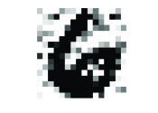
(b) Noisy

(c) es

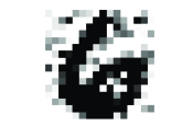
(d) Lasso

(e) Lasso-Gauss

Figure 6: Reconstruction of the digit “6” with $\sigma=0.5$.

(a) True

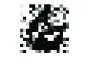
(b) Noisy

(c) es

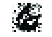
(d) Lasso

(e) Lasso-Gauss

Figure 7: Reconstruction of the digit “6” with $\sigma=1.0$.

For both $\sigma=0.5$ and $\sigma=1$, the experiment was repeated 250 times and the predictive performance of es was compared with that of the Lasso and Lasso-Gauss estimators. The results are represented in Figure 8 and Table 6.

\psfrag{a}[tr][.8][45]{{\sc es}}\psfrag{b}[tr][.8][45]{Lasso}\psfrag{c}[tr][.8][45]{Lasso-G}\includegraphics[width=227.62204pt]{box_6_sig05.eps}

\psfrag{a}[tr][.8][45]{{\sc es}}\psfrag{b}[tr][.8][45]{Lasso}\psfrag{c}[tr][.8][45]{Lasso-G}\includegraphics[width=227.62204pt]{box_6_sig10.eps}

Figure 8: Boxplots of the predictive performance $|\mu-\mathbf{X}\hat{\theta}|_{2}^{2}$ of the es, Lasso and Lasso-Gauss (Lasso-G) estimators computed from 250 replications of the model (7.4) with $\mu$ corresponding to the digit “6”. Left: $\sigma=0.5$. Right: $\sigma=1$. Notice that each graph uses a different scale.

	es	Lasso	Lasso-Gauss
$\sigma=0.5$	${\bf 26.57}$	59.49	40.55
	(4.57)	(5.28)	(14.58)
$\sigma=1.0$	${\bf 51.70}$	239.39	82.95
	(12.32)	(22.12)	(24.40)

Table 6: Means and standard deviations for $|\mu-\mathbf{X}\hat{\theta}|_{2}^{2}$ over 250 realizations of the es, Lasso and Lasso-Gauss estimators to reconstruct the digit “6”.

To conclude, we mention a byproduct of this simulation study. The coefficients of ${\tilde{\theta}^{\textsc{es}}}$ can be used to perform multi-class classification following the idea of Wright et al. (2009). The procedure consists in performing a majority vote on the features $x_{j}$ that are positively weighted by ${\tilde{\theta}^{\textsc{es}}}$, i.e., such that ${\tilde{\theta}^{\textsc{es}}}_{j}>0$. For the particular instance illustrated in Figure 6 (c), we see in Figure 9 that only a few features $x_{j}$ receive a large positive weight and that a majority of those correspond to the digit ”6”.

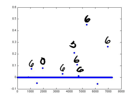
Figure 9: Coefficients of $\tilde{\tilde{\theta}}^{\textsc{es}}_{T}$, $T=10,000$ and the corresponding image.

8 Appendix

8.1 Lemmas for the upper bound

The following lemma is obtained by a variant of the “Maurey argument”, cf. also Barron (1993); Bunea et al. (2007b); Bickel et al. (2008) for similar but somewhat different results.

Lemma 8.1

For any $\theta^{*}\in{\rm I}\kern-1.79993pt{\rm R}^{M}\setminus\{0\}$, any integer $k\geq 1$, and any function $f$ we have

$$\min_{\theta:\begin{subarray}{l}|\theta|_{1}=|\theta^{*}|_{1}\\ M(\theta)\leq k\end{subarray}}\|f-{\sf f}_{\theta}\|^{2}\leq\|f-{\sf f}_{\theta^{*}}\|^{2}+\frac{|\theta^{*}|_{1}^{2}}{\min(k,M(\theta^{*}))}\,.$$

Proof. Fix $\theta^{*}\in{\rm I}\kern-1.79993pt{\rm R}^{M}\setminus\{0\}$ and an integer $k\geq 1$. Set $K=\min(k,M(\theta^{*}))$. Consider the multinomial parameter $p=(p_{1},\ldots,p_{M})^{\top}\in[0,1]^{M}$ with $p_{j}=|\theta^{*}_{j}|/|\theta^{*}|_{1},j=1,\ldots,M$, where $\theta^{*}_{j}$ are the components of $\theta^{*}$. Let $\kappa=(\kappa_{1},\ldots,\kappa_{M})^{\top}\in\{0,1,\ldots,M\}^{M}$ be the random vector with multinomial distribution $\mathcal{M}(K,p)$, i.e., let $\kappa_{j}=\sum_{s=1}^{K}{\rm 1}\kern-2.40005pt{\rm I}(I_{s}=j)$ where $I_{1},\ldots,I_{K}$ are i.i.d. random variables taking value $j\in\{1,\ldots,M\}$ with probability $p_{j}$, $j=1,\ldots,M$. In particular, we have $\mathcal{E}(\kappa_{j})=Kp_{j},j=1,\ldots,M$, where $\mathcal{E}$ denotes the expectation with respect to the multinomial distribution. As a result, for the random vector $\bar{\theta}\in{\rm I}\kern-1.79993pt{\rm R}^{M}$ with the components $\bar{\theta}_{j}=\kappa_{j}\mathop{\mathrm{sign}}(\theta^{*}_{j})|\theta^{*}|_{1}/K$ we have $\mathcal{E}(\bar{\theta}_{j})=\theta^{*}_{j}$ for $j=1,\ldots,M$ with the convention that $\mathop{\mathrm{sign}}(0)=0$. Moreover, using the fact that ${\rm Var}(\kappa_{j})=Kp_{j}(1-p_{j})$ and ${\rm Cov}(\kappa_{j},\kappa_{l})=-np_{j}p_{l}$ for $j\neq l$ (see, e.g., Bickel and Doksum, 2006, eq. (A.13.15), p. 462) we find that the covariance matrix of $\bar{\theta}$ is given by

$$\Sigma^{*}=\mathcal{E}\left[(\bar{\theta}-\theta^{*})(\bar{\theta}-\theta^{*})^{\top}\right]=\frac{|\theta^{*}|_{1}}{K}{\rm diag}(|\theta^{*}_{j}|)-\frac{1}{K}|\theta^{*}||\theta^{*}|^{\top}\,,$$

where $|\theta^{*}|=(|\theta^{*}_{j}|,\ldots,|\theta^{*}_{j}|)^{\top}$. Using a bias-variance decomposition together with the assumption $\max_{j}\|f_{j}\|\leq 1$, it yields that, for any function $f$,

$$\mathcal{E}\|f-{\sf f}_{\bar{\theta}}\|^{2}=\|f-{\sf f}_{\theta^{*}}\|^{2}+\frac{1}{n}\sum_{i=1}^{n}F(x_{i})^{\top}\Sigma^{*}F(x_{i})\leq\|f-{\sf f}_{\theta^{*}}\|^{2}+\frac{|\theta^{*}|_{1}^{2}}{K}\,,$$

where $F(x_{i})=(f_{1}(x_{i}),\ldots,f_{M}(x_{i}))^{\top}$, $i=1,\ldots,n$. Moreover, since $\bar{\theta}$ is such that $|\bar{\theta}|_{1}=|\theta^{*}|_{1}$ and $M(\bar{\theta})\leq K$, the lemma follows.    

Lemma 8.2

Fix $M,n\geq 1$ and assume that $\max_{j}\|f_{j}\|\leq 1$. For any function $\eta$ and any constant $\nu>0$ we have

$$\min_{\theta\in{\rm I}\kern-1.25995pt{\rm R}^{M}}\left\{\|{\sf f}_{\theta}-\eta\|^{2}+\nu^{2}\frac{M(\theta)}{n}\log\left(1+\frac{eM}{M(\theta)\vee 1}\right)\right\}\leq\min_{\theta\in{\rm I}\kern-1.25995pt{\rm R}^{M}}\left\{\|{\sf f}_{\theta}-\eta\|^{2}+{\tilde{c}}\bar{\varphi}_{n,M}(\theta)\right\}$$ (8.1)

where ${\tilde{c}}=\left(3+\frac{1}{e}\right)$, $\bar{\varphi}_{n,M}(0)=0$ and for $\theta\neq 0$,

$$\bar{\varphi}_{n,M}(\theta)=\left\{\begin{array}[]{ll}\min\left[\frac{\nu|\theta|_{1}}{\sqrt{n}}\sqrt{\log\left(1+\frac{eM\nu}{|\theta|_{1}\sqrt{n}}\right)},|\theta|_{1}^{2}\right],&{\rm if}\ \langle{\sf f}_{\theta},\eta\rangle\leq\|{\sf f}_{\theta}\|^{2},\\ \frac{\nu|\theta|_{1}}{\sqrt{n}}\sqrt{\log\left(1+\frac{eM\nu}{|\theta|_{1}\sqrt{n}}\right)}+\frac{\nu^{2}\log(1+eM)}{{\tilde{c}}n},&{\rm otherwise}\,.\end{array}\right.$$ (8.2)

Proof. Set

$$A=\min_{\theta\in{\rm I}\kern-1.25995pt{\rm R}^{M}}\left\{\|{\sf f}_{\theta}-\eta\|^{2}+\nu^{2}\frac{M(\theta)}{n}\log\left(1+\frac{eM}{M(\theta)\vee 1}\right)\right\}.$$

It suffices to consider ${\rm I}\kern-1.79993pt{\rm R}^{M}\setminus\{0\}$ instead of ${\rm I}\kern-1.79993pt{\rm R}^{M}$ since $A\leq\|{\sf f}_{0}-\eta\|^{2}+{\tilde{c}}\bar{\varphi}_{n,M}(0)=\|\eta\|^{2}$. Fix $\theta^{*}\in{\rm I}\kern-1.79993pt{\rm R}^{M}\setminus\{0\}$ and define

$$x^{*}=|\theta^{*}|_{1}\sqrt{n}/\ell,\quad\text{where}\ \ell=\nu\sqrt{\log\left(1+\frac{eM\nu}{|\theta^{*}|_{1}\sqrt{n}}\right)}\,.$$

Assume first $x^{*}\leq 1$. In this case we have

$$|\theta^{*}|_{1}^{2}\leq\nu\frac{|\theta^{*}|_{1}}{\sqrt{n}}\sqrt{\log\left(1+\frac{eM\nu}{|\theta^{*}|_{1}\sqrt{n}}\right)}\,.$$ (8.3)

The previous display yields that $\bar{\varphi}_{n,M}(\theta^{*})=|\theta^{*}|_{1}^{2}$. Moreover, if $\langle{\sf f}_{\theta^{*}},\eta\rangle\leq\|{\sf f}_{\theta^{*}}\|^{2}$, it holds

$$\|\eta\|^{2}\leq\|{\sf f}_{\theta^{*}}-\eta\|^{2}+\|{\sf f}_{\theta^{*}}\|^{2}\leq\|{\sf f}_{\theta^{*}}-\eta\|^{2}+|\theta^{*}|_{1}^{2}\,.$$

As a result,

$$A\leq\|\eta\|^{2}\leq\bar{\varphi}_{n,M}(\theta^{*})\quad\mbox{if}\ \langle{\sf f}_{\theta^{*}},\eta\rangle\leq\|{\sf f}_{\theta^{*}}\|^{2}\ \mbox{and}\ x^{*}\leq 1.$$ (8.4)

Set $k^{*}=\lceil x^{*}\rceil$, i.e., $k^{*}$ is the minimal integer greater than or equal to $x^{*}$. Using the monotonicity of the mapping $t\mapsto\frac{t}{n}\log\left(1+\frac{eM}{t}\right)$ for $t>0$, and Lemma 8.1 we get, for any $\theta^{*}\in{\rm I}\kern-1.79993pt{\rm R}^{M}\setminus\{0\}$ such that $k^{*}\leq M(\theta^{*})\,,$

$$A \leq \min_{\theta\in{\rm I}\kern-1.25995pt{\rm R}^{M}}\left\{\|{\sf f}_{\theta}-\eta\|^{2}+\nu^{2}\frac{M(\theta)}{n}\log\left(1+\frac{eM}{M(\theta)\vee 1}\right)\right\}$$

$$\leq \min_{1\leq k\leq M(\theta^{*})}\min_{\theta:M(\theta)\leq k}\left\{\|{\sf f}_{\theta}-\eta\|^{2}+\nu^{2}\frac{k}{n}\log\left(1+\frac{eM}{k}\right)\right\}$$

$$\leq \|{\sf f}_{\theta^{*}}-\eta\|^{2}+\min_{1\leq k\leq M(\theta^{*})}\left\{\nu^{2}\frac{k}{n}\log\left(1+\frac{eM}{k}\right)+\frac{|\theta^{*}|_{1}^{2}}{k}\right\}$$

$$\leq \|{\sf f}_{\theta^{*}}-\eta\|^{2}+\nu^{2}\frac{k^{*}}{n}\log\left(1+\frac{eM}{k^{*}}\right)+\frac{|\theta^{*}|_{1}^{2}}{k^{*}}\,.$$

On the other hand, if $\theta^{*}\in{\rm I}\kern-1.79993pt{\rm R}^{M}\setminus\{0\}$ and $k^{*}>M(\theta^{*})$, we use the simple bound

$$A \leq \|{\sf f}_{\theta^{*}}-\eta\|^{2}+\nu^{2}\frac{M(\theta^{*})}{n}\log\left(1+\frac{eM}{M(\theta^{*})\vee 1}\right)$$

$$\leq \|{\sf f}_{\theta^{*}}-\eta\|^{2}+\nu^{2}\frac{k^{*}}{n}\log\left(1+\frac{eM}{k^{*}}\right)\,.$$

In view of the last two displays, to conclude the proof it suffices to show that

$$\nu^{2}\frac{k^{*}}{n}\log\left(1+\frac{eM}{k^{*}}\right)+\frac{|\theta^{*}|_{1}^{2}}{k^{*}}\leq{\tilde{c}}\bar{\varphi}_{n,M}(\theta^{*})$$ (8.5)

for all $\theta^{*}\in{\rm I}\kern-1.79993pt{\rm R}^{M}\setminus\{0\}$. Note first that if $x^{*}\leq 1$, then $k^{*}=1$ and

$$\nu^{2}\frac{k^{*}}{n}\log\left(1+\frac{eM}{k^{*}}\right)+\frac{|\theta^{*}|_{1}^{2}}{k^{*}}\leq\frac{\nu^{2}\log(1+eM)}{n}+\nu\frac{|\theta^{*}|_{1}}{\sqrt{n}}\sqrt{\log\left(1+\frac{eM\nu}{|\theta^{*}|_{1}\sqrt{n}}\right)}\leq{\tilde{c}}\bar{\varphi}_{n,M}(\theta^{*})\,,$$

where we used (8.3) in the first inequality. Together with (8.4), this proves that $A\leq\|{\sf f}_{\theta^{*}}-\eta\|^{2}+{\tilde{c}}\bar{\varphi}_{n,M}(\theta^{*})$ for all $\theta^{*}\in{\rm I}\kern-1.79993pt{\rm R}^{M}\setminus\{0\}$ such that $x^{*}\leq 1$. Thus, to complete the proof of the lemma we only need to consider the case $x^{*}>1$. For $x^{*}>1$ we have

$$\bar{\varphi}_{n,M}(\theta^{*})\geq\nu\frac{|\theta^{*}|_{1}}{\sqrt{n}}\sqrt{\log\left(1+\frac{eM\nu}{|\theta^{*}|_{1}\sqrt{n}}\right)}\,.$$

As a result, we have

$$\frac{|\theta^{*}|_{1}^{2}}{k^{*}}\leq\frac{|\theta^{*}|_{1}\ell}{\sqrt{n}}\leq\bar{\varphi}_{n,M}(\theta^{*})\,.$$ (8.6)

Moreover, it holds $k^{*}\leq 2x^{*}=2|\theta^{*}|_{1}\sqrt{n}/\ell$ and since the function $t\mapsto\frac{t}{n}\log\left(1+\frac{eM}{t}\right)$ is increasing, we obtain

$$\frac{k^{*}}{n}\log\left(1+\frac{eM}{k^{*}}\right)\leq\frac{2|\theta^{*}|_{1}}{\ell\sqrt{n}}\log\left(1+\frac{eM\ell}{2|\theta^{*}|_{1}\sqrt{n}}\right)\,.$$

Thus, for $\ell\leq\nu$ we have

$$\frac{k^{*}}{n}\log\left(1+\frac{eM}{k^{*}}\right)\leq\frac{2|\theta^{*}|_{1}}{\ell\sqrt{n}}\log\left(1+\frac{eM\nu}{2|\theta^{*}|_{1}\sqrt{n}}\right)\leq\frac{2|\theta^{*}|_{1}\ell}{\nu^{2}\sqrt{n}}\leq\frac{2}{\nu^{2}}\bar{\varphi}_{n,M}(\theta^{*})\,.$$

For $\ell>\nu$ we use the inequality $\log(1+ab)\leq\log(1+a)+\log b,\forall\ a\geq 0,b\geq 1$, to obtain

$$\frac{k^{*}}{n}\log\left(1+\frac{eM}{k^{*}}\right) \leq \frac{2|\theta^{*}|_{1}}{\ell\sqrt{n}}\left[\log\left(1+\frac{eM\nu}{2|\theta^{*}|_{1}\sqrt{n}}\right)+\log\left(\frac{\ell}{\nu}\right)\right]$$

$$\leq \frac{2|\theta^{*}|_{1}}{\sqrt{n}}\left(\frac{\ell}{\nu^{2}}+\frac{\log(\ell/\nu)}{\ell}\right)\leq\left(2+\frac{1}{e}\right)\frac{|\theta^{*}|_{1}\ell}{\nu^{2}\sqrt{n}}$$

$$\leq \left(2+\frac{1}{e}\right)\frac{1}{\nu^{2}}\bar{\varphi}_{n,M}(\theta^{*})\,.$$

Thus, in both cases $\frac{k^{*}}{n}\log\left(1+\frac{eM}{k^{*}}\right)\leq(2+1/e)\nu^{-2}\bar{\varphi}_{n,M}(\theta^{*})$. Combining this with (8.6) we get (8.5).    

8.2 Proof of Theorem 5.2

Applying the randomization scheme described in Nemirovski (2000), p.211, we create from the sample $y_{1},\dots,y_{n}$ satisfying (5.2) two independent subsamples with “equivalent” sizes $\lceil n(1-1/\log\log n)\rceil$ and $n-\lceil n(1-1/\log\log n)\rceil$. We use the first subsample to construct the es estimator and the soft thresholding estimator $\hat{\theta}^{\textsc{soft}}$, the latter attaining asymptotically the rate $\psi_{n}^{01}(\theta)$ for all $\theta\in{\rm I}\kern-1.79993pt{\rm R}^{n}$. We then use the second subsample to aggregate them, for example, as described in Nemirovski (2000). Then the aggregated estimator denoted by $\tilde{\theta}^{*}$ satisfies, for all $\theta\in{\rm I}\kern-1.79993pt{\rm R}^{n}$,

$$E_{\theta}|\tilde{\theta}^{*}-\theta|_{2}^{2} \leq \min\left\{E_{\theta}|\hat{\theta}^{\textsc{soft}}-\theta|_{2}^{2},\,E_{\theta}|\tilde{\theta}^{\textsc{es}}-\theta|_{2}^{2}\right\}+\frac{C\log\log n}{n}$$

$$\leq \min(\psi_{n}^{01}(\theta),\psi_{n}^{*}(\theta))(1+o(1))+\frac{C\log\log n}{n}$$

where $C>0$ is an absolute constant and $o(1)\to 0$ as $n\to\infty$ uniformly in $\theta\in{\rm I}\kern-1.79993pt{\rm R}^{n}$. Set

$$\tilde{\psi}_{n}(\theta)=\min(\psi_{n}^{01}(\theta),\psi_{n}^{*}(\theta))+\frac{C\log\log n}{n}.$$

Then (5.10) follows immediately. Next, $\psi_{n}^{01}(\theta)\geq 2(\log n)/n$, so that for all $\theta\in{\rm I}\kern-1.79993pt{\rm R}^{n}$,

$$\frac{\psi_{n}^{01}(\theta)}{\tilde{\psi}_{n}(\theta)}\geq\frac{\psi_{n}^{01}(\theta)}{\psi_{n}^{01}(\theta)+C(\log\log n)/n}\geq\frac{2(\log n)/n}{2(\log n)/n+C(\log\log n)/n}\,,$$

which implies (5.11). Finally, to prove (5.12) it is enough to notice that since $\psi_{n}^{01}(\theta)\geq 2(\log n)/n$,

$$\frac{\tilde{\psi}_{n}(\theta)}{\psi_{n}^{01}(\theta)}\leq\frac{\psi_{n}^{*}(\theta)+C(\log\log n)/n}{\psi_{n}^{01}(\theta)}\leq\frac{\psi_{n}^{*}(\theta)}{\psi_{n}^{01}(\theta)}+\frac{C\log\log n}{2\log n}$$

and to use (5.8).

8.3 Proof of Theorem 5.3

Clearly (5.17) follows from (5.18) since in the latter $\eta$ is fixed and equal to one particular function $\eta={\sf f}_{\theta}$.

We now prove (5.18). Let $\mathcal{H}=\{f_{1},\ldots,f_{M}\}$ be any dictionary in $\mathcal{D}(S\wedge\bar{m},{\kappa})$ with the corresponding $\underline{\kappa}$ and $\bar{\kappa}$ such that $\underline{\kappa}/\bar{\kappa}=\kappa$. For any $k\in\{1,\ldots,M\}$, let $\Omega_{k}$ be the subset of $\mathcal{P}=\{0,1\}^{M}$ defined by

$$\Omega_{k}:=\left\{{\sf p}\in\mathcal{P}\,:\,|{\sf p}|=k\right\}.$$ (8.7)

We consider the class of functions

$$\mathcal{F}_{k}(\delta):=\left\{f=\frac{\delta}{k}\tau{\sf f}_{\sf p}\ :\ {\sf p}\in\Omega_{k}\right\}\,,$$

where $0<\tau\leq 1$ will be chosen later. Note that functions in $\mathcal{F}_{k}(\delta)$ are of the form ${\sf f}_{\theta}$ with $\theta\in{\rm I}\kern-1.79993pt{\rm R}^{M}_{+}\setminus\{0\}$, $M(\theta)=k$ and $|\theta|_{1}=\tau\delta\leq\delta$. Thus, to prove (5.18), it is sufficient to show that, for any estimator $T_{n}$,

$$\sup_{\eta\in\mathcal{G}}E_{\eta}\|{T}_{n}-\eta\|^{2}>c_{*}\kappa\zeta_{n,M,\mathrm{rk}(\mathbf{X})}(S,\delta)\,,$$ (8.8)

for some subset $\mathcal{G}\subset\mathcal{F}_{\bar{S}}(\delta)$ where $\bar{S}=[S\wedge\bar{m}\wedge(M/2)]$ and $[\cdot]$ denotes the integer part. Note that $\bar{S}\geq 1$ since $M\geq 2$ and $S\wedge\bar{m}\geq 1$.

In what follows we will use the fact that for $f,g\in\mathcal{F}_{\bar{S}}(\delta)$ the difference $f-g$ is of the form ${\sf f}_{\theta}$ with some $\theta\in\mathcal{P}_{2\bar{S}}$, so that in view of (5.14), $\|f-g\|^{2}$ is bracketed by the multiples of $|\theta|^{2}_{2}$ with this value of $\theta$.

We now consider three cases, depending on the value of the integer $m$ defined in (5.16).

Case $(1)$: $m=0$. Use Lemma 8.3 to construct a subset $\mathcal{G}_{(1)}\subseteq\mathcal{F}_{1}(\delta)\subseteq\mathcal{F}_{\bar{S}}(\delta)$ with cardinality $s_{(1)}\geq(1+eM)^{C_{1}}$ and such that

$$\|f-g\|^{2}\geq\frac{\tau^{2}\delta^{2}\underline{\kappa}}{2}\,,\quad\forall\ f,g\in\mathcal{G}_{(1)},f\neq g\,.$$ (8.9)

Since $m=0$, inequality (5.16) is violated for $m=1$, so that

$$\delta^{2}<\frac{\sigma^{2}}{n}\log\left(1+eM\right)\leq\frac{\sigma^{2}}{nC_{1}}\log(s_{(1)})\,.$$ (8.10)

Case $(2)$: $m\geq 1,S\wedge(M/2)\geq m$. Then $\bar{m}=m=\bar{S}$ and $m\leq M/2$, so that we have $\min(m,M-m)=m$, and Lemma 8.3 guarantees that there exists $\mathcal{G}_{(2)}\subseteq\mathcal{F}_{m}(\delta)=\mathcal{F}_{\bar{S}}(\delta)$ with cardinality $s_{(2)}\geq(1+eM/m)^{C_{1}m}$ and such that

$$\|f-g\|^{2}\geq\frac{\tau^{2}\delta^{2}\underline{\kappa}}{4m}\,,\quad\forall\ f,g\in\mathcal{G}_{(2)},f\neq g\,.$$

To bound from below the quantity $\delta^{2}/m$, observe that from the definition of $m$ we have

$$\frac{\delta^{2}}{m}\geq\frac{\delta\sigma}{\sqrt{n}}\sqrt{\log\left(1+\frac{eM}{m}\right)}\geq\frac{\delta\sigma}{\sqrt{n}}\sqrt{\log\left(1+\frac{eM\sigma}{\delta\sqrt{n}}\right)}\,.$$ (8.11)

The previous two displays yield

$$\|f-g\|^{2}\geq\frac{\tau^{2}\underline{\kappa}\delta\sigma}{4\sqrt{n}}\sqrt{\log\left(1+\frac{eM\sigma}{\delta\sqrt{n}}\right)}\,.$$ (8.12)

Note that in this case

$$m+1>\frac{\delta\sqrt{n}}{\sigma\sqrt{\log\left(1+\frac{eM}{m+1}\right)}}\,,$$

so that

$$\frac{\delta^{2}}{m}\leq\frac{2\delta^{2}}{m+1}<2(m+1)\frac{\sigma^{2}}{n}\log\left(1+\frac{eM}{m+1}\right)\leq 4m\frac{\sigma^{2}}{n}\log\left(1+\frac{eM}{m}\right)\leq\frac{4\sigma^{2}}{nC_{1}}\log(s_{(2)})\,.$$ (8.13)

Case $(3)$: $m\geq 1,S\wedge(M/2)<m$. Then $\bar{S}=[S\wedge(M/2)]<m$. Moreover, we have $\min(\bar{S},M-\bar{S})=\bar{S}$ and using Lemma 8.3, for any positive $\bar{\delta}\leq\delta$ we can construct $\mathcal{G}_{(3)}\subseteq\mathcal{F}_{\bar{S}}(\bar{\delta})$ with cardinality $s_{(3)}\geq\big{(}1+eM/\bar{S}\big{)}^{C_{1}\bar{S}}$ and such that

$$\|f-g\|^{2}\geq\frac{\tau^{2}\bar{\delta}^{2}\underline{\kappa}}{4\bar{S}}\,,\quad\forall\ f,g\in\mathcal{G}_{(3)},f\neq g\,,$$

Take

$$\bar{\delta}:=\sigma\frac{\bar{S}}{\sqrt{n}}\sqrt{\log\left(1+\frac{eM}{\bar{S}}\right)}\leq\sigma\frac{m}{\sqrt{n}}\sqrt{\log\left(1+\frac{eM}{m}\right)}\leq\delta\,,$$

where, in the last inequality, we used the definition of $m$. Next, note that $\bar{S}=[S\wedge(M/2)]1\geq S/4$ since $M\geq 2$. Then

$$\|f-g\|^{2}\geq\frac{\tau^{2}\underline{\kappa}\sigma^{2}\bar{S}}{4n}\log\left(1+\frac{eM}{\bar{S}}\right)\geq\frac{\tau^{2}\underline{\kappa}\sigma^{2}S}{16n}\log\left(1+\frac{4eM}{S}\right)\,.$$ (8.14)

In addition, we have

$$\frac{\bar{\delta}^{2}}{\bar{S}}=\bar{S}\frac{\sigma^{2}}{n}\log\left(1+\frac{eM}{\bar{S}}\right)\leq\frac{\sigma^{2}}{nC_{1}}\log(s_{(3)})\,.$$ (8.15)

Since the random variables $\xi_{i},i=1,\ldots,n$ are i.i.d. Gaussian $\mathcal{N}(0,\sigma^{2})$, for any $f,g\in\mathcal{G}_{(j)}$, $j\in\{1,2,3\}$, the Kullback-Leibler divergence $\mathcal{K}(P_{f},P_{g})$ between $P_{f}$ and $P_{g}$ is given by

$$\mathcal{K}(P_{f},P_{g})=\frac{n}{2\sigma^{2}}\|f-g\|^{2}\leq\frac{n\tau^{2}\delta_{(j)}^{2}\bar{\kappa}}{\sigma^{2}k_{(j)}}\,,$$

where $\delta_{(1)}=\delta_{(2)}=\delta,\delta_{(3)}=\bar{\delta},k_{(1)}=1,k_{(2)}=m,k_{(3)}=\bar{S}$. Using respectively (8.10) in case $(1)$, (8.13) in case $(2)$ and (8.15) in case $(3)$, and choosing $\tau^{2}=\min(C_{1}/(32\bar{\kappa}),1)$ (note that we need $\tau\leq 1$ by construction) we obtain

$$\mathcal{K}(P_{f},P_{g})\leq\frac{4\tau^{2}\bar{\kappa}}{C_{1}}\log s_{(j)}\leq\frac{\log s_{(j)}}{8}\,,\quad\forall\ f,g\in\mathcal{G}_{(j)},\ j=1,2,3.$$ (8.16)

Combining (8.9), (8.12) and (8.14) together with (8.16), we find that the conditions of Theorem 2.7 in Tsybakov (2009) are satisfied and use it to obtain (8.8).    

8.4 A lemma for minimax lower bound

Here we give a result related to subset extraction, which is a generalization of the Varshamov-Gilbert lemma used to prove minimax lower bounds (see, e.g., a recent survey in Tsybakov (2009)[Chap. 2]). For any $M\geq 1$, $k\in\{1,\ldots,M-1\}$, let $\Omega_{k}^{M}$ be the subset of $\{0,1\}^{M}$ defined by:

$$\Omega_{k}^{M}:=\left\{\omega\in\{0,1\}^{M}\,:\,\sum_{j=1}^{M}\omega_{j}=k\right\}$$

The next lemma is a modification of Birgé and Massart (2001, Lemma 4). The difference is that we cover any $M\geq 2$, $1\leq k\leq M$. The result of Birgé and Massart (2001) is proved for even integer $k$ such that $M\geq 3k\geq 6$. The price we pay for considering general $M,k$ is only in terms of constants, which is sufficient for our purposes.

Lemma 8.3

Let $M\geq 2$ and $1\leq k\leq M$ be two integers and define $\bar{k}=\min(k,M-k)$. Then there exists a subset $\Omega$ of $\Omega_{k}^{M}$ such that the Hamming distance $\rho(\omega,\omega^{\prime})=\sum_{j=1}^{M}{\rm 1}\kern-2.40005pt{\rm I}(\omega_{j}\neq\omega_{j}^{\prime})$ satisfies

$$\rho(\omega,\omega^{\prime})\geq\frac{\bar{k}+1}{4},\qquad\forall\,\omega,\omega^{\prime}\in\Omega:\ \omega\neq\omega^{\prime}\,,$$

and $s=\mathop{\mathrm{card}}(\Omega)$ satisfies

$$\log(s)\geq C_{1}\bar{k}\log\left(1+\frac{eM}{\bar{k}}\right)\,,$$

for some numerical constant $C_{1}\geq 9\cdot 10^{-4}$.

Proof. (i) Consider first the case where $k=2p$ for some integer $p\geq 1$ and $M\geq 6p$. Lemma 4 in Birgé and Massart (2001) ensures the existence of a subset $\Omega^{(1)}$ of $\Omega_{k}^{M}$ such that $\rho(\omega,\omega^{\prime})\geq k/2+1\geq(k+1)/2$ for any $\omega\neq\omega^{\prime}\in\Omega^{(1)}$ and

$$\log\left(\mathop{\mathrm{card}}(\Omega^{(1)})\right)\geq p\left[\log(M/p)-\log(16)+1\right]=\frac{k}{2}\log\left(\frac{eM}{8k}\right)\,.$$ (8.17)

(ii) Next, if $k=2p+1$ for some integer $p\geq 18$ and $M\geq 6p+3$, let $\widetilde{\Omega}\subset\Omega^{M-1}_{k-1}$ be the set obtained by Lemma 4 in Birgé and Massart (2001). We have $\rho(\omega,\omega^{\prime})\geq(k+1)/2$ for any $\omega,\omega^{\prime}\in\widetilde{\Omega},\omega^{\prime}\neq\omega$ and

$$\log\left(\mathop{\mathrm{card}}(\widetilde{\Omega})\right)\geq\frac{k-1}{2}\log\left(\frac{e(M-1)}{8(k-1)}\right)\geq\frac{k}{3}\log\left(\frac{eM}{8k}\right)\,,$$ (8.18)

where we used the fact that $3\leq k\leq M$. Define now the set

$$\Omega^{(2)}=\left\{\omega\in\{0,1\}^{M}\,:\,\omega=(1,\tilde{\omega})\,,\ \tilde{\omega}\in\widetilde{\Omega}\right\}\,.$$

We have $\Omega^{(2)}\subset\Omega^{M}_{k}$, $\mathop{\mathrm{card}}(\Omega^{(2)})=\mathop{\mathrm{card}}(\widetilde{\Omega})$ and $\rho(\omega,\omega^{\prime})\geq(k+1)/2$ for any $\omega,\omega^{\prime}\in\Omega^{(2)},\omega^{\prime}\neq\omega$.

So far, we have fully covered $M,k$ such that $M\geq 3k$, $k\geq 36$. We consider now respectively the cases (iii) $2k\leq M<3k,k\geq 72$, (iv) $k\leq 71,M\geq 2k$, and (v) $M<2k$.

(iii) If $2k\leq M<3k$, $k\geq 72$, let $k^{\prime}$ be the integer part of $k/2$: $k^{\prime}=[k/2]\geq 36$, and observe that $3k^{\prime}\leq M^{\prime}$ where $M^{\prime}=M-(k-k^{\prime})\leq M$. Therefore, we can apply the preceding results to ensure that there exists a subset $\bar{\Omega}$ of $\Omega_{k^{\prime}}^{M^{\prime}}$ such that

$$\log\left(\mathop{\mathrm{card}}(\bar{\Omega})\right)\geq\frac{k^{\prime}}{3}\log\left(\frac{eM^{\prime}}{8k^{\prime}}\right)\,$$

and $\rho(\omega,\omega^{\prime})\geq(k^{\prime}+1)/2$ for any $\omega,\omega^{\prime}\in\bar{\Omega}$, $\omega\neq\omega^{\prime}$. Since $k^{\prime}\geq k/3$, we obtain

$$\log\left(\mathop{\mathrm{card}}(\bar{\Omega})\right)\geq\frac{k}{9}\log\left(\frac{eM^{\prime}}{8k^{\prime}}\right)\,.$$ (8.19)

To embed $\bar{\Omega}$ in $\Omega_{k}^{M}$, define

$$\Omega^{(3)}=\left\{\omega\in\{0,1\}^{M}\,:\,\omega=(\underbrace{1,\dots,1}_{k-k^{\prime}\ \text{times}},\bar{\omega})\,,\ \bar{\omega}\in\bar{\Omega}\right\}\,.$$

We have $\Omega^{(3)}\subset\Omega^{M}_{k}$, $\mathop{\mathrm{card}}(\Omega^{(3)})=\mathop{\mathrm{card}}(\bar{\Omega})$ and $\rho(\omega,\omega^{\prime})\geq(k^{\prime}+1)/2\geq(k+1)/4$ for any $\omega,\omega^{\prime}\in\Omega^{(3)},\omega^{\prime}\neq\omega$.

(iv) If $k\leq 71,M\geq 2k$, consider the set $\Omega^{(4)}=\{\omega^{(1)},\ldots,\omega^{([M/k])}\}\subset\Omega_{k}^{M}$, such that, for any $j=1,\ldots,[M/k]$, the $l$-th coordinate of $\omega^{(j)}$ satisfies $\omega^{(j)}_{l}=1$ if and only if $(j-1)k+1\leq l\leq jk$. We have $\rho(\omega,\omega^{\prime})=2k\geq(k+1)/4$ for any $\omega,\omega^{\prime}\in\Omega^{(4)},\omega^{\prime}\neq\omega$ and

$$\log\left(\mathop{\mathrm{card}}(\Omega^{(4)})\right)=\log\left(\left[\frac{M}{k}\right]\right) \geq \frac{\log 2}{\log(1+2e)}\log\left(1+\frac{eM}{k}\right)$$ (8.20)

$$\geq \frac{k}{71}\frac{\log 2}{\log(1+2e)}\log\left(1+\frac{eM}{k}\right)$$

$$\geq 0.005k\log\left(1+\frac{eM}{k}\right).$$

Note that (i)–(iv) cover all $M\geq 2k$ and $k\geq 1$, and in these cases $\bar{k}=k$. We now use (8.17), (8.18) and (8.19) jointly with the following inequality

$$\frac{1}{9}\log\left(\frac{x}{8}\right)\geq\frac{\log\left(\frac{3e}{8}\right)}{9\log(1+3e)}\log(1+x)\geq 0.0009\log(1+x)\,,\quad x\geq 3e\,.$$

This yields the result of the lemma for cases (i), (ii) and (iii) since in these cases $M/k\geq 3$ and $M^{\prime}/k^{\prime}\geq 3$. For case (iv) we use directly (8.20). Thus, the lemma is proved for $M\geq 2k$.

(v) Finally, if $M<2k$, or equivalently, when $M-k<k$, we can reproduce all the arguments above with $k$ replaced by $\bar{k}=M-k$ which satisfies $2\bar{k}\leq M$. In each case, $i=1,\dots,4$, we obtain the subsets $\bar{\Omega}^{(i)}\subset\Omega_{\bar{k}}^{M}$ analogous to $\Omega^{(i)}$ in (i)–(iv). They are uniquely mapped into $\Omega_{k}^{M}$ by applying the bijection $\omega\mapsto{\bf 1}-\omega$, where ${\bf 1}=(1\,\ldots,1)\in\{0,1\}^{M}$.    

Acknowledgement. We would like to thank Victor Chernozhukov for a helpful discussion of the paper.

References

• Abramovich et al. (2006) Abramovich, F., Benjamini, Y., Donoho, D. L. and Johnstone, I. M. (2006). Adapting to unknown sparsity by controlling the false discovery rate. Ann. Statist., 34 584–653.
• Alquier and Lounici (2010) Alquier, P. and Lounici, K. (2010). PAC-Bayesian bounds for sparse regression estimation with exponential weights. URL http://hal.archives-ouvertes.fr/hal-00465801.
• Baraniuk et al. (2008) Baraniuk, R., Davenport, M., DeVore, R. and Wakin, M. (2008). A simple proof of the restricted isometry property for random matrices. Constr. Approx., 28 253–263.
• Barron (1993) Barron, A. R. (1993). Universal approximation bounds for superpositions of a sigmoidal function. IEEE Trans. Inform. Theory, 39 930–945.
• Bickel et al. (2008) Bickel, P., Ritov, Y. and Tsybakov, A. (2008). Hierarchical selection of variables in sparse high-dimensional regression. ArXiv:0801.1158.
• Bickel and Doksum (2006) Bickel, P. J. and Doksum, K. A. (2006). Mathematical statistics: basic ideas and selected topics, vol. 1. 2nd ed. Updated printing. Prentice-Hall.
• Bickel et al. (2009) Bickel, P. J., Ritov, Y. and Tsybakov, A. B. (2009). Simultaneous analysis of lasso and Dantzig selector. Ann. Statist., 37 1705–1732.
• Birgé and Massart (2001) Birgé, L. and Massart, P. (2001). Gaussian model selection. J. Eur. Math. Soc. (JEMS), 3 203–268.
• Bühlmann and van de Geer (2009) Bühlmann, P. and van de Geer, S. (2009). On the conditions used to prove oracle results for the lasso. Electron. J. Stat., 3 1360–1392.
• Bunea et al. (2007a) Bunea, F., Tsybakov, A. and Wegkamp, M. (2007a). Sparsity oracle inequalities for the Lasso. Electron. J. Stat., 1 169–194 (electronic).
• Bunea et al. (2007b) Bunea, F., Tsybakov, A. B. and Wegkamp, M. H. (2007b). Aggregation for Gaussian regression. Ann. Statist., 35 1674–1697.
• Candes (2008) Candes, E. (2008). The restricted isometry property and its implications for compressed sensing. Comptes rendus-Mathématique, 346 589–592.
• Candes and Tao (2007) Candes, E. and Tao, T. (2007). The Dantzig selector: statistical estimation when $p$ is much larger than $n$. Ann. Statist., 35 2313–2351.
• Dalalyan and Tsybakov (2008) Dalalyan, A. and Tsybakov, A. (2008). Aggregation by exponential weighting, sharp pac-bayesian bounds and sparsity. Machine Learning, 72 39–61.
• Dalalyan and Tsybakov (2010) Dalalyan, A. and Tsybakov, A. B. (2010). Mirror averaging with sparsity priors. ArXiv.org:1003.1189.
• Dalalyan and Tsybakov (2007) Dalalyan, A. S. and Tsybakov, A. B. (2007). Aggregation by exponential weighting and sharp oracle inequalities. In Learning theory, vol. 4539 of Lecture Notes in Comput. Sci. Springer, Berlin, 97–111.
• Dalalyan and Tsybakov (2009) Dalalyan, A. S. and Tsybakov, A. B. (2009). Sparse regression learning by aggregation and langevin montecarlo. ArXiv:0903.1223.
• Donoho and Johnstone (1994a) Donoho, D. L. and Johnstone, I. M. (1994a). Ideal spatial adaptation by wavelet shrinkage. Biometrika, 81 425–455.
• Donoho and Johnstone (1994b) Donoho, D. L. and Johnstone, I. M. (1994b). Minimax risk over $l_{p}$-balls for $l_{q}$-error. Probab. Theory Related Fields, 99 277–303.
• Donoho et al. (1992) Donoho, D. L., Johnstone, I. M., Hoch, J. C. and Stern, A. S. (1992). Maximum entropy and the nearly black object. J. Roy. Statist. Soc. Ser. B, 54 41–81. With discussion and a reply by the authors.
• Fan and Li (2001) Fan, J. and Li, R. (2001). Variable selection via nonconcave penalized likelihood and its oracle properties. J. Amer. Statist. Assoc., 96 1348–1360.
• Foster and George (1994) Foster, D. P. and George, E. I. (1994). The risk inflation criterion for multiple regression. Ann. Statist., 22 1947–1975.
• George (1986a) George, E. I. (1986a). Combining minimax shrinkage estimators. J. Amer. Statist. Assoc., 81 437–445.
• George (1986b) George, E. I. (1986b). Minimax multiple shrinkage estimation. Ann. Statist., 14 188–205.
• Giraud (2008) Giraud, C. (2008). Mixing least-squares estimators when the variance is unknown. Bernoulli, 14 1089–1107.
• Hastie et al. (2001) Hastie, T., Tibshirani, R. and Friedman, J. (2001). The elements of statistical learning. Springer Series in Statistics, Springer-Verlag, New York. Data mining, inference, and prediction, URL http://www-stat.stanford.edu/~tibs/ElemStatLearn/.
• Koh et al. (2008) Koh, K., Kim, S.-J. and Boyd, S. (2008). l1_ls: A Matlab solver for l1-regularized least squares problems. BETA version, May 10 2008, URL http://www.stanford.edu/~boyd/l1_ls.
• Koltchinskii (2008) Koltchinskii, V. (2008). Oracle inequalities in empirical risk minimization and sparse recovery problems. To appear in St Flour lecture notes.
• Koltchinskii (2009a) Koltchinskii, V. (2009a). The Dantzig selector and sparsity oracle inequalities. Bernoulli, 15 799–828.
• Koltchinskii (2009b) Koltchinskii, V. (2009b). Sparsity in penalized empirical risk minimization. Ann. Inst. Henri Poincaré Probab. Stat., 45 7–57.
• LeCun et al. (1990) LeCun, Boser, B., Denker, J. S., Henderson, D., Howard, R. E., Hubbard, W. and Jackel, L. D. (1990). Handwritten digit recognition with a back-propagation network. In Advances in Neural Information Processing Systems. Morgan Kaufmann, 396–404.
• Leung and Barron (2006) Leung, G. and Barron, A. R. (2006). Information theory and mixing least-squares regressions. IEEE Trans. Inform. Theory, 52 3396–3410.
• Lounici (2007) Lounici, K. (2007). Generalized mirror averaging and $D$-convex aggregation. Math. Methods Statist., 16 246–259.
• Nemirovski (2000) Nemirovski, A. (2000). Topics in non-parametric statistics. In Lectures on probability theory and statistics (Saint-Flour, 1998), vol. 1738 of Lecture Notes in Math. Springer, Berlin, 85–277.
• Raskutti et al. (2009) Raskutti, G., Wainwright, M. J. and Yu, B. (2009). Minimax rates of estimation for high-dimensional linear regression over $\ell_{q}$-balls. ArXiv:0910.2042.
• Rigollet (2009) Rigollet, P. (2009). Maximum likelihood aggregation and misspecified generalized linear models. ArXiv:0911.2919.
• Robert and Casella (2004) Robert, C. and Casella, G. (2004). Monte Carlo statistical methods. Springer Verlag.
• Tsybakov (2003) Tsybakov, A. B. (2003). Optimal rates of aggregation. In COLT (B. Schölkopf and M. K. Warmuth, eds.), vol. 2777 of Lecture Notes in Computer Science. Springer, 303–313.
• Tsybakov (2009) Tsybakov, A. B. (2009). Introduction to nonparametric estimation. Springer Series in Statistics. New York, NY: Springer. xii.
• van de Geer (2008) van de Geer, S. A. (2008). High-dimensional generalized linear models and the lasso. Ann. Statist., 36 614–645.
• Wright et al. (2009) Wright, J., Yang, A. Y., Ganesh, A., Sastry, S. S. and Ma, Y. (2009). Robust face recognition via sparse representation. IEEE Trans. Pattern Anal. Mach. Intell., 31 210–227.
• Zhang (2010) Zhang, C.-H. (2010). Nearly unbiased variable selection under minimax concave penalty. Ann. Statist., 38 894–942.
• Zhang and Huang (2008) Zhang, C.-H. and Huang, J. (2008). The sparsity and bias of the LASSO selection in high-dimensional linear regression. Ann. Statist., 36 1567–1594.
• Zhang and Melnik (2009) Zhang, C.-H. and Melnik, O. (2009). plus: Penalized Linear Unbiased Selection. R package version 0.8, URL http://CRAN.R-project.org/package=plus.
• Zhang (2009) Zhang, T. (2009). Some sharp performance bounds for least squares regression with $L_{1}$ regularization. Ann. Statist., 37 2109–2144.