Accounting for Stochastic Fluctuations when Analysing Integrated Light of Star Clusters. I: First Systematics

Abstract

Context. Star clusters are studied widely both as benchmarks for stellar evolution models and in their own right. Cluster age distributions and mass distributions within galaxies are probes of star formation histories, and of cluster formation and disruption processes. The vast majority of clusters in the Universe is small, and it is well known that the integrated fluxes and colours of all but the most massive ones have broad probability distributions, due to small numbers of bright stars.

Aims. This paper goes beyond the description of predicted probability distributions, and presents results of the analysis of cluster energy distributions in an explicitly stochastic context.

Methods. The method developed is Bayesian. It provides posterior probability distributions in the age-mass-extinction space, using multi-wavelength photometric observations and a large collection of Monte-Carlo simulations of clusters of finite stellar masses. The main priors are the assumed intrinsic distributions of current mass and current age for clusters in a galaxy. Both UBVI and UBVIK data sets are considered, and the study conducted in this paper is restricted to the solar metallicity.

Results. We first use the collection of simulations to reassess and explain errors arising from the use of standard analysis methods, which are based on continuous population synthesis models: systematic errors on ages and random errors on masses are large, while systematic errors on masses tend to be smaller. The age-mass distributions obtained after analysis of a synthetic sample are very similar to those found for real galaxies in the literature. The Bayesian approach on the other hand, is very successful in recovering the input ages and masses over ages ranging between 20 Myr and 1.5 Gyr, with only limited systematics that we explain.

Conclusions. Taking stochasticity into account is important, more important for instance than the choice of adding or removing near-IR data in many cases. We found no immediately obvious reason to reject priors inspired by previous (standard) analyses of cluster populations in galaxies, i.e. cluster distributions that scale with mass as $M^{-2}$ and are uniform on a logarithmic age scale.

1 Introduction

In the early decades of astrophysics, star clusters have been our main key to the understanding of stellar evolution. While clusters continue to provide precious constraints on stellar physics, they are today studied in their own right and as tracers of the histories of galaxies. It has become clear that a significant fraction of star formation occurs in clusters, and that events such as interacting galaxies can trigger their formation (Harris, 1991; Meurer et al., 1995; Barton, Geller, & Kenyon, 2000; Di Matteo et al., 2007). Questions have been raised regarding the IMF in clusters in various environments, about the systematic trends in their colour distributions, about their lifetimes as gravitationally bound objects and about the initial and current cluster mass functions.

Resolved observations of individual stars remain the most precise way of investigating the nature of clusters and will be possible out to distances of 10 Mpc with future extremely large telescopes. However measurements of the integrated light of unresolved star clusters reach far beyond this scale already today, and will remain the path of choice for the studies of large samples.

All our studies of individual clusters and of cluster populations in galaxies rest on our ability to estimate their current ages, masses and metallicities, while accounting for extinction. The standard method of analysis of integrated cluster light is based on the direct comparison of the observed colours with predictions from continuous population synthesis models. These models predict fluxes with the assumption that each mass bin along the stellar mass function (SMF) is populated according to the average value given by this SMF. Studies based on continuous population synthesis models have led to results that have a large impact on today’s description of cluster “demographics”. For instance, it is now usually admitted that the current cluster mass function decreases with mass as a power law with an index close to $-2$ (Zhang & Fall, 1999; Bik et al., 2003; Boutloukos & Lamers, 2003) and the debate on the cluster survival rate also rests on distributions obtained using continuous models (Vesperini, 1998; Fall & Zhang, 2001; Lada & Lada, 2003; Rafelski & Zaritsky, 2005). The continuous approach has been coupled with statistical data analysis, for instance to provide the impression that including near-IR photometry (K band) solves the age-metallicity degeneracy for clusters (Goudfrooij et al., 2001; Puzia et al., 2002; Anders et al., 2004; Bridžius et al., 2008). Still in the context of continuous population synthesis, Cid Fernandes & González Delgado (2010) followed by González Delgado & Cid Fernandes (2010) developed a Bayesian analysis of the integrated spectra of star clusters.

The continuous population synthesis models are strictly valid only in the limit of a stellar population containing an infinite number of stars. Real clusters, however, count a finite number of stars. Furthermore most of the light is provided by a very small number of bright stars, in particular in the near-IR. The so-called stochastic fluctuations in the integrated photometric properties are the result of the random presence of these luminous stars. Some of these can be quantified using selected information provided by continuous population synthesis models (e.g. Lançon & Mouhcine, 2000; Cerviño et al., 2002; Cerviño & Luridiana, 2004, 2006), but others require the use of discrete population synthesis models (Barbaro & Bertelli, 1977; Girardi & Bica, 1993; Bruzual, 2002; Deveikis et al., 2008; Popescu & Hanson, 2009; Piskunov et al., 2009). The predicted luminosity and colour distributions depend strongly on the total mass (or star number) in the cluster, and can be far from Gaussian even when the total mass exceeds $10^{5}$ M_⊙. The most probable colours are offset from those predicted by continuous population synthesis when masses are below $10^{4}$ M_⊙, because the single most luminous star in such clusters will be more often on the main sequence than in the red giant phases of evolution. Attempts to describe the colour distributions analytically have made progress (e.g. Cerviño & Luridiana, 2006), but are not yet easily applicable.

The present piece of work is based on discrete population synthesis. For the first time, we use the discrete models not only to predict colour distributions but to analyse the energy distributions of clusters. We present a Bayesian approach to the probabilistic determination of age, mass and extinction, based on a large library of Monte-Carlo simulations of clusters. This method is a close analog to the one introduced by Kauffmann et al. (2003) for the study of star formation histories in the Sloan Digital Sky Survey. However the variety of observable properties has completely different origins in both contexts: stochasticity at a given age, mass and metallicity plays a predominant role here, while different star formation histories provide all the diversity in the model collections used for galaxy studies. We compare determinations based on the Bayesian approach with traditional estimates, thus providing a new insight into systematic effects and their consequences. In this first paper, we focus on data sets consisting of either UBVI or UBVIK photometry. Future work will extent to other pass-bands and the addition of the metallicity dimension.

2 Synthetic populations

The analysis of cluster colours must be based on synthetic spectra that explicitly account for the random fluctuations due to small numbers of bright stars.

We have constructed large catalogs of synthetic clusters using Monte-Carlo (MC) methods to populate the Stellar Mass Function (SMF) with a finite number of stars. For the purposes of this paper, all synthetic clusters host simple stellar populations (SSP), i.e. their stars are coeval and have a common initial composition. The synthetic clusters are generated with a discrete population synthesis code we derived from Pégase (Fioc & Rocca-Volmerange, 1997). Stellar evolution at solar metallicity is modeled with the evolutionary tracks of Bressan et al. (1993). The input stellar spectra are based on the library of Lejeune et al. (1998), as we will be interested mostly in broad band photometry here. The SMF is taken from Kroupa (2001). It extends from $0.1$ to $120$ M_⊙. Nebular emission (lines and continuum) is included in the calculated spectra of young objects under the assumption that no ionizing photon escapes. When extinction corrections are considered, they are based on the standard law of Cardelli, Clayton, & Mathis (1989).

Our current collection of MC-clusters contains two types of catalogs.

The first set of catalogs contains collections of clusters with equal numbers of stars. In these (earlier) catalogs, the cluster ages take $69$ values that are distributed on an approximate logarithmic scale between $1$ Myr and $20$ Gyr. Metallicity is solar (Z$=0.02$). These catalogs are available for clusters of $10^{3}$, $3.10^{3}$, $6.10^{3}$, $10^{4}$, $3.10^{4}$, $6.10^{4}$,$10^{5}$ stars. They contain a total of $69,000$ clusters ($1000$ for each of the $69$ time steps).

Most of the results in this paper are based on a second catalog, which consists of $1.5.10^{6}$ clusters with ages, taking $309$ values, distributed between $1$ Myr and $20$ Gyr, with masses above about $500$ M_⊙ and with metallicities Z=$0.008$, Z=$0.02$ and Z=$0.05$. We will only discuss solar metallicity here. The distribution of ages is flat on a logarithmic scale above $20$ Myr (younger ages are currently under-represented). The number of stars in a given cluster is drawn randomly from a power law distribution with index $-2$. As a result, the mass distribution of the clusters in the sample fall off approximately as M^-2 (note that M is the current stellar mass of the cluster, not its initial mass). These age and mass distributions were chosen as a possible representation of real distributions in galaxies (Fall, Chandar, & Whitmore, 2009), although we caution that empirical determinations in the current literature are based on non-stochastic studies. At this point, the $N^{-2}$ distribution simply has the convenient feature that it includes many small clusters, those for which the distributions of predicted properties are most complex. It would be a significantly larger computational challenge to produce a collection with a flatter distribution and a similar number of small clusters. On the other hand, the current collection includes only a small number of very massive clusters. Although the properties of the latter are more well-behaved, we consider the catalog incomplete above $2.10^{4}$ M_⊙ and focus on smaller clusters for the time being.

The differences between the properties of discrete populations and the standard predictions from continuous populations synthesis are generally larger than standard observational errors. This becomes particularly true in the near-infrared bands, and for young and intermediate ages. It requires clusters with several $10^{6}\rm{M}_{\odot}$ to narrow down the stochastic fluctuations to $5$% in the K-band (Lançon et al., 2008). Figure 1 illustrates the scatter of observable properties associated with some of our synthetic cluster catalogs, and allows direct comparison with standard predictions from continuous synthesis. On the left panel, the lower luminosity clusters all contain $10^{3}$ stars (with the assumed SMF, their mass distribution is peaked around $500$ M_⊙), while the higher luminosity clusters contain $10^{5}$ stars. It is clear that the distributions are highly mass-dependent. Most small mass clusters have no post-main sequence star, because the average number of such stars (given by continuous population synthesis) is lower than one. The model density map in the right panel represents our main catalog. Due to the $N^{-2}$ distribution of star numbers and to stellar lifetimes in various evolutionary phases, islands of high model density are present. Distributions in other colour-colour and colour-magnitude diagrams can be found in later sections.

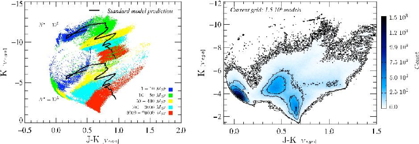
Figure 1: Stochastic properties of star clusters at solar metallicity. On the left panel, the dots represent photometric properties of individual clusters containing $10^{3}$ and $10^{5}$ stars each. The solid lines show the corresponding age sequences from “standard” predictions (Figure inspired by Bruzual (2002)). On the right panel, we show the corresponding density distribution of models in our main catalog, constructed assuming a power law with a index -2 for the cluster mass function. Note that the general aspect of this and subsequent model density maps will not change if the total number of clusters is increased, as required to extend the present study to higher cluster masses.

3 Analysis methods

The above synthetic populations can be used to analyse photometric observations of clusters. The properties we seek to estimate in this paper are the cluster ages and masses. We wish to account for the fact that observed colours can be affected by unknown amounts of extinction. Accounting for uncertainties in the metallicity is postponed.

In this section, we describe the Bayesian method developed for the analysis. Two other analysis methods are briefly described for comparison. One is a simple best-$\chi^{2}$ fit to all the data in the synthetic cluster catalog, the other is the usual estimate based on continuous population synthesis predictions. The comparison between results obtained with the three methods provides important insights into systematic effects.

3.1 Standard estimates: the “infinite limit”

The standard procedure implicitly considers the mass distribution of the stars in a cluster to be continuous. It has been applied widely, but as already mentioned, it is strictly valid only for populations of infinite mass. It becomes a reasonable approximation for clusters with masses above an age-dependent limit of about $5.10^{5}$ M_⊙. We include this method mainly to quantify the errors produced when it is applied to analyse the light of clusters of lower masses.

In families of spectra predicted with continuous models, mass is a simple scaling factor that applies to all fluxes. Therefore model spectra are frequently published scaled to a total population mass of $1$ M_⊙. Spectra are described only by age and extinction (and metallicity).

Assuming observational errors are Gaussian and independent, the most likely continuous model for a given set of broad-band fluxes is a minimum of the following function:

$$\chi^{2}_{\infty}=\sum_{k}\frac{\left(Y_{k}-M.Y_{k,\tilde{M_{\infty}}}\right)^{2}}{\sigma_{k}^{2}},$$ (1)

where $Y=\{Y_{k}\}_{k\in[1..n]}$ are the available data and the $\sigma_{k}$ the corresponding observational uncertainties. $Y_{k,\tilde{M}_{\infty}}$ are the fluxes predicted for the model $\tilde{M}_{\infty}$ (total mass $1$ M_⊙) and $M$ is the mass required to optimize the fit with this model.

We allow for extinction by looping through positive values of $A_{V}$ and repeating the optimization procedure.

3.2 Bayesian Estimates

As opposed to its continuous analogue, this approach explicitly accounts for the discrete and stochastic nature of the stellar populations. The cost in computation time is rather high, as the collections of synthetic clusters explored must be large (see Sect. 6.2.1).

As in all Bayesian approaches, the results are stated in probabilistic terms, and they depend on a priori probability distributions of some model parameters. In our case, the most probable ages and masses for a cluster, given a set of photometric observations, will depend on the age distribution and mass distribution of the synthetic clusters in the model catalog (the statement can be extended to include extinction and metallicity).

We assume observational errors are Gaussian with known standard deviations (a preliminary study of Lançon & Fouesneau (2009) used boxcar functions for the error distributions). An intrinsic model property $X$, for given photometric values $Y$, has the probability:

$$\mathcal{P}(X|Y)\propto\mathcal{P}(Y|X)\times\mathcal{P}(X).$$ (2)

Since errors are assumed to be Gaussian, the probability $\mathcal{P}(Y|X)$ can be expressed using the usual $\chi^{2}$ statistic:

$$\mathcal{P}(Y|X)\propto e^{-\chi^{2}/2}.$$ (3)

Then, the probability distribution of an intrinsic property, such as the age or mass of an individual cluster, is given by the following relation. The probability for property $X$ to be located in an interval $[x_{1},x_{2}]$, given photometric measurements $Y=\{Y_{k}\}_{k\in[1..n]}$ with uncertainties $\sigma_{k}$, is:

$$\mathcal{P}( X \in\ [x_{1},x_{2}]\ |\ Y)=\alpha$$ (4)

$$\times \sum_{\tilde{M}_{i}\,/\,X(\tilde{M_{i}})\in[x_{1},x_{2}]}\mathcal{P}(\tilde{M_{i}})\leavevmode\nobreak\ \prod_{k}\frac{1}{\sqrt{2\pi\sigma_{k}^{2}}}\leavevmode\nobreak\ e^{-\frac{\left(Y_{k}-Y_{k,\tilde{M}_{i}}\right)^{2}}{2\sigma_{k}^{2}}}.$$

In the above, $\alpha$ is the normalization constant (the value of which we calculate). The sum extends over all models that have an adequate value of $X$. $\mathcal{P}(\tilde{M}_{i})$ is the probability assigned to an individual model. Unlike the continuous models, the mass is an intrinsic parameter of each modelled population. As a first step, we consider all models in our main catalog equally probable, and therefore we inherit the distributions of age and mass used to construct the catalog. When we vary extinction, we consider flat probability distributions for $A_{V}$ between two boundaries. Through the factors $\mathcal{P}(\tilde{M}_{i})$, this expression of the probability can embody any prior mass or age distribution.

An analog of Eq. 4 can be written for joint probability distributions, for instance for age, mass and extinction. The most probable ages and masses given in this paper are the age and mass coordinates of the maximum of the joint distribution. Error bars can be given by examining all models above a given probability threshold.

In our main catalog, as we mentioned before, the prior mass function is a power law with an index $-2$, and log(age) is distributed uniformly (above $50$ Myr). Clearly, it will be necessary to investigate the effects of these assumptions quantitatively, by varying them within reasonable limits. Due to the above described catalog mass completeness limit, we postpone this study to a future work.

3.3 Single best fit

As a simple first step towards accounting for stochastic fluctuations, one may look at the one model in the catalog that minimizes the standard $\chi^{2}$ function

$$\chi^{2}_{i}=\sum_{k}\frac{\left(Y_{k}-Y_{k,\tilde{M}_{i}}\right)^{2}}{\sigma_{k}^{2}}.$$ (5)

4 Analysis of UBVIK photometry

As a first study, we compare the results from the three methods above in the joint analysis of U, B, V, I and K band fluxes. The analysis is applied to the synthetic absolute magnitudes of a subsample of clusters from our main catalog. The presentation is twofold: in Sect. 4.2 and 4.3 the synthetic magnitudes are used unchanged, while in Sect. 4.4 noise is added before the analysis is performed.

4.1 Input sample description

The comparison of mass and age estimates is presented for clusters with relatively small masses, where our catalog is most complete and where the effects of stochasticity are most important. Figure 2 shows the mass-age distribution of our input sample. It contains 1000 models randomly selected from our main MC catalog. It covers a relatively small mass range, but a broad range of ages (though mostly above $10$ Myr). The model colours are not reddened (unless otherwise stated) and the model cluster distances are set to $10$ pc – the observable properties associated with the models are absolute magnitudes or fluxes. Note that the selected sample reflects the intrinsic prior mass and age distributions of the catalog.

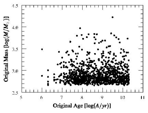
Figure 2: Model sample from our main MC catalog. 1000 models were randomly extracted from the catalog in order to identify systematics. Selected clusters are low mass populations and cover a broad range of ages. Fluxes are not reddened and calibrated as absolute fluxes, corresponding to a $10$ pc distance.

4.2 Estimates from photometry without noise

The estimates of age and mass obtained from the synthetic data with the standard method and with the stochastic Bayesian method are shown in Fig. 3. Estimates from the single best fit method are not shown, as this method returns the input model itself when no noise is added to the synthetic data. The standard deviations in the above equations (1), (4) and (5) are set arbitrarily to 0.05 magnitudes. In this first experiment, the absence of extinction, is considered to be known to the “observer”. This could be constrained for instance with emission line measurements or with estimations of the total gas content of the host galaxy. The alternative experiment, where the extinction is a free parameter of the analysis is described in Sect. 4.3.

4.2.1 Biases in the estimates from the standard method

The bottom panels of Fig. 3 reveal the inadequacy of continuous population synthesis models for the analysis of the colours of realistic clusters of small masses.

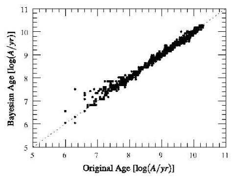
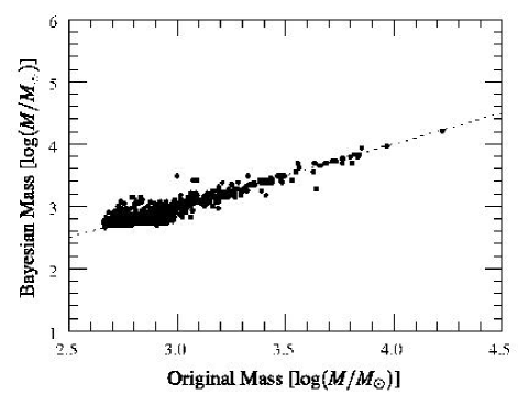
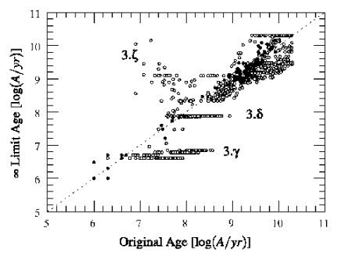
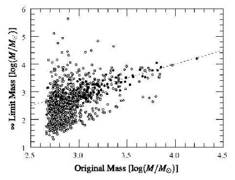
Figure 3: Estimations based on U, B, V, I and K band fluxes without noise, when assuming no extinction (A${}_{V}=0$, “true” value). Estimations from the Bayesian approach are given in the two upper panels and standard estimation considering an infinite number of stars are given in the two lower panels. The x-axes represent, respectively, the original age and mass of the sampled populations whereas the y-axes represent the estimated values from the two methods. Dashed lines highlight the identity function. Labels are referenced features within the text. Open circles highlight poor fits where the reduced $\chi^{2}$-values are larger than $3\sigma$ confidence range, standard deviation of the $\chi^{2}$-law.

The fits to the UBVIK data are poor. $93$% of the $\chi^{2}$ values are more than 3$\sigma$ above the value expected for a good fit if one assumes observational errors of 0.05 magnitudes ($\sigma$ refers to the standard deviation of a $\chi^{2}$-law with 3 degrees of freedom). In other words, no statistically acceptable match is found in most cases.

Cluster ages are typically underestimated, with a few exceptions. Errors of $1$ or even $2$ dex are not rare. As a consequence, mass estimates are highly dispersed. And if one fails to reject clusters with poor fits, the masses are on average underestimated by $0.3$ to $0.5$ dex.

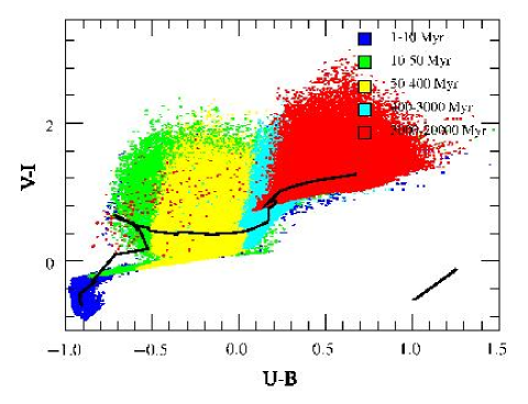
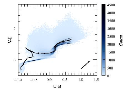
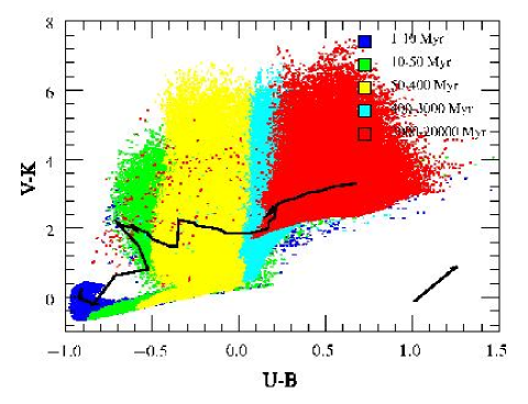
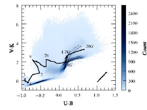
Figure 4: Photometric properties of stochastic populations compared to average predictions at solar metallicity. On the left hand panels, the dots represent coulours of individual clusters contained in our MC catalog. Note that there are large regions of overlap between age bins, and that older models hide younger models in certain areas of the figure. The extinction vector is given by the arrows assuming a Cardelli extinction law (Cardelli, Clayton, & Mathis, 1989). On the right panels, the corresponding density distributions of the models are shown, assuming cluster masses follow a power law with an index -2. The solid lines represent the corresponding age sequences from “standard” predictions. Numeric labels on the bottom left panel correspond to the age sequence from $1$ Myr to $20$ Gyr. Dotted lines emphasize high density regions mentioned in Sect. 4.2.

Fig 4 helps us understand why derived ages tend to concentrate around $5-9$ Myr and $80-100$ Myr, in features that we labeled 3$.\delta$ and 3$.\gamma$ in Fig. 3, leaving gaps at other ages. We note that this remarkable effect is seen in many cluster mass distributions presented in the literature (e.g. Gieles, 2009) and has received partial explanations (e.g. Fall, Chandar, & Whitmore, 2005).

Since there is no extinction, the optimization will simply search for the nearest continuous model in the UBVIK-space. For intermediate age clusters, hooks in the locus of continuous models make individual ages more or less attractive. For instance, the supergiant evolution phase, which occurs around $9$ Myr in our models, is very attractive and translates into the feature 3$.\gamma$ in Fig. 3. The accumulation around $100$ Myr (feature 3$.\delta$) results from the redward excursion of V$-$K when the upper Asymptotic Giant Branch (AGB) first becomes populated. The attractive effect of these particular points is enforced by the fact that the spread of the models is significantly wider in V$-$I compared to U$-$B (Fig.4): moving across wide parts of the distribution in U$-$B has a lower cost in terms of $\chi^{2}$ variations than moving along U$-$B.

Although in most cases the best $\chi^{2}$ values are not statistically acceptable (again statistically $93$% of the input-clusters are not well fitted), the match nevertheless provides a decent age for relatively old populations.

Finally, objects containing more luminous stars than the continuous models, tend to be very red. With no extinction, this leads to overestimates of the population ages, which produces feature 3$.\zeta$ on Fig. 3.

Typically, young continuous models are more luminous, per unit mass, than older ones. Hence any trend in the age estimates will translate into the equivalent effect on the derived masses. Therefore, this method tends to also underestimate masses of small clusters.

4.2.2 Bayesian estimates

Unlike the standard method, the Bayesian analysis based on stochastic cluster catalogs returns ages and masses in excellent agreement with the input values as shown by the top panels of Fig. 3. As already mentioned, the single best fit model is exactly the model used to synthesize the photometry for the analysis. Shown here are the most probable model properties, after a Bayesian analysis that assumes observational errors of 0.05 magnitudes (although no noise was actually added to the input photometry).

The masses assigned with the Bayesian method are distributed symmetrically around the input values, except for a cut-off at $500$ M_⊙ due to the low-mass limit of our cluster catalog. About $20$% of the analysed clusters are potentially affected by this limit.

The standard deviation of the residuals are of $0.1$ dex in age above $20$ Myr and $0.08$ dex in mass above $10^{3}$ M_⊙ (the age and mass lower limits are set to avoid statistical biases due to the current limitations of our MC-catalog).

4.3 When extinction is a free parameter

In the previous section, cluster colours were analysed by comparison with models during which the amount of reddening imposed to be null in the optimisation.

We have shown that in most of cases the standard analysis method leads to under-estimated ages, and masses, even with high quality photometric data across the spectrum from U to K. The fraction of clusters with underestimated ages was significantly reduced when adopting stochastic models rather than the classical continuous ones.

We now assume that no independent information on extinction is available to the “observer”. Hence for the analysis we allow the extinction, $A_{V}$, to vary between $0$ and $3$ with steps of $0.2$.

Figure 5 shows the results obtained when repeating the analysis of the reddening-free sample of Sect. 4.1, this time authorizing any reddening of the models. The colours of a reddened sample are analysed in Sect. 4.3.3.

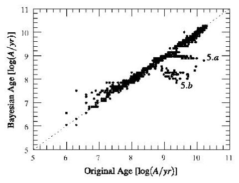
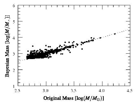
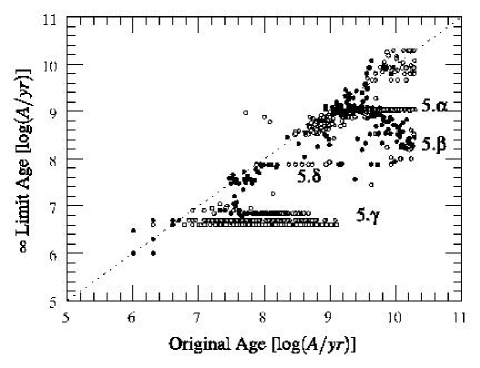
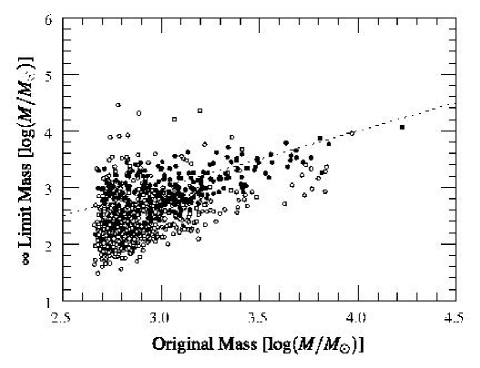
Figure 5: Estimates based on U, B, V, I and K band fluxes without noise, allowing an extinction A_V from $0$ to $3$. The conventions and axis significations are the same as Fig. 3. On the left-hand side, the age estimations. On the right-hand side, the mass estimations.

4.3.1 Estimates from the standard method

The bottom panels of Fig. 5 confirms the inadequacy of continuous population models for the analysis of realistic clusters of small masses. By authorizing the extinction to vary, we do increase the fraction of clusters whose colours can be fitted satisfactorily with continuous models, but only to $22$ %.

Again assigned ages are highly clustered, and most of them are underestimated. As a consequence, mass estimates are highly dispersed.

In the standard method, dereddening is the only cost-free way, in terms of $\chi^{2}$, to move an observed cluster to the line representing the continuous models. If we look at the UBVI or UBVK colour-colour planes shown on Fig. 4 (left panels), the reddening vector is almost orthogonal to the loci of stochastic clusters of constant age. Recall that the input sample is drawn from the stochastic collection even if it is analysed with the continuous models. Dereddening therefore leads to underestimated ages.

Derived ages tend to concentrate around around $5-9$ Myr, $80-100$ Myr and also $1$ Gyr, figures that are labeled 5$.\alpha$, 5$.\beta$ and 5$.\gamma$ in Fig. 5. Using the direction of the extinction vector in Fig. 4 and starting from the bending points of the line of continuous models, one can define large areas of the colour-colour planes in which all clusters will be assigned the same ages (with fits of medium or poor quality). For instance, all clusters with $-0.5<$U$-$B$<0.3$ and V$-$K$<1.5$ (or V$-$I$<0.2$) (clusters in the yellow or blue age bins and below the continuous model line) will be assigned ages of $5-7$ Myr, which causes feature 5$.\gamma$, very similar to the previously described 3$.\gamma$. Old clusters are preferentially located on two branches of high model density in our (prior dependent) MC-model collection. Those two regions, emphasized by the dotted lines on the right panels of Fig. 4, are crossing each other around U$-$B$=0$. Clusters in the lower branch, with the higher model density (at V$-$K$\sim 2$), will be assigned an age of $1$ Gyr and produce feature 5$.\alpha$. The older of these will be assigned higher extinction values. Clusters near the second and more diagonal branch (V$-$K$>2.5$) will be assigned ages between $100$ Myr and $1$ Gyr, with a systematic trend towards younger ages for redder, older clusters (feature 5$.\beta$). Note that the accumulation 3$.\delta$, described previously, is still present but weaker. Feature 3$.\zeta$ has disappeared.

Again, young continuous models are typically more luminous, per unit mass, than older ones. In most cases, this age effect is stronger than the luminosity variation associated with the dereddening procedure. Therefore, obtained masses are usually smaller than the actual masses. There are exceptions however, for clusters associated with large estimated (i.e. overestimated) amounts of extinction.

4.3.2 Bayesian estimates

Despite the additional degree of freedom associated with extinction, the Bayesian analysis based on stochastic cluster catalogs generally returns ages and masses in good agreement with the input values (top panels of Fig. 5).

Above $20$ Myr, $90$ % of the most probable ages lie within $0.3$ dex of the actual age (r.m.s. dispersion of $0.1$ dex). For the remaining $10$% of the clusters in the sample, the age estimates present attraction points again, and this leads to underestimates of up to $1.5$ dex. The favoured ages are located just below $1$ Gyr and around $100$ Myr. The corresponding features are labeled $3.a$ and $3.b$ in Fig. 5. While their locations are not far from those of $3.\alpha$ and $3.\beta$, their origins are different.

The Bayesian “attractors” are regions of high concentration in the model density plots of the right panels of Fig. 4. They do not lie along the locus of continuous population synthesis models. Since all models with magnitudes within about 0.05 of the observations are given large weights in the computation of the posterior probability distribution, areas of high model density along the dereddening line are favoured. An illustration is provided in Fig. 14 and discussed further in Sect. 6.2. The clusters affected by this issue are usually located in regions of low model density of the colour-colour and colour-magnitude planes; they are assigned positive extinction values.

4.3.3 Reddened input clusters

As the extinction seems to play a role in the resulting trends of derived ages and masses from integrated photometry analyses, we conduct the same experiment as before, where the input sample photometric dataset was reddened by a factor of $1$ optical magnitude, assuming a Cardelli extinction law (Cardelli, Clayton, & Mathis, 1989).

Fig. 6 presents the resulting age and mass distributions of the derived properties when using the Bayesian method. $97$% of the clusters have a correct derived extinction of $1$ mag according to the Bayesian estimates. The standard deviations of the residuals are of $0.2$ dex in age above $20$ Myr and $0.1$ dex in mass above $10^{3}$ M_⊙. Trend features presented on Fig. 6 are very similar to the previously mentioned ones. A few clusters now have overestimated ages, because reddening has moved them from the blue side to the red side of a region of high model density and typically older ages. This region of high model density becomes a Bayesian attractor for these reddened clusters, while it was out of bounds in the reddening-free case (reaching this region of high model density would have required negative extinction corrections).

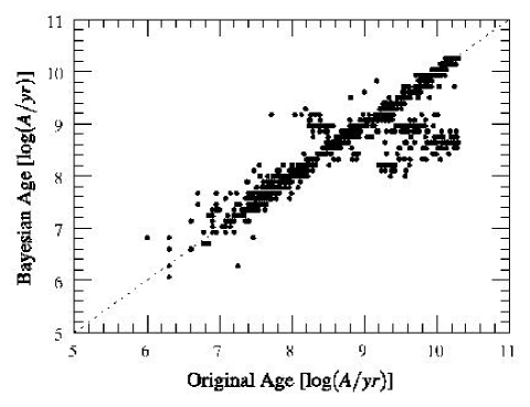
Figure 6: Derived age (left) and mass (right) distributions using Bayesian method analysing UBVIK data when $1$ mag extinction (assuming Cardelli extinction law) is applied to the input population properties. This figure compares directly with Fig. 5.

4.4 Estimates from noisy fluxes

We now reproduce the analysis of Sect. 4.3 for the same inputs, but after having added Gaussian noise to the input fluxes ($5$ %). Figure 7 presents the results. At the top of this figure are also plotted estimates derived from the single best-$\chi^{2}$ fit.

Although the inputs are now noisy, the trends obtained remain similar. In particular, there is no important difference with the noise-free case when the analysis is based on standard, continuous population synthesis models (bottom panels): most fits are poor, ages tend to be underestimated, masses are highly dispersed around the correct values.

Bayesian estimates remain close to the expected values even though the dispersion has increased. The standard deviation of the residuals are of $0.15$ dex in age and $0.13$ dex in mass except for models in $6.a$ and $6.b$ features. Only $13$ % of the model clusters are assigned underestimated ages.

A pleasant fact is that the single best-$\chi^{2}$ fit provides results that are similar to the Bayesian ones (see discussion in Sec. 6.2.1). Although individual clusters are assigned different ages, the estimated properties of the sample as a whole are described similarly with both methods. For 84 % of the clusters, the single best fit age and the Bayesian ages are both within $0.3$ dex of the actual ages. Of the 16 % that deviate, 3 % deviate only with the single best fit method, 3 % only with the full Bayesian method, and 10 % deviate in similar ways with both methods.

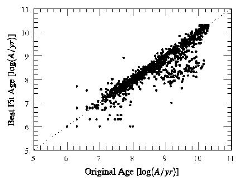
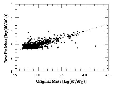
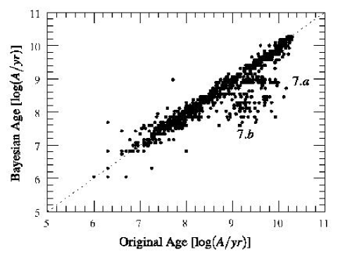
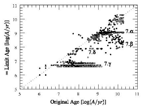
Figure 7: Estimations based on U, B, V, I and K band fluxes with 5% noise added to the photometry inputs, allowing an extinction A_V from $0$ to $3$. From top to bottom, the direct fit of the noised populations by our catalog, the Bayesian estimations and the standard estimations. The conventions and axis significations are the same as Fig. 5.

5 When there is no K band data

It is common understanding that near-IR light is a better tracer of mass in galaxies than optical light, and that including near-IR photometry helps break degeneracies and estimate ages. Particularly illustrative figures on the latter point can be found in Bridžius et al. (2008). However, all these statements rest on models that are valid only in the limit of large numbers of stars, i.e. not for most of the real star clusters in the Universe. This Section re-assesses the role of photometry beyond wavelengths of $1\leavevmode\nobreak\ \mu$m in the stochastic context appropriate for small clusters.

Figure 8 shows the results obtained for the sample of Sect. 4.1 when using noise-free UBVI input fluxes. Extinction is a free parameter although, as above, the clusters analysed are not reddened. Figure 8 compares directly to Fig. 5.

With a smaller number of observational constraints, it is much easier to obtain statistically acceptable $\chi^{2}$ values. $80$ % of the clusters in the sample now find an acceptable match among the standard, continuous population synthesis models (with extinction when convenient).

A very unusual result is that between about $10^{8}$ and $10^{9}$ yr the standard method (based on continuous models) produces better ages when the K data is absent than when it is present. This is due to the relative locations of the line of continuous models and the regions of high model densities, in colour space (Fig. 4). At intermediate ages the offset is of one full magnitude in $(\mathrm{V}-\mathrm{K})$, whereas it remains small in other colours. For a cluster that is typically located in the high density region, the nearest continuous model will produce a decent $\chi^{2}$ without need for much reddening in UBVI but large $\chi^{2}$ values in UBVIK. The rare but luminous AGB stars strongly increase the impact of stochasticity on the derived properties so that one should think about throwing K band data away when the UBVI-estimated age is between $100$ and $500$ Myr.

At other ages, the standard method applied to UBVI fluxes shows artefacts: a very strong accumulation is found at estimated ages around $1$ Gyr, and hardly any cluster is assigned ages between $2$ and $7$ Gyr. But these artefacts are not much worse than those seen in the analysis of UBVIK data with continuous models.

In terms of estimated masses, the distributions around the correct values are similar whether one uses UBVI or UBVIK data as input to the standard method (continuous population synthesis). On average, the masses of the clusters for which the UBVI fit is satisfactory are underestimated slightly ($0.2$ dex at $10^{3}$ M_⊙).

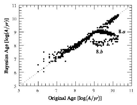
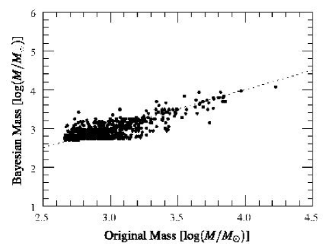
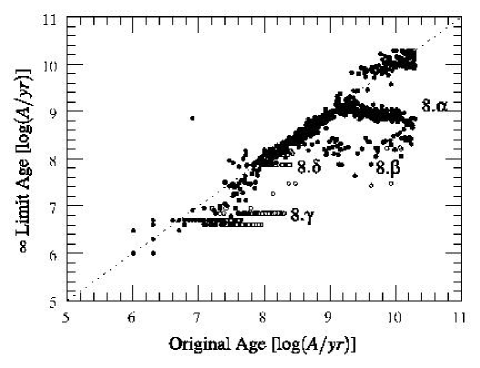
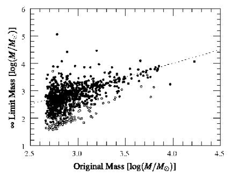
Figure 8: Same figure as Fig. 5 but excluding information on K band: estimations are based on U, B, V, I bands without noise, allowing an extinction A_V from $0$ to $3$. This Figure compares directly to Fig. 5.

When using the Bayesian analysis based on stochastic models, the loss of the K band information translates into stronger artefacts in the derived age distributions. The model-density distribution in colour space plays a more important role in Eq. (4) when there is less contrast in the $\chi^{2}$ distribution, i.e. when K fluxes are absent. Ages in high density regions along the de-reddening lines become more attractive. Note that these artefacts disappear if the amount of reddening is known rather than being a free parameter.

The artefacts in the age distributions of the standard and the stochastic method, without the K band, appear oddly similar (left panels of Fig. 8). In fact, the clusters in features $7.b$ and $7.\beta$ are mostly identical, while the clusters in features $7.a$ and $7.\alpha$ form two subsets with very little overlap.

One must distinguish three main behaviours for clusters that have ages between $1$ and $10$ Gyr. Feature $7.\alpha$ is due to the clusters located in the main high-density region of model colour-space, i.e. the region that runs parallel to the line of old continuous models in the lower right panel of Fig. 4 but is not superimposed on that line. These clusters will be assigned correct ages with the Bayesian method, but an age around $1$ Gyr (and a positive extinction) with the standard method. Feature $7.a$ is due to clusters located in the secondary high-density region of colour-space, which happens to be superimposed on the line of old continuous models (when there is no K band data). These clusters will be assigned correct ages with the standard method, but will be attracted to younger ages with the Bayesian method (with a positive extinction) because of the contrast in the model-density maps. Finally, the rarer clusters with larger than typical $V-I$ colours will be attracted to ages around $100$ Myr (with a positive extinction), both with the standard and the Bayesian methods (features $7.b$ and $7.\beta$).

As noted earlier, underestimated ages lead to underestimated masses because stellar populations fade with time and extinction corrections do not quite compensate for this. In our sample, many of the old clusters affected by the age artefacts get assigned masses near the lower limit ($500$ M_⊙) of our catalog (see Sect. 6.2).

Outside the main age artefacts seen for old clusters (when extinction is a free parameter), the Bayesian methods recovers ages and masses similarly well whether or not the K band fluxes are included in the input data. If we exclude objects lying in the features $7.a$ and $7.b$ as well as objects affected by the low-mass limit of our MC catalog, masses recovered with UBVI data sets are not significantly more dispersed ($\sigma=0.14$) than those obtained with UBVIK data sets ($\sigma=0.13$). Further aspects of photometric band-pass selection are discussed in Sect. 6.3.

6 Discussion

Several decades have passed since the stochasticity of stellar populations was first mentioned (Barbaro & Bertelli, 1977) as a serious issue. With powerful computers, stochasticity can now be taken into account explicitly when analysing the properties of unresolved populations.

Considering stellar populations as stochastic requires some changes in habits, for instance because mass is not a simple scaling factor anymore: errors on absolute fluxes (e.g. due to uncertainties on distances) can affect estimated ages; and observations of only colours can provide some information on the mass. Clearly, more work is needed to explore the consequences of stochasticity more exhaustively.

6.1 Non-stochastic studies : mass and age distributions

The analysis of the integrated light of small clusters with continuous population synthesis models produces strong age-dependent artefacts in the derived ages, and a broad distribution of random errors in the derived masses.

The good news is that there is no large systematic offset between estimated and real masses if the photometric data are of good quality and if observations that cannot find a statistically acceptable match among the continuous models are rejected. When the data have larger errors, fewer model fits are rejected. Then, a systematic trend appears in addition to the random errors: masses are underestimated on average. The value of the offset depends on the photometric pass-bands available and on the existence (or not) of independent information on extinction. The average error is of $0.3$ dex for a sample of clusters of masses around $10^{3}$ M_⊙ observed in UBVIK, when extinction is treated as a free parameter.

The above means that mass distributions of large samples of clusters based on an analysis with continuous population synthesis models are probably not too strongly biased. Several empirical determinations in the literature (see Rafelski & Zaritsky, 2005, and references therein) favour $M^{-2}$ mass distributions, and we used such a law as a prior in our Bayesian analysis. We find no immediate reason to apply a correction to this result, although a detailed investigation of each individual dataset in the literature would be worthwhile. If, for instance, small masses are systematically underestimated by $0.3$ dex while large masses are not, the power law index of the mass distribution would require a small correction.

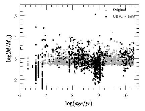
Figure 9: Age-mass and age-luminosity distributions obtained for our test sample, when analysing UBVI data with standard, continuous population synthesis models. Grey dots represent the test-sample and black ones the recovered properties. In the right panel, masses have been converted to luminosities using the (continuous) mass-to-light ratio given by Pégase (solid line: $10^{3}$ M_⊙ cluster).

Figure 9 shows the age-mass distribution obtained when UBVI data for our test sample of clusters is analysed with non-stochastic population synthesis models and no fit is rejected. While the properties of the test sample are smoothly distributed, the estimated properties are highly clustered. The figure looks similar with UBVIK data, but we chose UBVI for comparison with the (UBVI+H$\alpha$)-based age-luminosity distribution of (more massive) Antennae clusters (Fall, Chandar, & Whitmore, 2005). The right panel of Fig. 9 shows the derived distribution in the age-luminosity plane, after conversion of the estimated masses into luminosities with the age-dependent mass-to-light ratio given by Pégase. In an observational context, such a figure would be truncated at low luminosity by some instrumental sensitivity limit.

The similarity between the distribution in Fig. 9 and that in Fig. $1$ of Fall, Chandar, & Whitmore (2005) is striking, even more so when one mentally corrects for the sharp low-mass limit of our sample and our relative lack of young clusters. Accumulations and gaps occur at essentially the same ages (differences can be traced back to the different sets of evolutionary tracks used by the authors). We have discussed the origins of the artefacts in our test-sample age distribution in Sect. 4: they arise because real, stochastic clusters of small masses are distributed over a wide range of colours, and can therefore fall quite far off on the line of continuous models when only extinction is available to alter their colours. The clusters in the Antennae sample, however, are typically 50 times more luminous than the ones in our study. More massive clusters should lie closer to the lines of continuous models. Why then are these artefacts so strongly seen in the Antennae cluster distribution? Our interpretation is that the combined effects of observational errors and real extinction disperse the clusters enough in colour-space to produce a global derived age distribution that is similar to the distribution produced at lower masses by stochasticity.

The input age distribution of the clusters in our test-sample (and in our main MC catalog of clusters) is constant in logarithmic age bins, and this produces derived age-luminosity distributions that are very similar to the ones in the literature. Our tentative conclusion is that the adopted age-distribution is, for the time being, an adequate prior for the Bayesian, stochastic studies. Clearly, it would be desirable to explore quantitatively how sensitive the derived distributions are to the actual age and mass distributions, especially in the presence of observational errors. Any firm conclusion on the Antennae clusters, for instance, would require such a study.

6.2 Prospects of the stochastic analysis

The analysis of cluster colours based on a library of stochastic models provides ages and masses with small random errors, and with systematics that will be negligible in many situations.

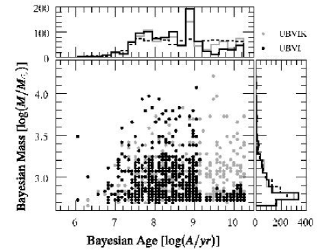
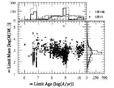
Figure 10: Resulting age-mass distributions from the Bayesian (left panel) and standard (right panel) analysis methods on the test-sample clusters. Grey dots are estimates from UBVIK bands whereas black dots are from UBVI bands only. UBVIK distribution on the right panel is presented in left panel of Fig. 9. Note that binning effects are visible on the Bayesian distribution as mentioned in the Sect. 6.2. The original age-mass distribution is presented on Fig. 2.

Figure 10 shows the derived age-mass distributions for our test sample, based on either UBVI or UBVIK data sets. Similar results are obtained if the input sample is reddened (Fig. 11). The situation can be improved even more if there are independent constraints on extinction.

The figures show the grid pattern due to the finite sizes of our bins in estimated ages and masses. This is because we compute the posterior probabilities of Eq. 4 for finite intervals.

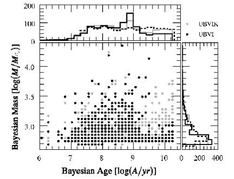
Figure 11: Resulting age-mass distributions from the Bayesian analysis methods on the $1$-mag reddened test-sample clusters. Grey dots are estimates from UBVIK bands whereas black dots are from UBVI bands only. Corresponding marginal distribution histograms follow the same color conventions. The dotted line on the histograms represent the test-sample distribution.

The binning procedure has a caveat and an advantage. The caveat is that results are sometimes sensitive to the choice of the bin sizes or boundaries. We have looked at many probability maps in 2D projections of age-mass-extinction space to check where this occurs. Examples are given in Appendix A (all can not be developed here). As expected, the results are robust with respect to the binning (i.e. errors are smaller than or equal to one bin size) when the maps are simple, single peaked (Fig. 13), while they can depend strongly on binning when the maps are complex (i.e. in cases in which uncertainty estimates based on contours of equal probability would give large error bars). The second type of situation occurs especially when there is no a priori information on extinction. Figure 14 illustrates this event: the dereddening vector of an object crosses several regions of high model-density. The model properties within each of these regions end up with similar probabilities. Which one dominates, depends on the binning as shown on Fig. 15 (and on the density pattern itself).

The advantage of binning is that we can, to first order, assign the ages, metallicities and extinction of a given bin the same a priori probabilities. This allows us to rescale the derived probability maps for a cluster after calculation, if we wish to change the adopted priors (a worthwhile gain in computation time). In our current catalog, the total number of clusters with masses above about $10^{4}$ M_⊙ is too small to allow us to study flatter mass distributions of clusters immediately, and we also lack clusters with ages below $10^{7}$ yr. We have therefore chosen to postpone the description of consequences of changes in the priors to a future article.

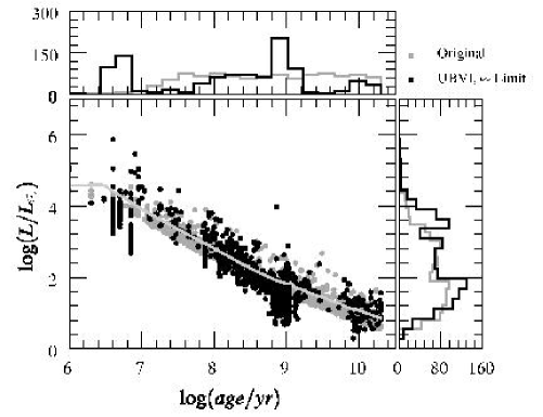
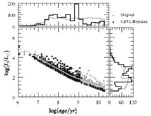
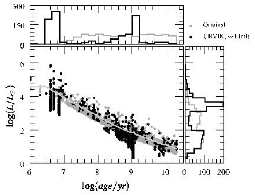
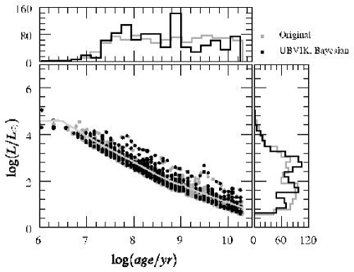
Figure 12: Age–luminosity recovered distributions obtained for our test-sample. Grey dots are the original distributions and black dots are respectively the recovered distributions from the standard (left panels) and Bayesian (right panels) methods when analysing UBVI (top panels) and UBVIK (bottom panels) data sets. Recovered masses are converted to luminosities using Pégase (continuous) factor of which the solid lines represent the evolution of a $10^{3}$ M_⊙ cluster.

6.2.1 Other practical aspects

Although conceptually simple, the implementation of the Bayesian, stochastic analysis is not immediate. Constructing the stochastic library requires CPU time and data storage. For each cluster, the spectra of at least the brightest 1000 stars need to be summed individually. The remaining low mass stars could be represented with a continuous sequence to save computation time. Synthetic broad band colours can then be measured on the resulting total spectrum. We decided to save all the spectra and to compute a set of 60 standard broad band fluxes (standard UBVRIJHK, but also most HST filters and some from other telescopes). For three metallicities and several millions of models in total, the computation took a couple of month on six $3$ GHz CPUs, and half a terabyte of data was accumulated.

Browsing through the collection to compute probabilities also takes time, even with the restriction to a few photometric bands. A few CPU-hours are required to construct probability distributions of age, mass and extinction for $1000$ clusters with our main MC catalog, allowing for extinction to vary in the range described above. It is somewhat faster to use a simple best-$\chi^{2}$. This may be good enough for statistical studies of large samples, but it must be kept in mind that the single best fit can be far from the Bayesian most probable model in individual cases. Very small changes in the observed colours (due to small observational errors) can modify single best fit parameters, while they leave Bayesian estimates unchanged. To provide error bars on the single best fit parameters, one has to explore the vicinity of the minimum $\chi^{2}$. For instance, one could compare the properties of all the models with a $\chi^{2}$ below a predefined threshold, as was done for large clusters in Bridžius et al. (2008) or Anders et al. (2004). Doing this exhaustively would be conceptually similar, and essentially as long to run, as our Bayesian approach.

All the results in this paper are based on one single set of population synthesis models. Some caveats of these models are that they do not include the formation of carbon stars or Mira-type variability, and that they do not account for binaries or for stellar rotation. We have not yet compared the amplitude of the errors arising from stochasticity (studied here) with those due to uncertainties in the physical assumptions of the models. However, we expect qualitatively similar systematics with any set of stellar evolution tracks. It will unfortunately be necessary to recompute a completely new library if one wishes to explore different sets of stellar evolution tracks, to assume a different stellar mass function, or to use a different library of stellar spectra. This will clearly limit the pace at which the comparisons can be made.

6.3 Impact of the photometric band selections

In the present paper, the estimation of ages and masses has been shown to be affected by stochasticity and also by the photometric datasets used during the analysis. We chose to focus on explaining behaviours rather than multiplying experiments with different pass-bands, and have therefore restricted our quantitative comparisons to two combinations. In a large fraction of stellar population studies, the UBVI combination is used as the standard selection: it provides a reasonable compromise between depth and spectral coverage for most of the available instruments. Moreover, it corresponds to a wavelength range where spectral libraries are the most accurate. Adding the K band improves mass estimates in the non-stochastic regime of high total masses, but it has an observational cost as it requires the use of a different instrument. Testing the UBVIK combination in the stochastic regime provides useful information for the design of future surveys.

In Sect. 5, we presented some effects of the presence of K band data in addition to UBVI photometry. The K band does not improve significantly the situation when continuous models are being used (right panel on Fig. 10). In particular, we mentioned that including the K band in the analysis of populations with AGB stars ($100-500$ Myr) may lead to even worse estimates (again with continuous models). This effect is also visible on the left-hand side panels of Fig. 12. On the other hand, we found only mild improvements when including K band data in the Bayesian analysis: the presence of K band information translates into weaker artefacts in the derived age distributions (artefacts which disappear when reddening is not a free parameter). The left panel of Fig. 10 presents recovered age-mass distributions for UBVI and UBVIK datasets using the Bayesian approach, with free extinction. Old populations ($>1$ Gyr) age-mass estimates reflect the original distribution better when K band constraints are included. This is also visible on the right panels of Fig. 12, where the resulting distributions are significantly improved.

At young ages, both our test sample and our main MC catalog are underpopulated. Most small and young clusters have HR diagrams that resemble a truncated main sequence. Even if the stellar mass function from which their stars are drawn randomly extends to 120 M_⊙, a small zero age cluster will in general contain zero ionizing stars, and a small cluster aged 10 Myr will contain zero red supergiants : two such objects are basically indistinguishable, be it with or without K band data. This problem shows up clearly when we run the Bayesian analysis at young ages, but quantifying this effect requires that we add more young clusters to our reference catalog.

The UV spectral range raises questions similar to the near-infrared. We repeated some of the above experiments with UBVI and the F218W filter, centered around $220$ nm (WFPC2 instrument on-board the Hubble Space Telescope). A brief summary is that the effects of adding this UV band have amplitudes similar to those obtained when adding K. The dispersions in the results are comparable to those without UV, both for Bayesian or standard estimates. Artefacts are also qualitatively similar. Age estimates below $20$ Myr are improved only slightly.

If one however wants to include UV bands, the choice of an extinction law becomes more of an issue. Extinction laws indeed express a range of behaviours in the UV bands (e.g Allen, 1976; Fitzpatrick & Massa, 1986; Cardelli, Clayton, & Mathis, 1989; Calzetti et al., 2000).

The decision of which filters to use rests on considerations of the astrophysical problem to tackle. Using either UV or K photometry does not deeply affect the resulting estimates ages and masses of small clusters. One may first want to consider using discrete population models instead of continuous ones.

7 Conclusions

Studies of star cluster populations in galaxies have been based until now on continuous population synthesis models, that provide a very poor approximation of the integrated light of clusters of small and intermediate masses because this light is determined by a very small number of luminous stars.

Based on large collections of Monte-Carlo simulations of star clusters that each contain a finite number of stars, this paper explores systematic errors that occur when the integrated fluxes of realistic clusters of small masses are analysed in terms of mass and age. Our main collection is built with the cluster age and mass distributions of Fall, Chandar, & Whitmore (2009), extrapolated to masses lower than those observed in the Antennae galaxies.

With the standard methods (continuous models), large systematic errors affect estimated ages and large random errors affect masses. If observational uncertainties on cluster fluxes are large and, as a consequence, quality-of-fit criteria fail to reject the numerous poor fits, systematic errors (of a few tenths of a dex) are also present in the estimated masses. Derived age-mass or age-luminosity distributions for samples in which actual ages and masses are distributed as in our main collection display clustered patterns that very closely resemble those found in empirical samples in the current literature. We find no immediately obvious reason to reject the age and mass distributions of our main collection, but clearly this essential point requires detailed study with real observations.

A Bayesian method has been described and implemented, in order to account explicitly for the finite nature of clusters in the analysis. It is shown that their age and mass can be recovered with error bars that will be small enough for many purposes. Young small mass clusters will remain difficult to age-date because HR-diagrams of many of them identically look like truncated main sequences with no ionizing or post-main sequence stars. At intermediate ages, the variability of luminous AGB stars is expected to cause difficulties that we have not yet solved.

The comparison between the results obtained with UBVI and UBVIK data sets shows that, in the stochastic context, the benefits of adding the K band to optical observations are rather small, except for the mass determination of clusters older than 1 Gyr. Clearly, adding near-IR or UV information is secondary, compared to the need to move from continuous to stochastic cluster models.

The Bayesian analysis method can now be applied to existing data on cluster samples in nearby galaxies with the aim of constraining the actual age and mass distributions of these clusters. We will also extend the study of systematic errors to the case where metallicity is an unknown parameter.

Appendix A Examples of probability maps

The method we developed to take the stochasticity into account to estimate intrinsic parameters (age, total number of stars or total mass, metallicity, extinction) of unresolved population follows a Bayesian approach. Given a set of photometric measurements and uncertainties, we establish the joint probability distributions of these parameters based on a large catalog of Monte-Carlo simulations. In this appendix, we present examples of probability distributions.

First an example is given on Fig. 13, for which we obtain single peaked probability distributions leading to an unambiguous probabilistic determination of age, mass and extinction estimates. In this example, we recover that the most likely have no extinction and the most probable age and mass are $35$ Myr and $630$ M_⊙, very close to the expected values.

As we discussed in Sect. 6.2, it also happens that the probability distributions are not single peaked. Complex maps occur when there is no independent known information on the amount of extinction. Figure 14 illustrates how the extinction factor increases the complexity of the probability maps. The top-left panel contours show how the color distributions are affected along the dereddening vector. On this example, the object crosses three regions of high model density. The resulting age-mass probability distribution is multi-modal (trimodal).

Complex distributions are subject to binning issues. The example probability distributions given on Fig. 14 yields three modes with similar probabilities. If one changes the number of bins on which the probabilities are computed, peak values might vary to eventually change the dominant mode of the distributions. The Figure 15 shows that the variations of the resulting age estimates can be significant: from $2.3$ Gyr to $50$ Myr . A determination of the optimal binning remains an open issue.

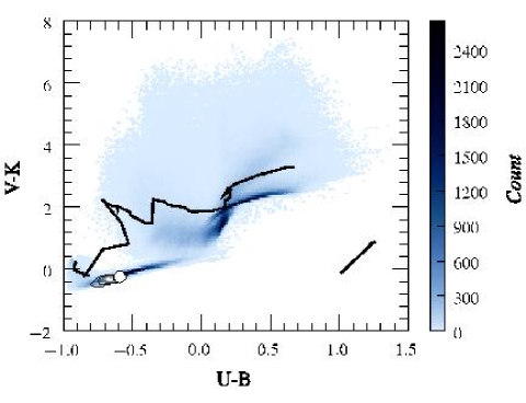
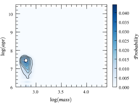
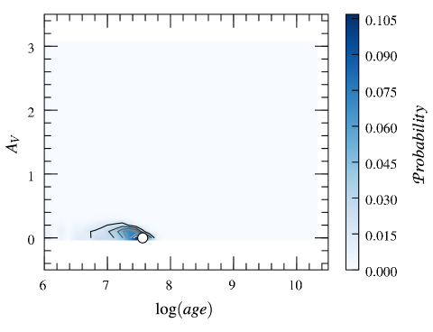
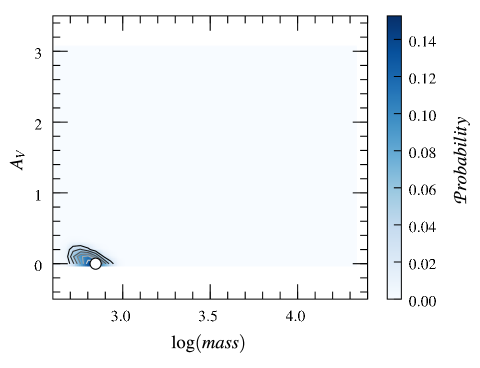
Figure 13: Example of probability map for a population of $33$ Myr and $650$ M_⊙ based on UBVIK band data, allowing extinction to vary between $A_{V}=0$ and $A_{V}=3$. On the top-left panel, contours use an arbitrary scale to represent the colour joint probability distribution derived from the measurements (i.e. Eq. 4 applied to colours); the colour scale refers to model density. The white circle indicates the locus of the studied population (error bars of $0.05$ mag are not indicated). On the other panels, the colour scale refers to the corresponding 2D probability distributions. They are underlined by contours with arbitrary levels. The white circles indicate the position of the highest probability.

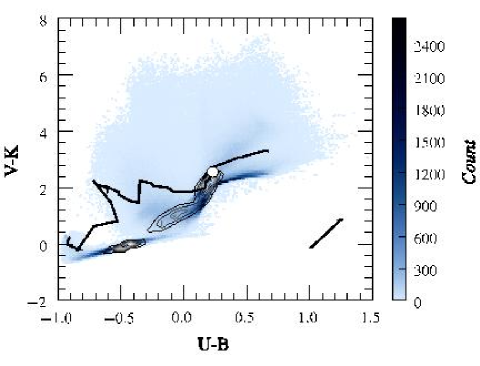
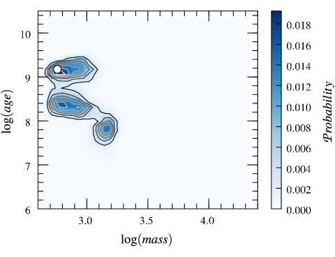
Figure 14: Example of probability maps for a population of $2.3$ Gyr and $780$ M_⊙ based on UBVIK band. Symbols and contours are the same as on Fig. 13. Age and mass estimates have been computed over 40 bins (refer to the binning issue described in Sect. 6.2 and also related to Fig. 15).

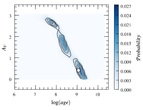
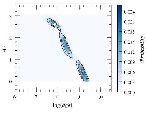
Figure 15: Illustration of the effect of binning using the cluster of Fig. 14. On left-hand side panel the correct age is recovered with 40 bins, however as the right panel illustrates, a different binning (50 bins) favours a much younger age with (erroneously) high extinction. The cluster is now moved to feature 5$.b$ in Fig.5.