Flux emergence and coronal eruption

Abstract

Aims. Our aim is to study the photospheric flux distribution of a twisted flux tube that emerges from the solar interior. We also report on the eruption of a new flux rope when the emerging tube rises into a pre-existing magnetic field in the corona.

Methods. To study the evolution, we use 3D numerical simulations by solving the time-dependent and resistive MHD equations. We qualitatively compare our numerical results with MDI magnetograms of emerging flux at the solar surface.

Results. We find that the photospheric magnetic flux distribution consists of two regions of opposite polarities and elongated magnetic tails on the two sides of the polarity inversion line (PIL), depending on the azimuthal nature of the emerging field lines and the initial field strength of the rising tube. Their shape is progressively deformed due to plasma motions towards the PIL. Our results are in qualitative agreement with observational studies of magnetic flux emergence in active regions (ARs). Moreover, if the initial twist of the emerging tube is small, the photospheric magnetic field develops an undulating shape and does not possess tails. In all cases, we find that a new flux rope is formed above the original axis of the emerging tube that may erupt into the corona, depending on the strength of the ambient field.

1 Introduction

Active regions are often associated with episodes of magnetic flux emergence from the solar interior (Zwaan (1985) and references therein). An important question then is, what is the evolution of the magnetic field configuration at the photosphere during emergence? Observations of emerging flux regions (EFRs) as recorded at the photospheric level, show that they consist of two main flux bundles of opposite magnetic polarity that may be the manifestation of an emerging flux tube. There is strong evidence that, in many EFRs, the rising magnetic fields are twisted. The idea of a flux rope configuration has been supported by photospheric measurements and observations of emerging fields in normal and complex (the so-called $\delta$ sunspot) ARs (Tanaka, 1991; Lites et al., 1995; Leka et al., 1996; Canou et al., 2009).

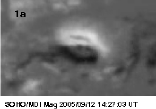
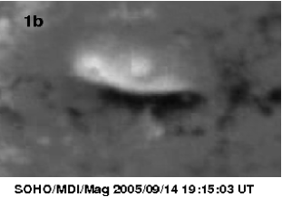
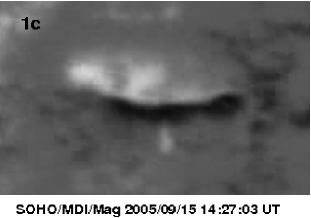
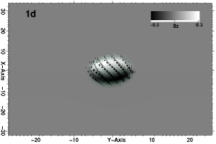
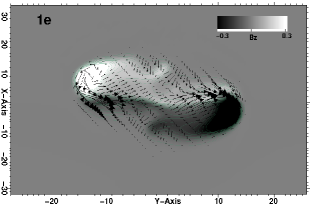
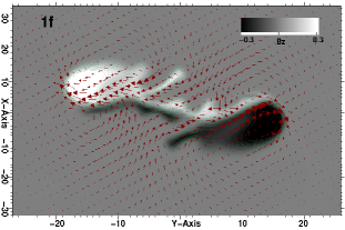
Figure 1: Top: SOHO/MDI magnetograms during flux emergence in NOAA AR 10808. Bottom: Magnetograms produced in the numerical experiments, at $z=21$ and $t=40$, $t=125$ and $t=175$ for the panels 1d-1f respectively. Arrows show the horizontal component of the magnetic field, $B_{hor}$ (panels 1d and 1e, black) and velocity field, $V_{hor}$ (panel 1f, red).

A common feature in EFRs is the presence of magnetic tongues or tails, which are connected with the main polarities on the two sides of the PIL of the AR (Li et al., 2007; Canou et al., 2009; Chandra et al., 2009). The appearance of magnetic tails is interpreted as the result of the emergence of twisted magnetic field lines at the photosphere (López Fuentes et al., 2000). However, a study of how the formation and evolution of the tails depend on the physical properties of the emerging field is still missing. Canou et al. (2009) used SOHO/MDI magnetograms and they reported on the existence of tails, which formed along the PIL and accompanied the emergence of magnetic flux in the region NOAA AR 1808. The shape of the tails was deformed during the evolution of the system. They also used the THEMIS vector magnetogram to reconstruct the coronal field (via a nonlinear force-free model) and found evidence for a pre-eruptive twisted flux tube above the emerging field.
In this paper, for the first time, we focus on the photospheric distribution of an emerging flux tube and the formation of the tails, showing the relationship between the topology of the tails and the initial tube parameters. We compare some of the numerical results with the observations by Canou et al. (2009) and we find a preliminary, qualitative agreement. Secondly, we report on the emergence of the tube into a magnetized corona and the subsequent coronal eruption of a flux rope. Similar to previous experiments (Magara, 2001; Manchester et al., 2004; Archontis & Hood, 2008; Archontis & Török, 2008; Hood et al., 2009), we find that the emerging twisted flux tube and the coronal rope are two distinct structures. More importantly, we find that the evolution of the erupting rope (ejective vs confined eruption) depends on the strength of the ambient field.

2 Model

The results in our experiments are obtained from a 3D MHD simulation. The basic setup of the experiment follows the simulation by Archontis et al. (2005) and consists of a hydrostatic atmosphere and a horizontal twisted magnetic flux tube. All variables are made dimensionless by choosing photospheric values of density, $\rho_{\mathrm{ph}}=3\times 10^{-7}\,\mathrm{g}\,\mathrm{cm}^{-3}$, pressure, $p_{\mathrm{ph}}=1.4\times 10^{5}\,\mathrm{ergs}\,\mathrm{cm}^{-3}$, and pressure scale height, $H_{\mathrm{ph}}=170\,\mathrm{km}$, and by derived units (e.g., magnetic field strength $B_{\mathrm{ph}}=1300\,\mathrm{G}$, velocity $V_{\mathrm{ph}}=6.8\,\mathrm{km}\,\mathrm{s}^{-1}$ and time $t_{\mathrm{ph}}=25\,\mathrm{s}$). The atmosphere includes a subsurface layer $(-10\leq z<20)$, photosphere $(20\leq z<30)$, transition region $(30\leq z<40)$, and corona $(40\leq z\leq 110)$. The numerical domain has a dimensionless size of $[-70,70]\times[-80,80]\times[-10,110]$ in the longitudinal ($x$), transverse ($y$) and vertical ($z$) directions, respectively. The magnetic flux tube is imposed $1.4Mm$ below the surface along the $y$-axis. The radius of the tube is $425Km$. The axial field is defined by $B_{y}=B_{0}\,\mathrm{exp}(-r^{2}/R^{2})$ and $B_{\phi}=\alpha\,r\,B_{y}$, where $r$ is the radial distance from the tube axis and $\alpha$ is the twist per unit length. The twist of the fieldlines around the axis of the tube is uniform. The tube is made buoyant by applying a density perturbation $\Delta\,\rho=[p_{t}(r)/p(z)]\,\rho(z)\,\mathrm{exp}\,(-y^{2}/\lambda^{2})$, where $p_{t}$ is the pressure within the flux tube and $\lambda$ is the buoyant part of the tube. We perform four experiments: E1 ($B=3,\alpha=0.4,\lambda=10$), E2 ($B=5,\alpha=0.4,\lambda=10$), E3 ($B=5,\alpha=0.4,\lambda=20$) and E4 ($B=5,\alpha=0.1,\lambda=10$). In the numerical domain, we use periodic boundary conditions in horizontal directions and closed boundaries with a wave damping layer in vertical directions.

3 Results

3.1 Emergence into the photosphere

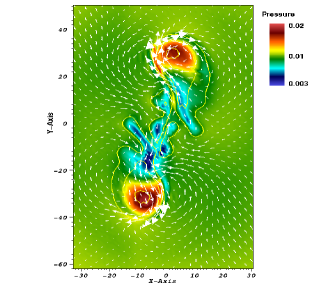
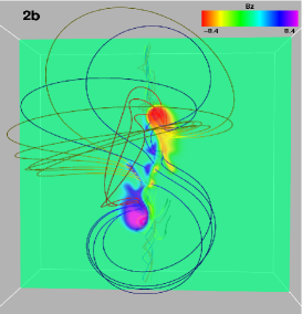
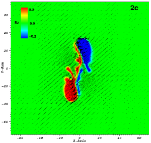
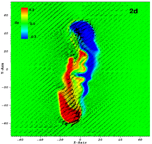
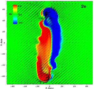
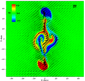
Figure 2: Top: The colour-scaled maps correspond to the $P_{tot}$ (2a) and $B_{z}$ (2b, 2c). Contours show $B_{z}$ and arrows the horizontal velocity. Time is $t=165$ and $z=25$, all for experiment E1. Bottom: Distribution of $B_{z}$ for E2 (2d), E3 (2e) and E4 (2f).

Figure 1 (panels 1a-1c) shows the evolution of the emerging field in the NOAA AR 10808. At the beginning (panel 1a) there is a clear appearance of a bipolar region at the photosphere with a North-South orientation. The two polarities progressively diverge from each other in an approximate East-West direction (panels 1b, 1c). During the evolution of the system, two elongated tails or tongues are formed in the wake of the two polarities (panel 1b). Initially, the tails possess an apparently coherent shape but as time goes on their structure appears to be more fragmented on the two sides of the PIL (panel 1c).

Panels 1d-1f show the photospheric distribution of the emerging field in our numerical experiments. Panel 1d shows the bipolar appearance of the emerging field, shortly after it intersects the photosphere. The North-South orientation of the bipolar field is due to the strong initial twist of the flux tube. Eventually (panel 1e), the two main polarities drift apart toward an East-West orientation. Similar to the observations, they are followed by magnetic tails that develop an intricate geometrical shape. The projection of the horizontal component of the magnetic field (arrows) is overplotted onto the magnetograms of panels 1d and 1e. At $t=40$, the direction of the horizontal magnetic field vectors shows a normal configuration, i.e. from the positive to the negative polarity, at the PIL. Later on, as more magnetic flux emerges from the solar interior, the direction of the magnetic field reveals a dominant inverse configuration along the PIL. This is due to the rise of the original axis of the twisted flux tube above this height ($z=21$). However, the main axis does not emerge above $2-3$ pressure scale heights, as has been shown in previous experiments of flux emergence (Fan, 2001; Magara, 2001; Archontis et al., 2005).

At a later stage of the evolution (Panel 1f), the elongated tails develop fingers seperated by dips along the curved PIL. In the fingers, the magnetic field remains strong (around $70\%$ of the maximum value of $B_{z}$ at this height). At the dips, the magnetic field is weak and the plasma density is relatively small. In fact, we find that there is a good correlation between the location of the dips and sites where plasma is moving in the transverse direction. There, the converging flows may reach values up to $3Km/s$ and the kinetic energy density becomes larger than the magnetic energy of the field. Thus, it seems that the shape of the magnetic tails is deformed due to inflows that are able to compress and advect the magnetic field. The origin of the inflows depends on the evolution of the total pressure ($P_{tot}$ = magnetic + gas pressure) at photospheric heights. Panel 2a shows the distribution of $P_{tot}$ at $z=25$, when the outer magnetic field has expanded into the corona. Due to the rapid expansion, a total pressure deficit has developed at the central area of the EFR and so the plasma moves towards the small pressure, and deforms the tails.

The link between the appearance of the tails and the topology of the fieldlines is shown in panel 2b. The yellow fieldlines have been traced from a far edge of the fingers (at $x=-11$, $y=0$). These are the outermost fieldlines with a strongly azimuthal nature. The blue fieldlines are highly twisted and are traced from the fingers of the tails that are closer to the PIL. They make a full turn around the main axis of the emerging tube connecting the central area of the two tails. The red fieldlines have been traced from the region closer to the main positive polarity of the field. They are very weakly twisted, possessing an arch-like bundle of fieldlines, joining the two sunspots. These fieldlines do not go through the tails. The above configuration shows that the appearance of the tails is due to the projection of the azimuthal component of the magnetic field at the photosphere.

Panels 2c-2f show the magnetic flux distribution at the photosphere for the experiments E1-E4 respectively. We take as a reference case the E1 and we examine the effect of varying the initial field strength ${\bf B}$, $\lambda$ and $\alpha$ on the appearance of the tails. For comparison, we consider the configuration of the field at a certain time for all experiments. The increase of ${\bf B}$ (in E2) results in keeping a coherent shape of the tails for a longer time period: at $t=165$, the tails in E2 are less fragmented than in E1. This is due to the fact that the total pressure within the EFR is large enough for the tails to be distinctively deformed by the inflows. However, we should emphasize that the shape of the tails is altered at a later time, when the two sunspots have seperated enough and the magnetic field in the EFR becomes weak. The increase of ${\lambda}$ (panel 2e) affects the downward tension of the fieldlines upon the buoyant part of the emerging field. The tension is less in the E3 and the field is emerging at the photosphere relatively faster. Thus, at a certain time, the magnetic field at the photosphere appears stronger in E3 than in E2. As we mentioned above, the stronger the magnetic field the less effective is the deformation of the tails’ shape. This is clearly shown in panel 2e, compared to the E2 (panel 2d). Also, the appearance of the tails critically depends on the initial twist of the emerging field. In E4, the twist parameter $\alpha$ is equal to 0.1 and the emerging field is almost horizontal and parallel to the E-W direction, shortly after its arrival to the photosphere. We find that there is no tail formation when the emerging field has $\alpha<0.2$. In this case, the EFR consists of the two sunspots and patches of magnetic flux with mixed polarity on the two sides of the PIL. Some of these photospheric flux segments are connected with the same fieldlines, possessing an overall undulating magnetic system. This is reminiscent of the “sea-serpent” configuration, which is produced during the emergence of a magnetic flux sheet. The latter develops undulations when it becomes unstable to the Parker instability (Archontis & Hood, 2009).

3.2 Eruption into the corona

In Section 3.1, we showed that the photospheric fingerprints of the EFR in E1 consist of features (e.g. tails) with a similar configuration to observed ARs (e.g. the AR 10808). In addition, the activity in the region NOAA AR 10808 is known to lead to filament and CME eruption (Canou et al., 2009). Thus, an important question is whether our twisted flux tube model can produce a coronal eruption. Our experiment shows that a new flux rope is formed above the original axis of the emerging flux tube due to reconnection of sheared fieldlines. The reconnection occurs in the higher photosphere/lower chromosphere in a similar manner to the model by van Ballegooijen & Martens (1989). A key issue is whether this eruption is confined (and, thus, the flux rope cannot fully escape into the outer atmosphere) or ejective. In previous experiments, Archontis & Török (2008) found that the inclusion of a pre-existing magnetic field in the corona may induce a runaway situation, via reconnection, during which the new flux rope fully erupts into the outer solar atmosphere. Here, we perform a similar experiment but using different initial parameters for the pre-existing coronal field. Our aim is to study whether the field strength of the ambient field affects the rising motion of the erupting flux rope.

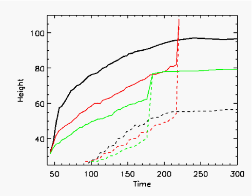
Figure 3: Height-time profiles of the apex of the emerging field (solid) and the flux rope (dashed) in experiments B1 (black), B2 (red) and B3 (green).

The observed magnetogram in the AR 10808 shows that the emerging flux is rising into a pre-existing field oriented in the E-W direction. The emerging field has a N-S orientation and, thus, the relative orientation of the two fields is about 90 degrees. To simulate this, we include a horizontal and uniform magnetic field in the corona along the y-axis, parallel to the main axis of the twisted tube (for example, see Archontis et al. (2005)). To a first approximation, this field may correspond to the upper part of the observed AR’s field, which is likely to be anchored in the surrounded diffuse polarities. We find that the field strength of the ambient field ($B_{amb}$) plays a critical role in the eruptive motion of the new flux rope. Figure 3 shows the height-time profile of the front of the emerging field (solid lines) and the center of the new flux rope (dashed lines) for three experiments (B1, B2 and B3) where: $B_{amb}=0.003$ (B1, black lines) , $B_{amb}=0.015$ (B2, red lines) and $B_{amb}=0.03$ (B3, green lines) respectively. The heights are calculated at the vertical midplane after the emerging field enters the transition region.

In B1, the front of the expanding tube rises slowly within the magnetized corona and eventually it saturates at a height of $z\approx 96$. The new flux rope is formed at the low atmosphere at $t\approx 95$ and, thereafter, it follows a similar evolution to the envelope field of the expanding tube. Firstly, it rises almost linearly with time but then it reaches an equilibrium where the magnetic pressure force is balanced by the tension of the fieldlines. In this case, the eruption is confined: the flux rope is trapped within the envelope field. In B2, the apex of the emerging field reaches lower heights during its rising motion. This is because it comes into contact with an ambient field that is stronger and able to delay the emergence. At the same time, a considerable amount of the rising magnetic flux is removed from the envelope field due to reconnection. As a result, the distance between the new flux rope and the front of the envelope field is reduced. As more magnetic layers above the flux rope are peeled off, the downward tension of the envelope fieldlines decreases. Eventually, the flux rope experiences an ejective eruption reaching the upper boundary of the domain very quickly. Due to the short distance between the erupting rope and the closed top boundary, the velocity of the center of the flux rope is restricted to $197Km/s$. However, the plasma underneath the flux rope is rising with even higher velocity at $\approx 350Km/sec$. This is a reconnection jet that is formed due to internal (i.e. within the EFR) reconnection of fieldlines and helps the flux rope to accelerate during its eruption. According to these calculations, it is possible that the rise of the flux rope might account for a CME-like eruption.

In B3, the eruption of the flux rope is triggered earlier. Again, this is because the stronger ambient field reconnects more effectively with the flux above the rope and removes more magnetic layers from the emerging system. However, for the same reason, the front of the envelope field rises with a slower rate and the distance between the new flux rope and the front decreases. As a result, soon after the triggering of the ejective eruption, the erupting rope collides with the front and loses its distinct circular shape, possibly due to reconnection with the ambient field. After the collision, the leading edge of the emerging system is lifted up for a few pressure scale heights. However, it does not reconnect effectively with the magnetic flux above it, and eventually reaches a quasi-static state at a height of $z\approx 80$. Thus, in B3, the ejective flux rope is trapped by the dominant ambient field and not by the envelope field.

4 Summary and Discussion

In this paper, we have presented a 3D model to study the emergence of a twisted flux tube throughout the solar atmosphere. Our model gives new insights into the photospheric distribution of the emerging magnetic field: it consists of a bipolar region and tails on the two sides of the PIL. The appearance of tails reveal that the emerging magnetic field is twisted. For small twist, the emerging field possess undulations. Our results predict that the irregular structure of the tails is due to the interplay between the flows and the dynamical evolution of the magnetic field. The configuration of the emerging field at the photosphere is in qualitative agreement with observations (Canou et al., 2009).

In agreement with previous simulations, our experiments show the eruption of a flux rope, which is formed above the original axis of the emerging tube. For the first time, we find that the field strength of a pre-existing coronal magnetic field is a crucial parameter affecting the eruptive phase of the rope. Under the specific conditions of the present experiments, we found that the eruption is ejective when $0.01<B_{amb}<0.02$. For other values, the eruption is confined within the envelope field.

The aim of these experiments is not a direct comparison with the observations, but rather to suggest possible mechanisms that drive the dynamical behaviour of the system. Further experiments are required to verify the effect of the initial parameters (e.g. field strength, radius, initial atmospheric height and twist, etc.) of the twisted flux tube and the pre-existing field on (a) the characteristics of its photospheric appearance (formation and evolution of the tails, shear and transverse flows, etc.) and (b) the dynamics of the associated eruption.