$U(1)$ slave-particle study of the finite-temperature doped Hubbard model in one and two dimensions

Abstract

One-dimensional systems have unusual properties such as fractionalization of degrees of freedom. Possible extensions to higher dimensional systems have been considered in the literature. In this work we construct a mean field theory of the Hubbard model taking into account a separation of the degrees of freedom inspired by the one-dimensional case and study the finite-temperature phase diagram for the Hubbard chain and square lattice. The mean field variables are defined along the links of the underlying lattice. We obtain the spectral function and identify the regions of higher spectral weight with the fractionalized fermionic (spin) and bosonic (charge) excitations.

I introduction

The Hubbard model is one of the simplest models accounting for interactions between electrons and has been used to describe various strongly correlated materials. It is parameterized by only two constants, a kinetic term scaled in the tight-binding approximation by the hopping amplitude $t$ and an on-site interaction $U$ modeling the Coulomb repulsion felt by two electrons of opposite spins occupying the same site.

The exact solution of the one-dimensional Hubbard model by the Bethe ansatz Lieb and Wu (1968) involves composite degrees of freedom that correspond to different rapidity branches. In addition to a $c0$ charge-momentum rapidity, there are sets of $(\alpha,\nu)$ rapidities Takahashi (1972). The general rapidity branch label $\alpha\nu$ is such that $\alpha=c,s$ and $\nu=0,1,2,...$ for $\alpha=c$ and $\nu=1,2,...$ for $\alpha=s$. The $(c,\nu)$ and $(s,\nu)$ rapidities are associated with the charge and spin degrees of freedom, respectively. For electronic densities $n\leq 1$, the ground state has finite occupancies for the charge $(c,0)$ and spin $(s,1)$ branches only. The relation between the original electrons and the entities that describe the eigenstates of the Hubbard model is however complex and only recently some light has emerged Carmelo et al. (2004a).

Electron double occupancy is a good quantum number (it is conserved) in the limit of $U\rightarrow\infty$ but for finite values of $U/t$ it is not conserved. However, it is possible to define new fermionic operators, associated with fermionic objects called rotated electrons, through a canonical transformation, $\hat{V}$, such that the double occupancy of these rotated electrons is a good quantum number for all finite values of $U/t$ Harris and Lange (1967); Carmelo et al. (2004a); Stein (1997); MacDonald et al. (1988). In terms of the rotated electrons, it is a consistent interpretation of the Bethe ansatz states to describe the various branches (rapidities) in terms of, first, a separation into empty, double-occupied and singly occupied sites. The empty and double-occupied sites are called $\eta$-spin $1/2$ holons Carmelo et al. (2004a) and the singly-occupied give rise to a charge part that originates the $(c,0)$ particles and to a spin part which originates the spin-$1/2$ spinons. The $\eta$-spin projection $1/2$ (and $-1/2$) holons correspond to rotated-electron unoccupied sites (and doubly-occupied sites). The spinons of spin projection $\pm 1/2$ refer to the spins of the rotated electrons which singly occupied sites. Second, these are paired in singlets ($s,1$) or in pairs of pairs of singlets and so on ($s,\nu$). The holons are also paired in such a way that empty sites and doubly-occupied sites are paired ($c,\nu$). These results apply to the rotated electrons and not to the original electrons. They are however related by the above mentioned canonical transformation. At high values of $U$ they are very close and identical when $U\rightarrow\infty$. For many practical situations, such as the calculation of various correlation functions, it is a reasonably good approximation to consider the rotated electrons as similar to the original electrons Carmelo et al. (2000); Sing et al. (2003); Carmelo et al. (2004b); Carmelo and Penc (2006); Bozi et al. (2008).

There are transformations in the literature that propose a similar decoupling of the electronic degrees of freedom. This can be seen for instance in Kotliar and Ruckenstein (1986) or in Zou and Anderson (1988). The main motivation was the study of either the large-$U$ limit in the Hubbard or Anderson models Dorin and Schlottmann (1992) with the intent to control in an efficient way the projection to states where double occupancy is restricted (as in the $t-J$ model) but considering a finite value of $U$ instead of the extreme case of infinite $U$, usually taken care of by a single slave boson Coleman (1984). In the Zou-Anderson transformation (ZA) each physical electron is mapped into the one particle sector of a set of four particles, two fermions and two bosons. The two bosons may be chosen as spinless particles and represent the empty and doubly occupied states of each lattice site; excitations of these two degrees of freedom are called holons and doublons and can be interpreted as carrying no charge or $-2e$ respectively. The fermions then represent singly occupied states with spin $\pm 1/2$, excitations on this sector are called spinons and carry charge $-e$. However, the charges may be defined differently, as considered in the original paper by Zou and Anderson Zou and Anderson (1988). There is also an exact transformation that explicitly includes spin and charge separation Östlund and Granath (2006) introducing two sets of operators as quasicharge (fermionic) and quasispin (spin-like). The representation of the quasispin operators leads however in general to bilinear terms in bosons or fermions and therefore this leads to six operator terms in the Hamiltonian.

The ZA mapping reverses the role of the interacting and kinetic terms in the Hamiltonian. The interacting Hubbard term becomes quadratic in the ZA particles and the kinetic one is transformed into an interacting quartic term that couples particles along the lattice links.  This is particularly useful to study the strong interacting (large U) regime where the kinetic term is treated as a perturbation. The price of this transformation is the appearance of an on-site constraint which assures exactly one particle per lattice site. In the mean field (MF) approach this translates to an on-site Lagrange multiplier. Generically slave-particle methods induce new unphysical symmetries of the Hamiltonian written in terms of slave particles, that are called in this context gauge symmetries. In this particular case the symmetry group is U(1).

We note that the representation introduced by Zou and Anderson has been used to explicitly obtain an exact solution of the Hubbard chain in the large $U$ limit in a much simpler way as compared to the Bethe ansatz Dias and dos Santos (1992). Also it has been used to study the stiffness of the one-dimensional Hubbard model in a way equivalent and complementar to the Bethe ansatz solution Peres et al. (2000).

In the large U limit it is very costly to create doubly occupied sites. It is usual to consider $d=0$ Lee et al. (2006) (projection to subspace of no-double occupancy) or to perform a canonical transformation to eliminate transitions to doubly occupied sites Zou and Anderson (1988). This type of procedure leads to a treatment similar to the $t-J$ model, appropriate near half filling in the vicinity of magnetic order for a square lattice.

It has been argued recently that one should instead integrate out the high-energy scale to obtain an effective low-energy theory which has been shown to contain a charge $2e$ bosonic mode Leigh et al. (2007); Choy et al. (2008); Phillips et al. (2009). This mode may be bound to a hole, providing a possible explanation of the pseudogap observed in high-$T_{c}$ materials. In this work we will maintain the full structure of the transformation between the electron operators and the auxiliary particles introduced in the Zou-Anderson transformation. We will be focusing on the finite energy (finite temperature) properties where we will find and study phases with non-standard correlation functions associated with the fractionalized degrees of freedom. We will obtain the phase diagrams for one- and two-dimensional systems and calculate various correlation functions as well as the spectral function.

We will use nonlocal decouplings of the auxiliary operators leading to link variables that can be associated with nearest-neighbor spin singlets or bound-states between empty and doubly occupied sites in a way close to the Bethe ansatz solution and also suggested by the treatment of Ref. Phillips et al. (2009), imposing at MF level the existence of these states. A simplified treatment of link variables was introduced in Ref. Vicente Alvarez et al. (1995) and the significance of short-range correlations between empty and doubly occupied sites was, for instance, determined in Ref. Kaplan et al. (1982). We note that bond variables appear naturally in extensions of the Hubbard model too, for instance nearest-neighbor interactions, or bond correlated hoppings Japaridze and Kampf (1999). Interestingly, many results have been obtained for systems where the hopping between singly occupied sites and empty and doubly occupied sites is eliminated, implying that double occupancy is a good quantum number Strack and Vollhardt (1993); Arrachea and Aligia (1994); Dolcini and Montorsi (2002).

The paper is organized as follows: in section II we discuss the methods used to construct the MF solution. In section III we discuss the MF phase diagram for the Hubbard chain and the square lattice and in section IV we discuss the spectral function for both cases, interpreted in terms of the fractional excitations here considered. Finally in section V we discuss the results obtained and in the appendix we present a list of MF solutions for the square lattice.

II methods

We start from the $U(1)$ representation of the Hubbard model introduced by Zou and Anderson (ZA) Zou and Anderson (1988), $c_{r,\sigma}^{\dagger}=e_{r}\,s_{r,\sigma}^{\dagger}+\sigma d_{r}^{\dagger}\,s_{r,-\sigma}$ which maps a spin-$1/2$ fermion (the physical electron) to the one-particle subspace of four fields $e_{r},d_{r},s_{r,\sigma=\pm 1}$. In this work bosonic $e_{r}$ and $d_{r}$ fields (where $r$ labels the lattice sites) are considered corresponding to the annihilation of empty and doubly occupied sites, $s_{r,\sigma=\pm 1}$ are fermions that carry the spin degree of freedom. The opposite choice of statistics ($e,d$ fermions and $s_{\pm 1}$ bosons) is also possible leaving the mapping unchanged. The Hamiltonian of the Hubbard model is given by

$$H-\mu\,n_{T} = -t\sum_{r,\delta>0,\sigma}c_{r,\sigma}^{\dagger}c_{r+\delta,\sigma}+c_{r+\delta,\sigma}^{\dagger}c_{r,\sigma}+U\sum_{r}n_{r,1}n_{r,-1}-\mu\sum_{r,\sigma}n_{r,\sigma},$$ (2)

$$= t\sum_{r,\delta>0}\left[\left(d_{r}^{\dagger}d_{r+\delta}-e_{r}^{\dagger}e_{r+\delta}\right)^{\dagger}\left(s_{r,1}^{\dagger}s_{r+\delta,1}+s_{r-1}^{\dagger}s_{r+\delta,-1}\right)+\left(s_{r,1}^{\dagger}s_{r+\delta,1}+s_{r-1}^{\dagger}s_{r+\delta,-1}\right)^{\dagger}\left(d_{r}^{\dagger}d_{r+\delta}-e_{r}^{\dagger}e_{r+\delta}\right)\right.$$

$$\left.+\left(d_{r}e_{r+\delta}+e_{r}d_{r+\delta}\right)^{\dagger}\left(s_{r,1}s_{r+\delta,-1}-s_{r,-1}s_{r+\delta,1}\right)+\left(s_{r,1}s_{r+\delta,-1}-s_{r,-1}s_{r+\delta,1}\right)^{\dagger}\left(d_{r}e_{r+\delta}+e_{r}d_{r+\delta}\right)\right]$$

$$+U\sum_{r}d_{r}^{\dagger}d_{r}-\mu\sum_{r}(1+d_{r}^{\dagger}d_{r}-e_{r}^{\dagger}e_{r})$$

where $\delta$ is a directed lattice vector connecting nearest neighbor sites, $\mu$ is the chemical potential and $n_{T}$ the total number of electrons.

Using the ZA mapping the partition function is given in a path integral formulation by

$$Z = \int D\lambda DeDdDs_{\sigma}\ e^{-\int_{0}^{\beta}\ d\tau\,L}$$ (3)

$$L = \sum_{r}d_{r}^{\dagger}(\partial_{\tau}+\lambda_{r}+U-\mu)d_{r}+$$ (4)

$$\sum_{r}e_{r}^{\dagger}(\partial_{\tau}+\lambda_{r}+\mu)e_{r}+\sum_{r}s_{r,\sigma}^{\dagger}(\partial_{\tau}+\lambda_{r})s_{r,\sigma}$$

$$+\sum_{r,\delta}t_{\delta}\,tr\left[\mathbf{B}_{r,r+\delta}.\mathbf{F}_{r,r+\delta}\right]-\sum_{r}\lambda_{r}-\mu V$$

where

$$\mathbf{B}_{i,j} = \left(\begin{array}[]{c|c}\mathit{d}_{j}^{\dagger}\text{ }\mathit{d}_{i}-\mathit{e}_{j}^{\dagger}\mathit{e}_{i}&\mathit{d}_{i}^{\dagger}\mathit{e}_{j}^{\dagger}+\mathit{d}_{j}^{\dagger}\mathit{e}_{i}^{\dagger}\\ \hline\cr\mathit{e}_{i}\mathit{d}_{j}+\mathit{e}_{j}\mathit{d}_{i}&\mathit{d}_{i}^{\dagger}\mathit{d}_{j}-\mathit{e}_{i}^{\dagger}\mathit{e}_{j}\end{array}\right);$$ (7)

$$\mathbf{F}_{i,j} = \left(\begin{array}[]{c|c}\mathit{s}_{i,-1}^{\dagger}\mathit{s}_{j,-1}+\mathit{s}_{i,1}^{\dagger}\mathit{s}_{j,1}&\mathit{s}_{i,-1}^{\dagger}\mathit{s}_{j,1}^{\dagger}-\mathit{s}_{i,1}^{\dagger}\mathit{s}_{j,-1}^{\dagger}\\ \hline\cr\mathit{s}_{j,1}\mathit{s}_{i,-1}-\mathit{s}_{j,-1}\mathit{s}_{i,1}&\mathit{s}_{j,-1}^{\dagger}\mathit{s}_{i,-1}+\mathit{s}_{j,1}^{\dagger}\mathit{s}_{i,1}\end{array}\right);$$ (10)

are respectively bosonic and fermionic matrices, $\lambda_{r}$ is an on-site real field inserted in order to project to the one-particle sector $n_{r}^{\text{ZA}}=d_{r}^{\dagger}d_{r}+e_{r}^{\dagger}e_{r}+\sum_{\sigma}s_{r,\sigma}^{\dagger}s_{r,\sigma}=1$ with$\int D\lambda=\int_{0-i\,\pi/\beta}^{0+i\,\pi/\beta}\prod_{r}\prod_{\tau}i\frac{d\lambda_{r}(\tau)}{2\pi\beta^{-1}}$, and $V$ is the total number of lattice sites. Using the identity: $\int d\mu\left(\boldsymbol{Q}^{\dagger},\boldsymbol{Q}\right)e^{-\text{Tr}\left[\boldsymbol{Q}^{\dagger}.\boldsymbol{Q}+\boldsymbol{C}^{\dagger}.\boldsymbol{Q}+\boldsymbol{Q}^{\dagger}.\boldsymbol{A}\right]}=e^{\text{Tr}\left[\boldsymbol{C}^{\dagger}.\boldsymbol{A}\right]},$ with $d\mu\left(\boldsymbol{Q}^{\dagger},\boldsymbol{Q}\right)=\prod_{i,j}\frac{d\bar{Q}_{j,i}dQ_{i,j}}{2\pi i}$ and $\left[\boldsymbol{Q}^{\dagger}\right]_{i,j}=\bar{Q}_{i,j}$, $\left[\boldsymbol{Q}\right]_{i,j}=Q_{i,j}$($\bar{Q}_{j,i}=Q_{i,j}^{*}$), we introduce a $2\times 2$ matricial Hubbard-Stratonovich (HS) field in order to decouple the fermionic and bosonic terms:

$$Z = \int D\lambda DeDdDs_{\sigma}D\boldsymbol{Q}\ e^{-\int_{0}^{\beta}\ d\tau\,L}$$ (12)

$$L = \sum_{r}d_{r}^{\dagger}(\partial_{\tau}+\lambda_{r}+U-\mu)d_{r}+\sum_{r}e_{r}^{\dagger}(\partial_{\tau}+\lambda_{r}+\mu)e_{r}$$ (13)

$$+\sum_{r}s_{r,\sigma}^{\dagger}(\partial_{\tau}+\lambda_{r})s_{r,\sigma}-\sum_{r}\lambda_{r}$$

$$-\mu V+\sum_{r,\delta}\text{Tr}\left[\boldsymbol{Q}_{r,\delta}^{\dagger}.\boldsymbol{Q}_{r,\delta}\right]$$

$$+\sum_{r,\delta}\sqrt{t_{\delta}}\text{Tr}\left[\boldsymbol{Q}_{r,\delta}^{\dagger}.\mathbf{F}_{r,r+\delta}-\mathbf{B}_{r,r+\delta}.\boldsymbol{Q}_{r,\delta}\right].$$

The additional gauge freedom introduced when writing the Hubbard model in this particular slave-particle form is $U(1)$ and is implemented by the operator $U(\phi)=\prod_{r}e^{-i\phi_{r}n_{T,r}}$. Such gauge transformation changes the ZA particle fields by a site dependent phase $a_{r}\to e^{-i\phi_{r}}a_{r}$ ($a=s_{\pm},d,e$) which gives the simple transformation rule for the matrices $\mathbf{B}_{r,r+\delta}\to e^{-i\sigma_{z}\phi_{r+\delta}}.\mathbf{B}_{r,r+\delta}.e^{i\sigma_{z}\phi_{r}}$ and $\mathbf{F}_{r,r+\delta}\to e^{-i\sigma_{z}\phi_{r}}.\mathbf{F}_{r,r+\delta}.e^{i\sigma_{z}\phi_{r+\delta}}$. In order to leave the Lagrangian invariant, this transformation also induces a gauge transformation in the HS fields

$$\boldsymbol{Q}_{r,\delta} \to e^{-i\sigma_{z}\phi_{r}}.\mathbf{Q}_{r,\delta}.e^{i\sigma_{z}\phi_{r+\delta}},$$ (14)

defining also 6 on-site gauge invariant quantities: $\left[\boldsymbol{Q}_{r,\delta}\right]_{i,j}\left[\boldsymbol{Q}_{r,\delta}^{\dagger}\right]_{i,j}$ and $\left[\boldsymbol{Q}_{r,\delta}\right]_{i,j}\left[\boldsymbol{Q}_{r,\delta}\right]_{j,i}$($i,j$=1,2).

A MF treatment of this Lagrangian can be justified introducing $N$ copies of the ZA particles in order to perform a $1/N$ expansion that coincides with the usual MF approximation at zero order and organizes the following corrections in numbers of loopsLee et al. (2006). However, as in $SU(N)$ generalizations of spin-1/2 models, this parameter is rather unphysical and this approach will not be explicitly pursued here. The MF approximation is obtained varying the free energy with respect to the $\boldsymbol{Q}$ and $\lambda$ fields:

$$\boldsymbol{Q}_{r,\delta}(\tau) = -\sqrt{t_{\delta}}\left\langle\mathbf{F}_{r,\delta}(\tau)\right\rangle_{0}$$ (15)

$$\boldsymbol{Q}_{r,\delta}^{\dagger}(\tau) = \sqrt{t_{\delta}}\left\langle\mathbf{B}_{r,\delta}(\tau)\right\rangle_{0}$$ (16)

$$1 = \left\langle n^{ZA}(\tau))\right\rangle_{0},$$ (17)

where $\left\langle\ \right\rangle_{0}$ stands for the MF average. In order to study this set of equations a time and space translational invariant ansatz $\boldsymbol{Q}_{r,\delta}(\tau)=\boldsymbol{Q}_{\delta}$ was imposed. The saddle-point values of the HS fields describe hopping and pairing terms:

$$\chi_{F,r,\delta} = \left\langle\mathit{s}_{r+\delta,1}^{\dagger}\mathit{s}_{r,1}+\mathit{s}_{r+\delta,-1}^{\dagger}s_{r,-1}\right\rangle_{0},$$

$$\Delta_{F,r,\delta} = \left\langle\mathit{s}_{r+\delta,1}\mathit{s}_{r,-1}-\mathit{s}_{r+\delta,-1}\mathit{s}_{r,1}\right\rangle_{0},$$

$$\chi_{B,r,\delta} = \left\langle\mathit{d}_{r+\delta}^{\dagger}\mathit{d}_{r}-\mathit{e}_{r+\delta}^{\dagger}\mathit{e}_{r}\right\rangle_{0},$$

$$\Delta_{B,r,\delta} = \left\langle\mathit{d}_{r+\delta}\mathit{e}_{r}+\mathit{e}_{r+\delta}\mathit{d}_{r}\right\rangle_{0},$$ (18)

and Eqs. (15-16) are equivalent to

$$\boldsymbol{Q}_{r,\delta} = -\sqrt{t_{\delta}}\left(\begin{array}[]{cc}\chi_{F,r,\delta}^{\dagger}&\Delta_{F,r,\delta}^{\dagger}\\ \Delta_{F,r,\delta}&\chi_{F,r,\delta}\end{array}\right),$$ (21)

$$\boldsymbol{Q}_{r,\delta}^{\dagger} = \sqrt{t_{\delta}}\left(\begin{array}[]{cc}\chi_{B,r,\delta}&\Delta_{B,i,\delta}^{\dagger}\\ \Delta_{B,r,\delta}&\chi_{B,r,\delta}^{\dagger}\end{array}\right).$$ (24)

Note that the MF values obtained for $\boldsymbol{Q}^{\dagger}$ and $\boldsymbol{Q}$ are not complex conjugated of each other; this is crucial in order to interpret the zero order Lagrangian as coming from a hermitian MF Hamiltonian, in the extended Hilbert space, as noticed in Lee and Lee (2005); Vicente Alvarez et al. (1995). This corresponds to the analytic continuation of the $\boldsymbol{Q}$ fields and also occurs for $\lambda$. Care should be taken, however, when considering fluctuations of these fields around their MF values: as the $\lambda$ fluctuations are purely imaginary even if the MF value is real, the conjugated fluctuations of $\delta\chi_{F,r,\delta}$ are $\delta\chi_{B,r,\delta}^{\dagger}$ and not $\delta\chi_{F,r,\delta}^{\dagger}$ as the MF treatment could suggest. The filling fraction of the electrons is imposed as usual requiring the chemical potential to satisfy $x=1-\left\langle n_{T}\right\rangle=1-\frac{1}{V\beta}\partial_{\mu}\ln Z$, where $x$ is the hole doping.

Assuming translational invariance of the MF solutions, the MF Hamiltonian can be brought to a diagonal form in $k$ space. Defining $\tilde{\boldsymbol{b}}_{k}=\left\{d_{k},e_{-k,1},d_{k,1}^{\dagger},e_{-k,1}^{\dagger}\right\}^{T}$and $\tilde{\boldsymbol{s}}_{k}=\left\{s_{k,1},s_{-k,-1},s_{k,1}^{\dagger},s_{-k,-1}^{\dagger}\right\}^{T}$the Bogoliubov transformation diagonalizing the Lagrangian is given by

$$\boldsymbol{a}_{k} = R_{b}(k).\tilde{\boldsymbol{b}}_{k}$$

$$\boldsymbol{f}_{k} = R_{s}(k).\tilde{\boldsymbol{s}}_{k}$$ (25)

where $f_{\sigma=\pm}$ and $a_{i=e,d}$ are the fermionic and bosonic Bogoliubov transformed fields . In these new variables the Hamiltonian is given by

$$H = \sum_{k,i=d,e}\,a_{k,i}^{\dagger}\varepsilon_{i,k}a_{k,i}+\Theta_{B,k}$$ (26)

$$+\sum_{k,\sigma}\,f_{k,\sigma}^{\dagger}\varepsilon_{F,k}f_{k,\sigma}+\Theta_{F,k}$$

$$-V\lambda+V\sum_{\delta}\text{Tr}\left[\boldsymbol{Q}_{\delta}^{\dagger}.\boldsymbol{Q}_{\delta}\right]-V\left(\mu+\frac{U}{2}\right)$$

where the single particle energies $\varepsilon$ and the energy shifts $\Theta$ are given by

$$\varepsilon_{F,k} = \frac{1}{2}\left(\omega_{F,k}-\omega_{F,-k}+\sqrt{4\delta_{F,k}\bar{\delta}_{F,k}+\left(\omega_{F,-k}+\omega_{F,k}\right)^{2}}\right)$$

$$\Theta_{F,k} = -\frac{1}{2}\left[\varepsilon_{F,k}+\varepsilon_{F,-k}\right.$$

$$+\left.\chi_{B}(k)-\chi_{B}^{\dagger}(k)+\chi_{B}(-k)-\chi_{B}^{\dagger}(-k)\right]$$

$$\varepsilon_{d,k} = \frac{1}{2}\left(\omega_{d,k}-\omega_{e,-k}+\sqrt{\left(\omega_{e,-k}+\omega_{d,k}\right)^{2}-4\delta_{B,k}\bar{\delta}_{B,k}}\right)$$

$$\varepsilon_{e,k} = \frac{1}{2}\left(\omega_{e,k}-\omega_{d,-k}+\sqrt{\left(\omega_{e,k}+\omega_{d,-k}\right)^{2}-4\delta_{B,k}\bar{\delta}_{B,k}}\right)$$

$$\Theta_{B,k} = \frac{1}{2}\left[\varepsilon_{d,k}+\varepsilon_{e,-k}\right.$$ (27)

$$+\left.\chi_{F}(k)-\chi_{F}^{\dagger}(k)-\chi_{F}(-k)+\chi_{F}^{\dagger}(-k)\right]$$

with

$$\omega_{d,k} = U-\mu+\lambda+\chi_{F}(k)+\chi_{F}^{\dagger}(k)$$

$$\omega_{e,-k} = \mu+\lambda-\chi_{F}(-k)-\chi_{F}^{\dagger}(-k)$$

$$\delta_{B,k} = \Delta_{F}(-k)+\Delta_{F}(k)$$

$$\omega_{F,k} = \lambda+\chi_{B}(k)+\chi_{B}^{\dagger}(k)$$

$$\delta_{F,k} = \Delta_{B}(-k)+\Delta_{B}(k)$$ (28)

and $A(k)=\sum_{\delta=out}t_{\delta}e^{ik\delta}A_{\delta}$ ($A=\chi,\Delta$). Explicitly the Bogoliubov rotation matrices are given by

$$R_{s} = \left(\begin{array}[]{cccc}u_{F,k}&0&0&v_{F,k}\\ 0&u_{F,k}&-v_{F,k}&0\\ 0&\bar{v}_{F,k}&u_{F,k}&0\\ -\bar{v}_{F,k}&0&0&u_{F,k}\end{array}\right);$$ (33)

$$R_{b} = \left(\begin{array}[]{cccc}u_{B,k}&0&0&v_{B,k}\\ 0&u_{B,k}&v_{B,k}&0\\ 0&\bar{v}_{B,k}&u_{B,k}&0\\ \bar{v}_{B,k}&0&0&u_{B,k}\end{array}\right)$$ (38)

with

$$u_{F/B,k} = \frac{1}{\sqrt{1+\tau_{F/B}(k)\bar{\tau}_{F/B}(k)}}$$

$$v_{F/B,k} = \frac{\tau_{F/B}}{\sqrt{1+\tau_{F/B}(k)\bar{\tau}_{F/B}(k)}}$$

$$\tau_{F}(k) = \frac{\left(\omega_{F,k}+\omega_{F,-k}\right)-\sqrt{\left(\omega_{F,k}+\omega_{F,-k}\right)^{2}+4\delta_{F,k}\bar{\delta}_{F,k}}}{2\bar{\delta}_{F,k}}$$

$$\tau_{B}(k) = \frac{\left(\omega_{d,k}+\omega_{e,-k}\right)-\sqrt{\left(\omega_{d,k}+\omega_{e,-k}\right)^{2}-4\delta_{B,k}\bar{\delta}_{B,k}}}{2\bar{\delta}_{B,k}}$$

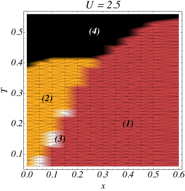
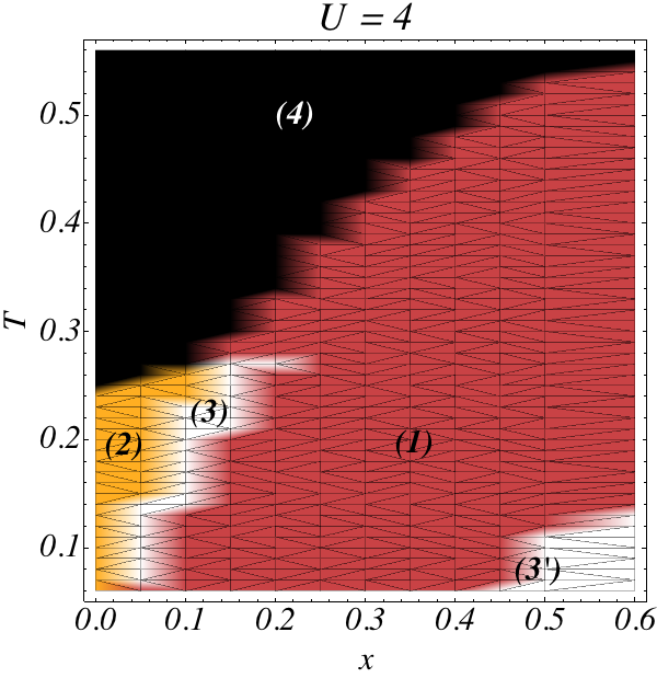
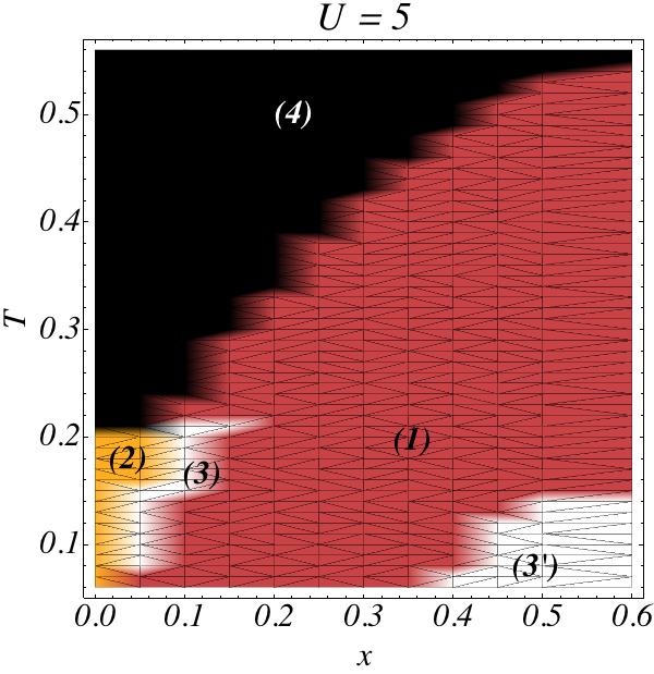
Figure 1: Mean Field phase diagram in the $x-T$ plane as a function of $U$ for a chain with $200$ sites. The colors represent the different types of solution minimizing the free energy: (1) $\chi\neq 0,\,\Delta=0$ (Red); (2) $\chi=0,\,\Delta\neq 0$ (Orange); (3) $\chi\neq 0,\,\Delta\neq 0$ (White); (4) $\chi,\Delta=0$ (Black). The calculated points are placed in the nodes of the finite mesh of the values of $x$ and $T$ considered, the colors plotted between nodes are interpolated.

The above treatment should be valid for arbitrary values of the interaction parameter $U$ once the double occupancy described by the $d$ bosonic field is fully taken into account. This should be of great importance near half-filling because in this regime $\left\langle d^{\dagger}d\right\rangle$ is not small compared to $\left\langle e^{\dagger}e\right\rangle$.

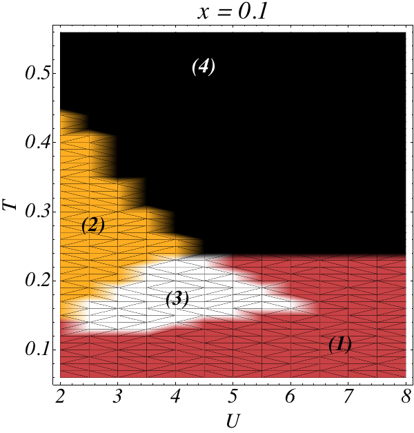
Figure 2: Mean Field phase diagram in the $U-T$ plane for $x=0.1$ for a chain with $200$ sites. The colors represent the different types of solution minimizing the free energy as in Fig. 1

Contrary to the $t-J$ model no canonical transformation was performed at this stage in the physical electrons. Note that discarding the $d$ field at this stage would yield diagonal $\mathbf{F}$ and $\mathbf{B}$ matrices and the subsequent MF decoupling would miss the phases of the ZA fermions with non-zero pairings $\Delta$. This kind of phases could however be considered if one adopts a variational procedure (Ref. Brinckmann and Lee (2001)). The $t-J$ model also presents an $\mathbf{S}\cdot\mathbf{S}$ term not present in Eq. (13) which is responsible for sub-lattice magnetization in the ground state of the square lattice Hubbard model near half-filing. Anti-ferromagnetic correlations will nevertheless be generated if one integrates out the $d$ fields before doing the MF decoupling; however, such procedure leads to six-body coupling terms and will not be considered here. Even if Eq. (13) can not produce sub-lattice magnetization we expect antiferromagnetic spin-spin correlation functions for non-frustrated lattices. In this work no boson condensation is considered away from $T=0$; this corresponds to a fully 1D or 2D model of holons $e$ and doublons $d$ Lee et al. (2006).

Eqs. (15-17) together with the fixed doping condition were solved numerically in one and two dimensions for several values of $U/t$ (typically in the range of 2 to 6) , for different values of doping $x\simeq 0,...,0.6$ and temperature. For the 2D case no particular symmetry based ansatz is implemented leading to some peculiar phases. Before discussing some of the MF solutions in detail a few remarks are in order:

(i) Some care was taken diagonalizing the fermionic and bosonic quadratic Hamiltonians since the hoppings and pairings found were in general complex numbers. However some of the converged solutions lead to non-Hermitian Hamiltonians. These solutions were discarded as “unphysical”. However, for the slave-particle approach the only physical constraints are for the composite electron operators and so maybe some of these solutions could be physically meaningful.

(ii) The convergence of the solutions was quite difficult for some regions, specially near zero doping and for very low temperatures. For two dimensions a few points in the $U-x-T$ space were tested against finite size effects running the calculations in a $32\times 32$ lattice (instead of $16\times 16$) with only small quantitative changes in the results. However near regions of phase competition small finite size effects can change the global minimum yielding qualitatively different results.

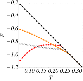
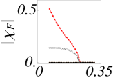
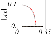
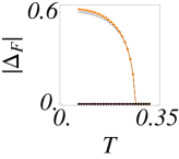
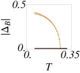
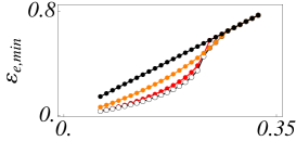
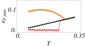
Figure 3: Left panel: Free energy for 1D, $U=4,x=0.1$ as a function of the temperature. The Black, White and Red dots follow the same color code as the phase diagrams. Central panel: Fermionic and bosonic order parameters as a function of temperature for each phase separately. Right Panel: Minimum energy as a function of temperature for the fermionic and bosonic bands.

(iii) For real physical systems described approximately by the Hubbard Hamiltonian other small coupling terms are expected that can qualitatively change the phase diagram locally. Different stable solutions that are not global minima will be considered elsewhere and are listed in the Appendix.

III Mean Field Phase Diagram for Hubbard chain and square lattice

A MF treatment of the original electron problem is not expected to be a good approximation for the one-dimensional case. However, it is interesting to construct a MF treatment in terms of new operators and to test the differences with the existing exact results and the domain of validity of the present treatment. It also permits to have a generic idea of the phase diagram and of the different phases present in higher dimensions.

In the case of the 1d Hubbard model we present some of the MF solutions obtained numerically solving the MF Eqs. (15-17) on a $200$ site chain. The results were obtained as follows: for a chosen point of the parameter space $U-T-x$ we generated several random trial solutions and used them as a starting point to our numerical routine. We obtained several different solutions unrelated by gauge transformations; however, just 4 of these solutions are relevant for the range of parameters considered here. The other solutions have very high values of the free energy or are “unphysical”. These 4 solutions were extended to the rest of the $U-x-T$ parameter space using as initial conditions a nearby converged solution. The four physical MF solutions differ by the existence of non-zero hopping and pairing terms. Fig. 1 shows the phase diagram $x-T$ for different values of $U$ and Fig. 2 the phase diagram $U-T$ for $x=0.1$. In these figures the results are presented on a finite mesh of points in the $x-T$ or $U-T$ planes.

For the two dimensional case we present the most stable MF solutions obtained numerically by solving the MF Eqs. 15-17 on a $16\times 16$ square lattice. The results were obtained as follows: for a chosen point of the parameter space $U-T-x$ we generated 1000 random initial conditions and used them as a starting point to our numerical routine. From this 1000 initial conditions 30 different solutions, non gauge equivalent, were found to converge. After this first step the 30 different solutions were extended to the rest of the $U-x-T$ parameter space using as initial conditions a nearby converged solution. This procedure is tedious since the convergence of the solutions is not always easy and some of them do not converge even if the difference in the parameters is small. Finally for each point in the $U-x-T$ space (again defined on a finite mesh) the solution with smallest free energy was found. Note that we did not impose any particular symmetry to solve the MF equations, the only assumption being translational invariance ($\boldsymbol{Q}_{r,\delta}=\boldsymbol{Q}_{\delta}$), in order to diagonalize the system in momentum space. That fact explains the proliferation of solutions of the MF equations.

III.1 Description of the Phase Diagram

Generically the phases found solving the MF solutions are characterized as follows:

- Phase (1) Conducting phase characterized by $\chi\neq 0,\ \Delta=0$ (Red): the spins are gapless and the charge degrees of freedom present a gap of the order of the temperature, which closes at $T=0$.

- Phase (2) $\chi=0,\ \Delta\neq 0$ phase (Orange), gapped for both degrees of freedom. Since it appears near $x=0$ it is tempting to identify this phase as an insulating antiferromagnet.

- Phase (3) $\chi\neq 0,\ \Delta\neq 0$ phase (White): precursor of the superconductor, in this phase there exists spin singlet formation but the charge motion is incoherent since no condensation was allowed. If we had imposed $\left\langle e_{k=0}\right\rangle=Z$ this phase would split in two sub-phases analog to the pseudogap and superconducting phases in Lee et al. (2006).

- Phase (4) High energy phase (Black): is an incoherent phase where all correlations are zero.

III.2 Characterization of the Phases

Our numerical results in one and two dimensions show that the $\chi=0,\ \Delta\neq 0$ (Orange) phase is dominant in the low doping region up to a temperature that decreases with U. In the 1D case this phase extends to the under-doped region and interfaces with the $\chi\neq 0,\ \Delta=0$ (Red) phase, present at higher doping, by a small finite-energy region where $\chi\neq 0,\ \Delta\neq 0$ (White phase). In 2D the $\chi=0,\ \Delta\neq 0$ (Orange) phase is numerically unstable and we could only find it for zero doping. The $\chi\neq 0,\ \Delta\neq 0$ phase appears also in the high doping regime at low $T$. In 1D the size of this region grows clearly with U, however, in 2D this is not clear but is definitely present at low energy. At very low $T$ the most stable solution is the Red phase ($\chi\neq 0;\Delta=0$) except at half-filling.

One-dimensional case

Figure 3 shows the free energy of the Hubbard chain for the four MF solutions when $U=4,x=0.1$ as a function of the temperature. At low temperature the $\chi\neq 0$ (Red) phase has a lower free energy and there is a first order phase transition with increasing temperature as the $\chi\neq 0;\Delta\neq 0$ phase becomes less energetic. At higher temperatures two second order phase transitions occur: first, for $T\simeq 0.23$, $\chi$ decreases to zero as the $\chi\neq 0;\Delta\neq 0$ joins the $\chi=0;\Delta\neq 0$ solutions; the second phase transition occurs for $T\simeq 0.27$ when $\Delta$ vanishes (see Fig. 3- central panel).

In the right panel of the same figure we show the minimum energy of the various bands as a function of temperature for the various phases. At low temperature where the Red phase is the most stable the fermionic bands are gapless. This phase is always gapless up to the point where it merges with the fully incoherent (black) phase. In the other phases the fermions are gapped (note that the spin spectrum in the Orange and White phases is almost the same). On the other hand, the bosonic (charge) spectrum is always gapped except at zero temperature.

Considering for instance $U=4,T=0.01$ we may as well analyze the results as a function of doping. At zero doping both $\chi\neq 0;\Delta\neq 0$ and $\chi=0;\Delta\neq 0$ coincide, this degeneracy is lifted for finite doping (in a very narrow region) and the $\chi\neq 0:\Delta\neq 0$ phase presents the minimal value of the free energy. From $x\simeq 0.1$ to $x\simeq 0.5$ there is an intermediate phase $\chi\neq 0;\Delta=0$ delimited by two first order transitions. For higher doping the $\chi\neq 0;\Delta\neq 0$ regains the minimal value of the free energy.

The hopping and pairing correlation functions

$$\chi_{F}(r) = \left\langle\mathit{s}_{r,1}^{\dagger}\mathit{s}_{0,1}+\mathit{s}_{r,-1}^{\dagger}s_{0,-1}\right\rangle_{0},$$

$$\Delta_{F}(r) = \left\langle\mathit{s}_{r,1}\mathit{s}_{0,-1}-\mathit{s}_{r,-1}\mathit{s}_{0,1}\right\rangle_{0},$$

$$\chi_{B}(r) = \left\langle\mathit{d}_{r}^{\dagger}\mathit{d}_{0}-\mathit{e}_{r}^{\dagger}\mathit{e}_{0}\right\rangle_{0},$$

$$\Delta_{B}(r) = \left\langle\mathit{d}_{r}\mathit{e}_{0}+\mathit{e}_{r}\mathit{d}_{0}\right\rangle_{0},$$ (39)

are shown in Fig. 4 at two doping values $x=0.1,x=0.6$. Even if these correlation functions are not gauge invariant they can be quite useful to characterize the different phases. In particular one can clearly see the difference between the two disjoint $\chi\neq 0;\Delta\neq 0$ (White) ((3) and (3’)) regions. At lower doping $x=0.1$ we consider the three non-trivial solutions as a function of increasing temperature and at the higher doping ($x=0.6$) we consider the White and Red solutions. Both for the fermion and the boson hopping correlation functions the correlation length increases as the doping increases. Particularly the bosonic correlation function has a large correlation length. Analyzing the correlation length of $\Delta_{B}$ one clearly sees a long range correlation in the high doping regime possibly precursor of Bose-condensation and superconductivity. In the low doping region both the bosonic and the fermionic correlation functions have a smaller range consistent with a spin gapped state. In this regime the two correlation functions have similar range while at higher doping the charge correlation function has a much larger range compared to the spin correlation function.

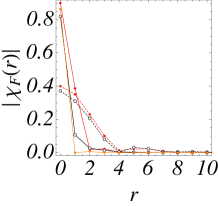
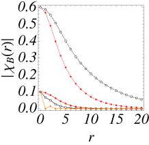
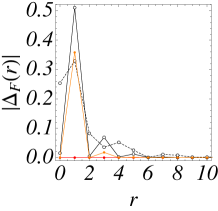
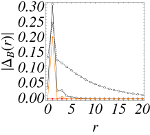
Figure 4: Hopping and pairing correlations as a function of the distance in 1D, computed for the three non-trivial MF phases with $U=4$. Red(full): Phase $\chi\neq 0,\Delta=0$ computed for $T=0.10,x=0.1.$ Red(dashed): Phase $\chi\neq 0,\Delta=0$ computed for $T=0.15,x=0.6$. White: Phase $\chi\neq 0,\Delta\neq 0$ computed for $T=0.19,x=0.1.$ White (dashed) : Phase $\chi\neq 0,\Delta\neq 0$ computed for $T=0.08,x=0.6.$ Orange: Phase $\chi=0,\Delta\neq 0$ computed for $T=0.24,x=0.1.$

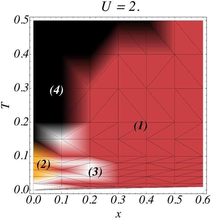
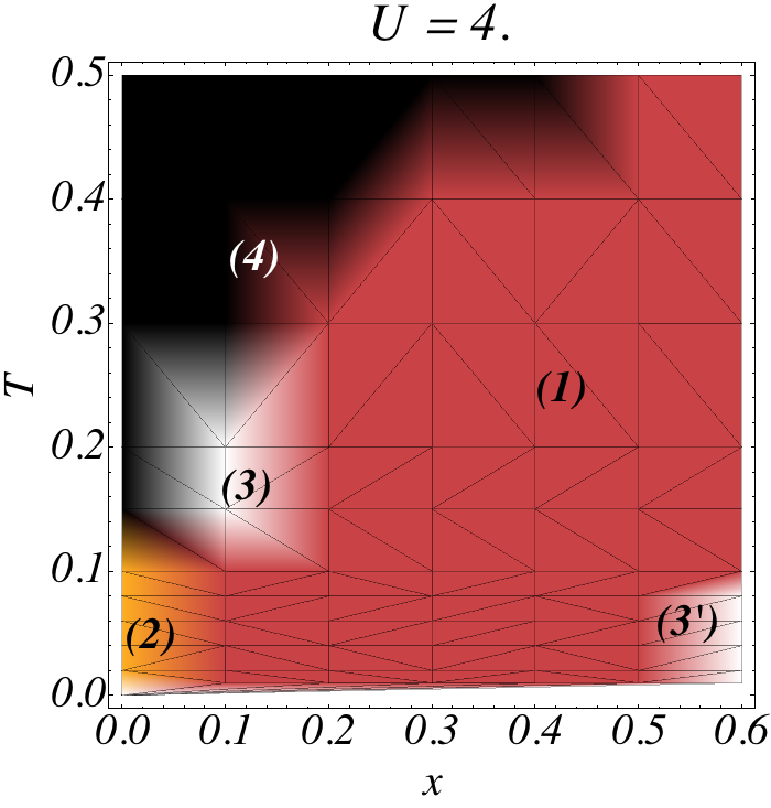
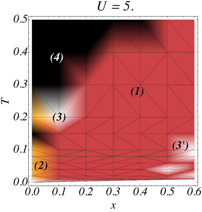
Figure 5: Mean field phase diagram in the $x-T$ plane as a function of $U$ for a $16\times 16$ square lattice. The colors represent the different types of solution minimizing the free energy: (1) $\chi\neq 0,\,\Delta=0$ (Red); (2) $\chi=0,\,\Delta\neq 0$ (Orange); (3) $\chi\neq 0,\,\Delta\neq 0$ (White); $\chi,\Delta=0$ (Black). The calculated points are placed in the nodes of the mesh, the colors plotted between nodes are interpolated.

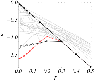
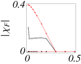
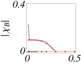
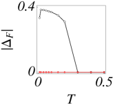
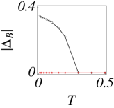
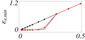
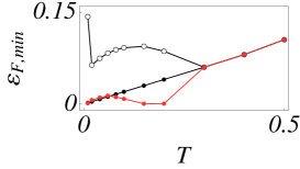
Figure 6: Left Panel: Free energy for $U=4,x=0.1$ as a function of the temperature. The Black, White and Red dots follow the same color code as the phase diagrams. The Gray lines in background are the free energies of the rest of the converged solutions (most of which are unphysical, see main text). Central panel: Fermionic order parameters as a function of temperature for each phase separately, note that solutions that minimize the free energy are symmetric under rotations of the lattice. Right Panel: Minimum of the one particle excitation energies of the diagonalized bosonic and fermionic MF Hamiltonians.

Two-dimensional case

The phase diagram for the square lattice is shown in Fig. 5. The free energy for the square lattice as a function of the temperature is shown in Fig. 6 for $U=4,\ x=0.1$. The low temperature state is, as in the 1D case, given by the phase $\chi\neq 0,\Delta=0$ (Red). There is a first order phase transition to the solution $\chi\neq 0;\Delta\neq 0$ (White) as the temperature increases. However contrary to the 1D case there is only one second order phase transition for higher temperature where both hoppings and pairings vanish at the same time. Both phases (Red and White) present gapless bosonic (charge) excitations (see Fig. 6-Right panel) but the minimum of the bosonic 1-particle excitations is located at $k=\left\{0,0\right\}$ and $k=\left\{\pi,\pi\right\}$ respectively. Furthermore the $\chi\neq 0,\Delta=0$ (Red) phase has no spin gap (see Fig. 6-Right panel, here we believe that the oscillations are due to finite size effects). Also note that contrarily to the one-dimensional case the fully incoherent phase has a fermionic (spin) gap smaller than the White phase. However, the White phase is the most stable one for dopings between $0.15-0.3$ which indicates the presence of a spin gap (pseudogap) in this region.

As a function of doping the free energy is minimal at half filling for the state $\chi=0;\Delta\neq 0$ (Orange). This state is the zero doping limit of the state $\chi\neq 0;\Delta\neq 0$ (White) where the values of $\chi$ vanish. Moreover one observes a first order phase transition to the state $\chi\neq 0,\Delta=0$ (Red) as the doping is increased. For $U=2$ this arises away from half-filling resulting in two consecutive phase transitions with increasing values of $x$, the first from $\chi=0;\Delta\neq 0$ (Orange) to $\chi\neq 0;\Delta\neq 0$ (White) is of second order, and the second from $\chi\neq 0;\Delta\neq 0$ (White) to$\chi\neq 0,\Delta=0$ (Red) is of first order. For $U=4,5$ only the first order transition is observed arising at $x=0$ between phases $\chi=0;\Delta\neq 0$ (Orange) and $\chi\neq 0,\Delta=0$ (Red). For still higher doping and sufficiently strong $U$ there is another first order transition back to the state $\chi\neq 0;\Delta\neq 0$ (White).

III.3 Magnetic Properties

By construction of the present MF decoupling there is no sub-lattice magnetization. Moreover since there is no anti-ferromagnetic term in the Lagrangian the usual d-wave solutions of the $t-J$ model are absent. Indeed, for two dimensions, the solutions with smallest free energy were found to be invariant under lattice rotation. However, a collection of other solutions that break rotational symmetry of the lattice where found which are not the minima of the free energy, as shown in the Appendix. The Spin-Spin correlation $\left\langle\mathbf{S}_{r}.\mathbf{S}_{r^{\prime}}\right\rangle$ functions, at the MF level, are exponentially decaying with the distance and negative for $r\neq r^{\prime}$ at finite $T$ and for all non-trivial phases. This is compatible with the RVB picture where there is singlet formation for $r$ and $r^{\prime}$ not nearest neighbors.

III.4 Charge Properties

Using that

$$c_{\mathbf{k},\sigma}=\frac{1}{\sqrt{V}}\sum_{\mathbf{q}}\left(e_{\mathbf{q}}^{\dagger}s_{\mathbf{q}+\mathbf{k},\sigma}+\sigma s_{\mathbf{q},-\sigma}^{\dagger}d_{\mathbf{q}+\mathbf{k}}\right)$$ (40)

we can write the Green’s function as

$$\langle T_{\tau}c_{k,\sigma}(\tau)c_{k,\sigma}^{\dagger}\rangle=\frac{1}{V}\sum_{\mathbf{q}}$$

$$\left\{\left\langle\mathit{e}_{q}^{\dagger}(\tau)\mathit{e}_{q}\right\rangle_{0}\left\langle\mathit{s}_{k+q,\sigma}(\tau)\mathit{s}_{k+q,\sigma}^{\dagger}\right\rangle_{0}\right.$$

$$+\left\langle\mathit{d}_{q}(\tau)\mathit{d}_{q}^{\dagger}\right\rangle_{0}\left\langle\mathit{s}_{q-k,-\sigma}^{\dagger}(\tau)\mathit{s}_{q-k,-\sigma}\right\rangle_{0}$$

$$+\sigma\left\langle\mathit{d}_{q}(\tau)\mathit{e}_{-q}\right\rangle_{0}\left\langle\mathit{s}_{q-k,-\sigma}^{\dagger}(\tau)\mathit{s}_{k-q,\sigma}^{\dagger}\right\rangle_{0}$$

$$\left.+\sigma\left\langle\mathit{e}_{-q}^{\dagger}(\tau)\mathit{d}_{q}^{\dagger}\right\rangle_{0}\left\langle\mathit{s}_{k-q,\sigma}(\tau)\mathit{s}_{q-k,-\sigma}\right\rangle_{0}\right\}$$ (41)

For the case with no pairing correlations between fermions and considering the bosons to be condensed leads to a Fermi liquid-like behavior for the electron Green’s function where the pole like structure of the coherent part is determined by the spectrum of the fermions and the condensates give the Z renormalization factor. Since condensation was not allowed our phase diagram apparently misses two phases of Ref.Lee et al. (2006) away from $T=0$: the normal Fermi liquid phase and the superconducting (SC) phase. In one dimension the phase ($\chi\neq 0,\ \Delta=0$) has a charge (bosonic) gap that goes to zero with the temperature and a vanishing fermionic gap (see Fig. 3). However, in two dimensions both gaps are zero in this phase (see Fig. 6). Therefore at least at zero temperature there will be Bose condensation and assuming a small interlayer coupling we may have Bose condensation at finite temperature. Here we consider that the condensation temperature is smaller than the considered range of temperatures. Note that a conductor state is found for the $\chi\neq 0,\ \Delta=0$ phase as seen ahead in the spectral function where the spectral weight goes down to zero energy. For the other nontrivial phases a spin gap is present at low temperatures and one expects an insulator state. This is also corroborated by the spectral function analysis where no substantial spectral weight is seen near zero energy.

No condensation implies that the “superfluid” density $\rho_{a}(k)=V^{-1}\left|\left\langle a_{k}a_{k}\right\rangle_{0}\right|$ ($a=d,e$) is zero for all $k$ and thus no SC correlations are present. Note that the symmetry of the SC gap is given by the SC correlation functions of the $s$ particles. The superconductor correlation function, at the MF level, is given by

$$\left\langle c_{k,1}^{\dagger}c_{-k+p,-1}^{\dagger}\right\rangle=\sum_{K}\delta_{p,2K}$$ (42)

$$\left[\left\langle s_{k-K,1}^{\dagger}s_{-k+K,-1}^{\dagger}\right\rangle_{0}\frac{\left\langle e_{-K}e_{-K}\right\rangle_{0}}{V}\right.$$

$$- \left.\left\langle s_{-k+K,-1}s_{k-K,1}\right\rangle_{0}\frac{\left\langle d_{K}^{\dagger}d_{K}^{\dagger}\right\rangle_{0}}{V}\right]$$

$$= 0$$

where $\delta_{k,0}$ is $2\pi$ periodic in $k$ so the sum over $K$ is reduced to two factors. However for the phases where $\Delta\neq 0$ the anomalous spin correlation functions (defined in Eq. 39) are finite, which can be seen as a precursor for superconductivity.

IV Spectral function

(a)
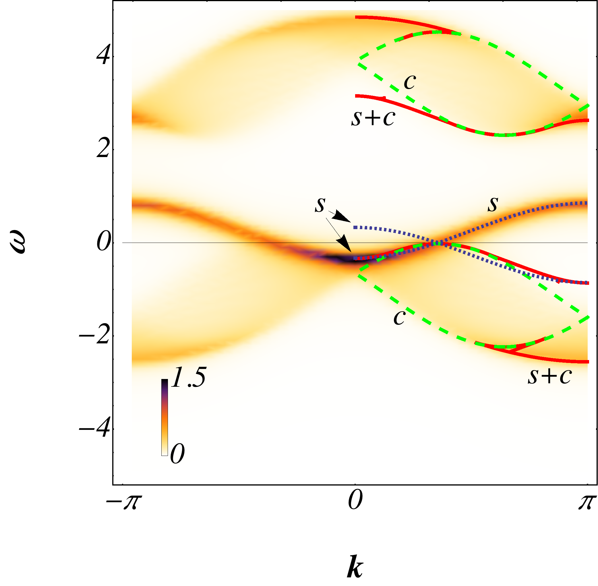
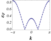
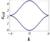
(b)
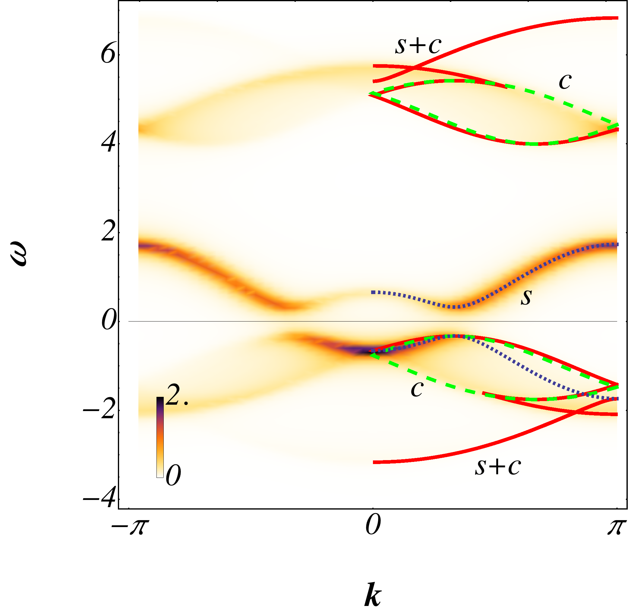
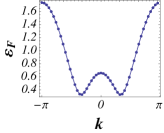
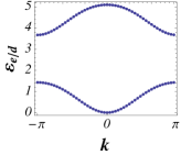
(c)

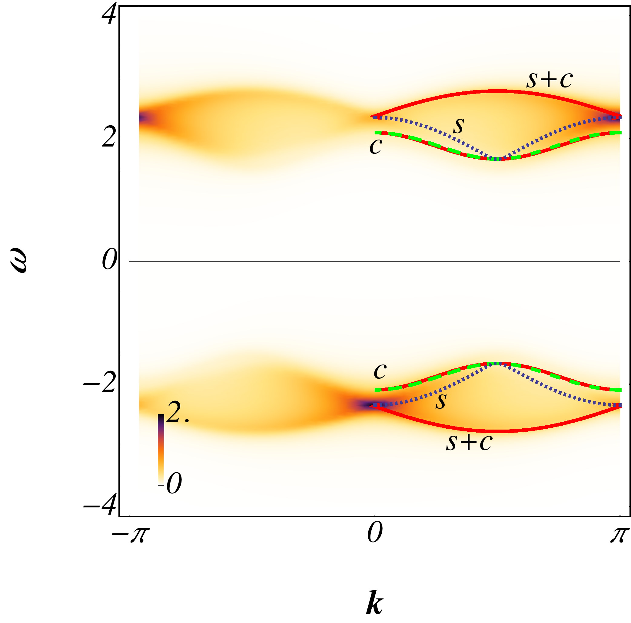
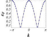
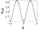
Figure 7: Spectral function and single particle energies for the Hubbatd chain: (a) Phase $\chi\neq 0;\ \Delta=0$ computed for $U=4;\ x=0.3;\ T=0.06$. (b) Phase $\chi\neq 0;\ \Delta\neq 0$ computed for $U=4;\ x=0.5;\ T=0.06$. (c) Phase $\chi=0;\ \Delta\neq 0$ computed for $U=4;\ x=0;\ T=0.06$. The $U-x-T$ parameters were chosen such that each solution is a minimum of the free energy. Colored lines are plotted along regions of considerable spectral weight and are obtained as follows: (Dark Blue, dotted line) varying the momentum of the fermions while keeping the momentum of the bosons to its minimal energy; (Green, dashed line) fixing the fermion energy to its minimal value and changing the momentum of the bosons; (Red, solid line) requiring that both excitations have equal velocities.

An efficient way to obtain information about the excitation spectrum of a strongly correlated system is through the spectral function. This is defined as the imaginary part of the Green’s function and is directly measurable through photoemission experiments. For the theory considered here the electron spectral function at the MF level can be written as

$$A_{\sigma}(\omega,k) = \frac{1}{V}\sum_{q}\left[\delta(\omega+\omega_{e,q}+\omega_{F,-q-k})\left[1+\mathit{n}_{b,e}(q)-\mathit{n}_{f}(-q-k)\right]\left|u_{F,q+k}v_{B,-q}+u_{B,-q}v_{F,q+k}\right|^{2}\right.$$ (43)

$$+\delta\left(\omega-\omega_{d,q}+\omega_{F,q-k}\right)\left[\mathit{n}_{f}(q-k)+\mathit{n}_{b,d}(q)\right]\left|u_{B,q}u_{F,k-q}+v_{F,k-q}\bar{v}_{B,q}\right|^{2}$$

$$+\delta\left(\omega-\omega_{d,q}-\omega_{F,k-q}\right)\left[1+\mathit{n}_{b,d}(q)-\mathit{n}_{f}(k-q)\right]\left|u_{F,k-q}v_{B,q}-u_{B,q}v_{F,k-q}\right|^{2}$$

$$\left.+\delta\left(\omega+\omega_{e,q}-\omega_{F,q+k}\right)\left[\mathit{n}_{f}(q+k)+\mathit{n}_{b,e}(q)\right]\left|u_{B,-q}u_{F,q+k}-v_{F,q+k}\bar{v}_{B,-q}\right|^{2}\right]$$

and has information about the excitation spectra and their spectral weights.

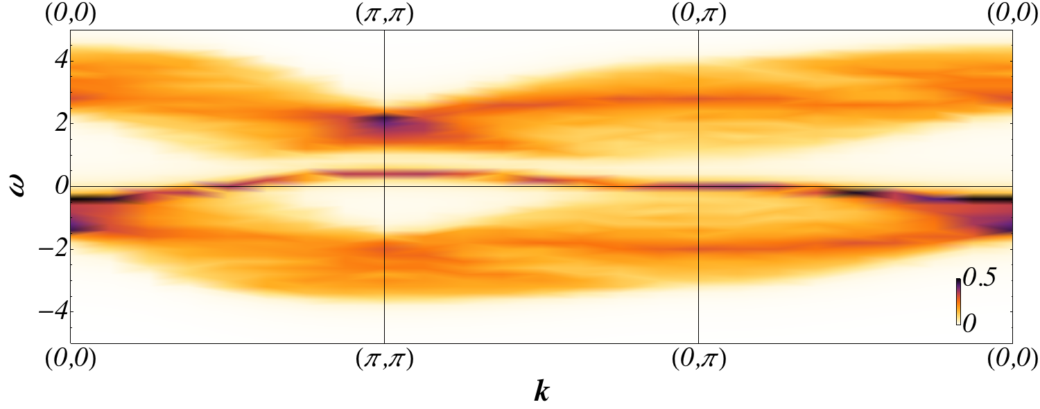
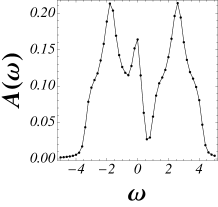
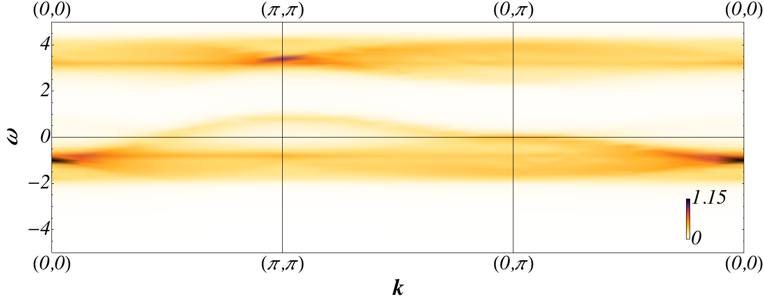
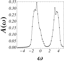
Figure 8: Spectral function and density of states computed at the MF level for a square lattice $16\times 16$. Upper panel: phase $\chi\neq 0,\Delta=0$ ($U=4,T=0.01,x=0.1$). Lower panel: phase $\chi\neq 0,\Delta\neq 0$ ($U=4,T=0.2,x=0.1$)

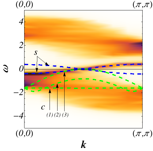
Figure 9: Spectral function for the square lattice for the phase $\chi\neq 0,\Delta=0$ along the nodal line. The lines green are obtained fixing the fermion momentum at the Fermi level along the directions $(1)=(\pi,0);\ (2)=(\pi/2,\pi/2);\ (3)=(0,\pi)$ and varying the momentum of the bosons. The blue lines are obtained fixing the bosons energy to be minimal (corresponding to zero momentum) and varying the fermionic momentum.

Experiments for one-dimensional insulators and conductors have shown the fractionalization of the electronic degrees of freedom inside the strongly correlated system. For instance experimental results for the one-dimensional conductor TTF-TCNQ have been interpreted using the Bethe ansatz solution showing clearly the traits of the spinon and holon branches associated with the spin and charge degrees of freedom (see Fig. 9 in Sing et al. (2003) and Figs. 1 in Carmelo et al. (2004b); Bozi et al. (2008)). In the context of the high-temperature superconductors similar results have been obtained for the spectral function in Graf et al. (2007); Damascelli et al. (2003). These results have also been interpreted in terms of some fractionalization of the degrees of freedom in a way similar to the one-dimensional case.

Fig. 7 shows the spectral function for the one-dimensional case computed at the MF level for the three non-trivial MF solutions. The regions of larger spectral weight correspond to three different processes. Two of those processes can be interpreted as the fractionalization of the electron since the fermions or the bosons (Blue or Green respectively) are fixed to the minimum value of their energy and the other species is allowed to move along its energy band. The high spectral weight of such regions is also observed in the spectral function computed based on the exact solution of the Hubbard model in 1D (REF). These are the so-called spectral lines "c" and "s" in refs. Sing et al. (2003); Carmelo et al. (2004b); Bozi et al. (2008). The third process can be interpreted as propagation of an "electron-like" degree of freedom (Red) since it corresponds to a boson and a fermion with the same velocity propagating together. These processes typically define the boundary lines of the region with a (nearly) non-vanishing spectral weight.

Consider first the top panel of Fig. 7 and the negative energy region corresponding to photoemission. In the regions of higher spectral weight at low energies we see that the lowest energy branch (s branch) is obtained fixing the bosons at their lowest energy and changing the fermionic (spin) particles along their bands. It is therefore a spin branch. Below this line at higher energy (recall that by definition $\omega<0$ for photoemission and therefore higher energies are more negative) there is a line that is obtained fixing the fermion at the Fermi surface and changing the boson energy along its band. It is therefore a charge (holon) band (c branch). These two lines are clearly separated as in the exact description from the Bethe ansatz and the experimental results Bozi et al. (2008). They merge at the Fermi level as in the exact solution. Note that in the region of high spectral weight there is a contribution from a line obtained taking the velocities of the fermions and bosons as equal. This means an "electronic-like" excitation. For larger momenta spin and a charge branch also emerge as in the exact solution. We also show the inverse photoemission spectra (positive energies) including the lowest and the upper Hubbard bands. In this phase there is a finite spectral weight at the Fermi energy which implies a conducting phase. This is consistent with the gapless fermionic band and the nearly gapless bosonic lowest band.

In the middle panel we consider the phase where both the hoppings and gap functions are finite (White phase). In this case the spins have a gap and the bosons are nearly gapless. The spectral function has now a pseudogap at the Fermi level since there is a small spectral weight. The finite energy structure is however quite similar to the fully conducting phase. Note that another contribution to this region is obtained fixing the fermion energy to its minimal (finite) value and changing the momentum of the bosons (nearly gapless). Note again that in the region of high spectral weight there is again a contribution from a line obtained taking the velocities of the fermions and bosons as equal.

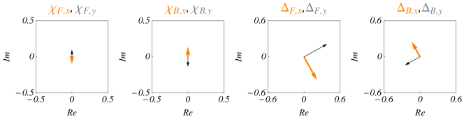
Figure 10: This figure shows how the results displayed in Fig. 11 should be interpreted.

Finally, in the lower panel we consider the Orange solution where the hopping parameters vanish and the gap functions are finite. In this case both the fermions and the bosons are gapped and the spectral function has a large gap. Also, the results are presented at half-filling and therefore the system is an insulator, as expected from the exact solution.

The spectral function and density of states

$$A(\omega)=\frac{1}{2}\frac{1}{V}\sum_{k,\sigma}A_{\sigma}(\omega,k)$$ (44)

for the square lattice are shown in Figs.8 and 9. For the $\chi\neq 0,\Delta=0$ (Red) phase it presents the same qualitative features as the one dimensional case. Namely a strong spectral weight is observed due to excitations corresponding to an empty site at $k=0$ and a spinon that carries the momentum of the physical electron (s branch). Excitations for which the spinon is taken at the Fermi surface and the holon carries the difference of momenta presents also some spectral weight (Green lines of Fig.9). Fig.9 shows Green lines (c branches) corresponding to the spinon momentum at the Fermi surface in the direction $(0,\pi),(\pi,\pi),(\pi,0)$ directions. The line reaching the Fermi energy corresponds to a fermion with momentum in the $(0,0)-(\pi,\pi)$ segment. This scenario of two spectral lines leaving the Fermi-surface of the spinons is also obtained by other recent approaches Phillips et al. (2009). The results for the White phase show a pseudogap structure as shown in the density of states $A(\omega)$.

V Discussion

We have extensively explored translationally invariant MF solutions of the Hubbard model for a one dimensional chain and for a square lattice using an electron representation introduced in Zou and Anderson (1988) and a MF decoupling in terms of link variables. In two dimensions this includes non-trivial symmetries of the MF solutions as well as nematic (translationally invariant but not rotationally invariant) and quasi-1D phases (but no flux phases). Despite all the freedom in the choice of solutions, the ones that minimize the free energy were found to be invariant under lattice rotations. However, in some phase space regions, the free energy difference between these less conventional phases (non rotationally invariant) and the symmetric ones (rotationally invariant) where found to be quite small signaling a possible stabilization of such phases by some extra coupling in the Hamiltonian. The symmetric phases where classified according to the MF order parameters and their physical properties where obtained.

Generically we found a gapped phase for both fermionic and bosonic (spinons and holons) degrees of freedom for zero doping. Contrarily to the 2D case, where this phase was only found for half filling, in the 1D case this phase extends to finite doping at finite temperatures and its size in the $T-x$ phase diagram decreases with $U$. This is in no contradiction with the exact solution for the ground state since for zero temperature only at half filling have we found this phase; the system is a conductor away from half filling. Although no magnetic order is obtained from the present MF ansatz this state is clearly a Mott insulator as one expects at half filling.

A conducting phase was found to be dominant for small and moderate doping from zero to quite high temperatures presenting the qualitative features of a RVB state. For the one dimensional conducting phase one can identify some of the features of the spectral function of Fig. 7 with the ones obtained from the exact Bethe Ansatz solution. In particular the lines carrying the most part of the spectral weight can be identified with three kinds of excitations. Two of them corresponding to a creation or annihilation of slave particles with different velocities. It is tempting to interpret such lines with fractionalization of the initial degrees of freedom. In the two dimensional case these lines are also obtained although they are not so clearly defined, in the sense that the spectral weight is not very pronounced for the c branches. Near the Fermi-energy such two lines are compatible with the description in Phillips et al. (2009). Lines where both slave particles have equal velocities are possible to draw only in the one dimensional case since they correspond to a surface in 2D. In this case they typically represent boundaries for the spectral weight. As in the former case one can try to interpret these lines as "electron-like" particles since they represent states where a slave boson and slave fermion travel together with the same velocity. In the region where the $\chi\neq 0,\Delta\neq 0$ phase appears the temperature is larger than the spin gap, the charge gap being zero. We note that in the one-dimensional case in the conducting phases the fermions are gapless and the bosons are gapped while in the square lattice the fermions are gapped and the bosons are gapless.

The results presented here describe the finite-energy finite-temperature phase diagram. At very low temperature a low energy theory where the lowest energy bosonic branch is condensed and the higher energy bosonic branch is frozen, will be presented elsewhere. It is particularly interesting in this low energy regime to consider frustrated lattices where it is expected that fractionalization will appear for either a conducting system, or for insulating systems where the possibility of spin liquids has been proposed.

Appendix A Mean Field Solutions

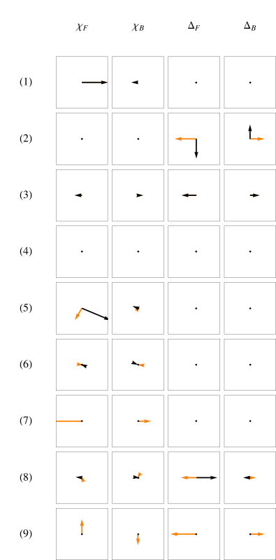
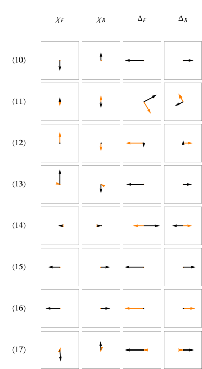
Figure 11: Mean Field Solutions

In this section we present a table with some of the solutions found for the square lattice, solving the MF equations. These solutions have low values of the free energy even though not absolute minima.

The results presented in Fig. 11 are obtained for $U=4,x=0.2,T=0.1$ for the two dimensional square lattice and are representative of the types of solutions found in other points of phase space. Solutions $(1),(3)$ and $(4)$ are the ones considered in the main text since they alternatively minimize the free energy depending on the considered phase space region: $(1)$ corresponds to the $\chi\neq 0,\Delta=0$ phase, $(3)$ corresponds to the $\chi\neq 0,\Delta\neq 0$ phase and $(4)$ is the incoherent phase where $\chi=0,\Delta=0$. Note that the solution $(2)$ referred in the main text corresponds to the zero doping limit of solution $(3)$, the one shown in Fig. 11 is also a solution of the type $\chi=0,\Delta\neq 0$ but it never presents the lowest free energy. The table entries are complex plane plots representing the MF parameters: columns 2 to 5 represent the values of $\chi_{F/B,\delta},\Delta_{F/B,\delta}$ for $\delta=\hat{e}_{x}$ (orange arrow) and $\delta=\hat{e}_{y}$ (black arrow); column 6 displays the values of $\mu$ (black arrow) and $i\lambda$ (orange arrow). The scales of the axes are shown in Fig. 10. We note some remarkable solutions obtained here: solution $(4)$ is an anisotropic $\chi\neq 0,\Delta=0$ solution; solutions $(9)$ and $(10)$ are related by a lattice rotation and represent one dimensional-like correlations where in one of the directions the MF parameters are zero; solution $(16)$ has $\chi\neq 0,\Delta=0$ in the $x$ direction and $\chi=0,\Delta\neq 0$ in the $y$ direction.

References

- Lieb and Wu (1968) E. H. Lieb and F. Y. Wu, Phys. Rev. Lett. 20, 1445 (1968).
- Takahashi (1972) M. Takahashi, Progress of Theoretical Physics 47, 69 (1972).
- Carmelo et al. (2004a) J. Carmelo, J. Roman, and K. Penc, Nucl. Phys. B 683, 387 (2004a).
- Harris and Lange (1967) A. B. Harris and R. V. Lange, Phys. Rev. 157, 295 (1967).
- Stein (1997) J. Stein, J. Stat. Phys. 88, 487 (1997).
- MacDonald et al. (1988) A. H. MacDonald, S. M. Girvin, and D. Yoshioka, Phys. Rev. B 37, 9753 (1988).
- Carmelo et al. (2000) J. M. P. Carmelo, N. M. R. Peres, and P. D. Sacramento, Phys. Rev. Lett. 84, 4673 (2000).
- Sing et al. (2003) M. Sing, U. Schwingenschlögl, R. Claessen, P. Blaha, J. M. P. Carmelo, L. M. Martelo, P. D. Sacramento, M. Dressel, and C. S. Jacobsen, Phys. Rev. B 68, 125111 (2003).
- Carmelo et al. (2004b) J. M. P. Carmelo, K. Penc, L. M. Martelo, P. D. Sacramento, J. M. B. L. dos Santos, R. Claessen, M. Sing, and U. Schwingenschlögl, Europhys. Lett. 67, 233 (2004b).
- Carmelo and Penc (2006) J. Carmelo and K. Penc, Eur. Phys. J. B 51, 477 (2006).
- Bozi et al. (2008) D. Bozi, J. M. P. Carmelo, K. Penc, and P. D. Sacramento, J. Phys.: Condens. Matter 20, 022205 (2008).
- Kotliar and Ruckenstein (1986) G. Kotliar and A. E. Ruckenstein, Phys. Rev. Lett. 57, 1362 (1986).
- Zou and Anderson (1988) Z. Zou and P. W. Anderson, Phys. Rev. B 37, 627 (1988).
- Dorin and Schlottmann (1992) V. Dorin and P. Schlottmann, Phys. Rev. B 46, 10800 (1992).
- Coleman (1984) P. Coleman, Phys. Rev. B 29, 3035 (1984).
- Östlund and Granath (2006) S. Östlund and M. Granath, Phys. Rev. Lett. 96, 066404 (2006).
- Dias and dos Santos (1992) R. G. Dias and J. M. B. L. dos Santos, J. Phys. I France 2, 1889 (1992).
- Peres et al. (2000) N. M. R. Peres, R. G. Dias, P. D. Sacramento, and J. M. P. Carmelo, Phys. Rev. B 61, 5169 (2000).
- Lee et al. (2006) P. A. Lee, N. Nagaosa, and X.-G. Wen, Rev. Mod. Phys. 78, 17 (2006).
- Leigh et al. (2007) R. G. Leigh, P. Phillips, and T.-P. Choy, Phys. Rev. Lett. 99, 046404 (2007).
- Choy et al. (2008) T.-P. Choy, R. G. Leigh, P. Phillips, and P. D. Powell, Phys. Rev. B 77, 014512 (2008).
- Phillips et al. (2009) P. Phillips, T.-P. Choy, and R. G. Leigh, Rep. Prog. Phys. 72, 036501 (2009).
- Vicente Alvarez et al. (1995) J. J. Vicente Alvarez, H. A. Ceccatto, and C. A. Balseiro, Phys. Rev. B 52, 14511 (1995).
- Kaplan et al. (1982) T. A. Kaplan, P. Horsch, and P. Fulde, Phys. Rev. Lett. 49, 889 (1982).
- Japaridze and Kampf (1999) G. I. Japaridze and A. P. Kampf, Phys. Rev. B 59, 12822 (1999).
- Strack and Vollhardt (1993) R. Strack and D. Vollhardt, Phys. Rev. Lett. 70, 2637 (1993).
- Arrachea and Aligia (1994) L. Arrachea and A. A. Aligia, Phys. Rev. Lett. 73, 2240 (1994).
- Dolcini and Montorsi (2002) F. Dolcini and A. Montorsi, Phys. Rev. B 66, 075112 (2002).
- Lee and Lee (2005) S.-S. Lee and P. A. Lee, Phys. Rev. Lett. 95, 036403 (2005).
- Brinckmann and Lee (2001) J. Brinckmann and P. A. Lee, Phys. Rev. B 65, 014502 (2001).
- Graf et al. (2007) J. Graf, G.-H. Gweon, K. McElroy, S. Y. Zhou, C. Jozwiak, E. Rotenberg, A. Bill, T. Sasagawa, H. Eisaki, S. Uchida, H. Takagi, D.-H. Lee, and A. Lanzara, Phys. Rev. Lett. 98, 067004 (2007).
- Damascelli et al. (2003) A. Damascelli, Z. Hussain, and Z.-X. Shen, Rev. Mod. Phys. 75, 473 (2003).