Equilibrium gas-liquid-solid contact angle from density-functional theory

Abstract

We investigate the equilibrium of a fluid in contact with a solid boundary through a density-functional theory. Depending on the conditions, the fluid can be in one phase, gas or liquid, or two phases, while the wall induces an external field acting on the fluid particles. We first examine the case of a liquid film in contact with the wall. We construct bifurcation diagrams for the film thickness as a function of the chemical potential. At a specific value of the chemical potential, two equally stable films, a thin one and a thick one, can coexist. As saturation is approached, the thickness of the thick film tends to infinity. This allows the construction of a liquid-gas interface that forms a well defined contact angle with the wall.

Keywords: contact angle; density-functional theory.

I Introduction

Wetting phenomena have received considerable attention over the past few decades (comprehensive and detailed reviews are given by Bonn et al. (2009) and de Gennes (1985)). Central to any description of wetting is the presence of a contact line which involves a three-phase conjunction (gas-liquid-solid). In the case of dynamic wetting the associated moving contact line problem is characterized by a stress singularity at the contact line. As a consequence, formulating this problem in the framework of conventional fluid mechanics leads to fundamental difficulties concerning the modeling of the contact line region Moffat (1963); Huh & Scriven (1971); E. B. Dussan & Davis (1974). Accordingly, a variety of models have been proposed to alleviate these difficulties and to address the behavior of the associated dynamic contact angle, with the most popular approaches being the replacement of the no-slip condition with a slip model or the elimination of the contact line all together with the use of a thin precursor layer. More recently, new approaches/theories have appeared, based e.g. on local diffuse-interface/Cahn-Hilliard-type approaches which, in general, cannot be rigourously justified. Other recent approaches include hybrid molecular-hydrodynamic simulations. However, the question of how to rigorously coarse grain from the micro- to the macro-scale and to accurately transfer molecular information to the macro-scale has not been adequately addressed as of yet.

The difficulties with the contact line region stem from the multi-scale nature of the problem. At the macroscale the usual laws of hydrodynamics apply. At the nanoscale intermolecular interactions, often described by molecular dynamics/Monte Carlo simulations, dominate. Yet, phenomena occurring at the nanoscale often manifest themselves at the macroscale (where individual molecules are not considered or equivalently the hydrodynamic laws consider a very large number of molecules at the same time). Despite drastic improvements in computational power, molecular simulations are still only applicable for small fluid volumes.

A compromise between conventional hydrodynamics and molecular simulations can be achieved by density-functional theory (DFT). On the one hand, DFT is able to retain the microscopic details of a macroscopic system at a computational cost significantly lower than that used in molecular simulations. On the other hand, DFT is rigorous compared to conventional phenomenological approaches. It is applicable for both uniform and non-uniform (density exhibits spatial variation) as well as confined systems (e.g. in the presence of a wall) within a self-consistent theoretical framework provided by the statistical mechanics of fluids. At the same time, substantial progress has been made in recent years in the development of realistic free-energy functionals which take into account the thermodynamic non-ideality attributed to the various intermolecular forces. The papers by Evans (1979), Tarazona (1985) and Argaman & Makov (2000) outline a DFT framework currently widely accepted by the statistical mechanics of fluids community and which has also been used successfully in describing equilibrium configurations in many different contexts, from fluids in pores to liquid crystals, polymers and molecular self-assembly.

Several studies have examined the equilibrium of liquids in contact with solids in different settings and in the framework of DFT/statistical mechanics of fluids. For example, Pismen (2002) adopted a DFT approach based on a free-energy functional proposed by Landau & Lifshitz (1980). This study focused primarily on a one-dimensional (1D) configuration, namely a liquid film in contact with a planar solid substrate but it did discuss contact lines; for a example it gave an approximate expression for the equilibrium contact angle obtained from the sharp-interface limit of the DFT approach adopted and for large distances from the solid substrate. Recently, Berim & Ruckenstein (2008a, b, 2009) adopted a DFT approach based on the framework described by Evans (1979), Tarazona (1985) and Argaman & Makov (2000) to calculate nanodrops on chemically/physically inhomogeneous inclined/planar substrates and to obtain the dependence of the contact angle of nanodrops on planar horizontal substrates on the parameters of the intermolecular interactions.

Our aim here is to provide a rigorous methodology for the treatment of contact lines. Our approach is also based on the DFT framework described by Evans (1979), Tarazona (1985) and Argaman & Makov (2000). We focus on the equilibrium of a fluid in contact with a planar solid substrate whose understanding is essential for the substantially more involved dynamics. We first examine in detail the 1D case of a liquid film in contact with the substrate. Particular emphasis is given on the bifurcation diagrams for the film thickness as a function of the chemical potential. This is a necessary step prior to understanding the more involved two-dimensional (2D) case, i.e. the three-phase contact line. We subsequently focus on the prewetting transition occurring at a specific value of the chemical potential where two equally stable films, a thin one and a thick one, coexist. The two thicknesses are connected through a ridge-like interface which is sufficiently smooth in the vicinity of the thin film for a long-range wall potential but it becomes steep there when the wall potential is a short-range one. When the co-existence value of the chemical potential equals to the saturation one, the thickness of the thick film tends to infinity. This is the case of a liquid wedge in contact with the solid substrate and with a well-defined three-phase contact line a few molecular diameters from the substrate. The wedge seems to persist for all distances from the substrate. Hence, even though DFT is a microscopic approach, it allows for the construction of a macroscopic quantity such as contact angle. Moreover, unlike macroscopic approaches e.g. Young’s equation which naturally require information on macroscopic parameters, such as the surface tensions between the different phases, DFT relies only on first principles, namely information related to intermolecular parameters. It also elucidates the structure of the three-phase contact line region and the precise role of fluid-fluid and fluid-solid (long-/short-range) interactions there.

II Problem definition

II.1 Setting

We consider part of a simple fluid inside a volume $\mathcal{V}$ in contact with a horizontal planar substrate as shown in figure 1. The system, whose boundary is denoted with the closed dotted line in the figure, is open, i.e. fluid particles can come in and out, and its surroundings are at temperature $T$ and chemical potential $\mu$. Depending on the conditions, the fluid can be in one phase (gas or liquid) or two phases. The fluid particles interact through a pair potential $\phi(r_{12})$, where $r_{12}$ is the distance between the centers of mass of the particles. The main effect of the substrate is to induce an external field $V(\mathbf{r})$ acting on the fluid particles with $\mathbf{r}$ the position vector of the inertial center of fluid particles. For the sake of simplicity, gravity is neglected. A Cartesian coordinate system $(x,y,z)$ is chosen such that $x$ and $y$ are parallel to the wall surface while $z$ is the outward-pointing coordinate normal to the wall. Of particular interest is the region around the solid/fluid interface.

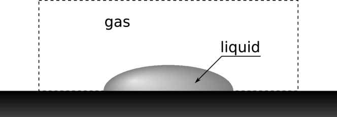
Figure 1: Sketch of the physical setting.

II.2 Density-functional theory of fluids

The equilibrium state of the system is characterized by the fluid density $n_{0}(\mathbf{r})$, in units of number of particles per unit volume (number density), defined as Evans (1979):

$$n_{0}(\mathbf{r})=<\sum_{i=1}^{N}\delta(\mathbf{r}-\mathbf{r}_{i})>$$ (1)

with $\mathbf{r}\in\mathcal{V}$. To obtain $n_{0}(\mathbf{r})$, we use elements from equilibrium statistical mechanics of fluids, in particular DFT. It has been shown that there exists a functional $\Omega[n]$, defined on a set of functions $n(\mathbf{r})$ compatible with the external potential $V(\mathbf{r})$, which has the property to be at a global minimum (for a given temperature, chemical potential and external potential) when $n(\mathbf{r})$ is equal to the equilibrium density profile $n_{0}(\mathbf{r})$ Evans (1979); Plischke & Bergersen (2006) (minimum principle). A second functional $F[n]$ can also be introduced such that $\Omega[n]$ reads:

$$\Omega[n]=F[n]+\int\!\text{d}\mathbf{r}\,n(\mathbf{r})(V(\mathbf{r})-\mu)\text{,}$$ (2)

where the integral is understood to be a volume one over $\mathcal{V}$. The intrinsic free energy and the grand potential of the system at equilibrium are then equal to $F[n_{0}]$ and $\Omega[n_{0}]$, respectively (such quantities can only be defined at equilibrium).

By using variational calculus, it can be easily shown that a necessary condition for a minimum of $\Omega[n]$ is:

$$\frac{\delta F[n]}{\delta n(\mathbf{r})}+V(\mathbf{r})=\mu.$$ (3)

This equation is supplemented by appropriate boundary conditions, i.e. the value of $n$ outside $\mathcal{V}$. In our case, the external potential $V(\mathbf{r})$ is due to the interaction between the fluid and the wall. Note that since our system is open (grand-canonical ensemble formalism), the total number of particles, $N$, is not given, but it is obtained instead once $n_{0}(\mathbf{r})$ is known: $N=\int d\mathbf{r}n_{0}(\mathbf{r})$. For simplicity, we drop the subscript 0 from $n$ hereinafter.

II.3 Fluid modeling

Several approximations for $F[n]$ have been proposed over the years. One which has proved to be successful in a number of cases is based on a perturbation approach. The basic idea is to split the pair potential $\phi(r_{12})$ into two terms: $\phi(r_{12})=\phi_{\text{r}}(r_{12})+\phi_{\text{p}}(r_{12})$. The first term, $\phi_{\text{r}}(r_{12})$, is a reference potential and usually corresponds to the harshly repulsive part of $\phi(r_{12})$, while the second term, $\phi_{\text{p}}(r_{12})$, acts as a “perturbation” to $\phi_{\text{r}}(r_{12})$ and is in general a slowly attractive potential. Such separation, which is reminiscent of the approach behind the van der Waals equation of state for gases and can thus be viewed as a generalization of this approach, is in general well-suited for treating dense fluids. Its underlying physical motivation is that the structure of a fluid is determined mainly by the repulsive forces. After some additional simplifications we have the following compact expression for $F[n]$ Evans (1979); Plischke & Bergersen (2006):

$$F[n]=F_{\text{r}}[n]+\frac{1}{2}\int\!\!\!\!\int\!\text{d}\mathbf{r}\text{d}\mathbf{r^{\prime}}\;n(\mathbf{r})n(\mathbf{r^{\prime}})\phi_{\mathrm{p}}(|\mathbf{r}-\mathbf{r^{\prime}}|)\text{.}$$ (4a)

The first term of equation (4a) accounts for $$\phi_{\text{r}}(r_{12})$$ and can be further simplified by using the co-called local density approximation:

$$F_{\text{r}}[n]=\int\!\text{d}\mathbf{r}n(\mathbf{r})f(n(\mathbf{r}))\text{,}$$ (4b)

where $f$ is the local free energy per particle of the reference fluid. The main simplification used to obtain the second term of equation (4a), which involves the attractive part of the interaction potential $\phi(r_{12})$, is to express the pairwise distribution function, i.e. the probability that two particles occupy the positions $\mathbf{r}_{1}$, $\mathbf{r}_{2}$, as the product of $\eta(\mathbf{r}_{1})$, $\eta(\mathbf{r}_{2})$ and the radial distribution function of the uniform reference fluid.

The decomposition of the pair potential in two parts can be done in different ways. In the Barker-Henderson approach for example Barker & Henderson (1967), the attractive part is,

$$\phi_{\text{p}}(r_{12})={}\begin{cases}\displaystyle 0\quad&\text{if $r_{12}<\sigma$}\\ \displaystyle 4\epsilon\left[{\left(\frac{\sigma}{r_{12}}\right)}^{12}-{\left(\frac{\sigma}{r_{12}}\right)}^{6}\right]\quad&\text{if $r_{12}>\sigma$,}\end{cases}$$ (5)

where $\epsilon$ is a parameter that measures the strength of the potential. Another possibility is the decomposition suggested by Weeks et al. (1971). Here we adopt the Barker-Henderson approach. The reference potential is then, $\phi_{\text{r}}=\phi-\phi_{\text{p}}$. However, to take full advantage of the perturbation technique, the reference system should be a well-known fluid: the preferred choice is often a hard-sphere fluid, whose bulk local free energy is well described by the Carnahan-Starling expression:

$$\beta f(T,n)=\ln(\Lambda^{3}n)-1+\frac{\eta(4-3\eta)}{{(1-\eta)}^{2}}$$ (6a)

where

$$\eta\equiv\frac{\pi}{6}d^{3}n\text{,}$$ (6b)

is the packing fraction, $d$ is the hard-sphere diameter, $\Lambda$ is the thermal de Broglie length and $\beta\equiv 1/(k_{\text{B}}T)$ with $k_{\text{B}}$ the Boltzmann constant. This means that $\phi_{\text{r}}$ is in fact approximated by a hard-sphere potential. The associated molecular diameter $d$, which appears in equation (6b) and hence (6a), can be linked to $\sigma$ and the reference part of the interaction potential Barker & Henderson (1967) but for simplicity we assume $d=\sigma$.

Instead of equations (4b) and (6a), one could use a more refined approach for a hard sphere fluid based on Rosenfeld’s fundamental measure theory Rosenfeld (1989). In general, this approach gives better results for the fluid density at small distances from the wall (a few molecular diameters) but requires a more involved computational treatment. Our aim here is to keep the formalism as simple as possible and yet retain the basic ingredients of the underlying physics.

By substituting equations (4a) and (4b) into equation  (3), we obtain:

$$\mu_{\text{r}}(n)+\int\!\text{d}\mathbf{r^{\prime}}n(\mathbf{r^{\prime}})\phi_{\mathrm{p}}(|\mathbf{r}-\mathbf{r^{\prime}}|)+V(\mathbf{r})=\mu$$ (7a)

where

$$\mu_{\text{r}}(n)\equiv{\left(\frac{\partial(nf(T,n))}{\partial n}\right)}_{T}\text{,}$$ (7b)

is the chemical potential of the reference system which in the case of a hard sphere fluid and using equation (6a) reads:

$$\beta\mu_{\text{r}}(n)=\ln\left(\Lambda^{3}n\right)+\frac{\eta(8-9\eta+3\eta^{2})}{{(1-\eta)}^{3}}\text{.}$$ (8)

When the external potential vanishes and the fluid is uniform, i.e. its density does not exhibit any spatial variation, equation (4a) combined with equation (4b), reduces to

$$F[n]=\mathcal{V}n\bar{f}(n)$$ (9a)

where

$$\bar{f}(n)=f(n)-\alpha n\quad\mbox{and}\quad\alpha=-\frac{1}{2}\int_{-\infty}^{+\infty}\!\!\!\text{d}\mathbf{r}\,\phi_{\text{p}}(|\mathbf{r}|)\text{.}$$ (9b)

Equation (7) is then an algebraic equation with parameters $T$ and $\mu$. Using for $f$ the expression given in equation (6a), the usual thermodynamics for liquid/gas systems applies. The solutions to equation (7) correspond to extrema of the functional $\Omega[n]$. There is one solution for $T>T_{\text{c}}$ and one to three solutions for $T<T_{\text{c}}$, where $T_{\text{c}}$ is the critical temperature ($\beta_{\text{c}}\equiv 1/(k_{\text{B}}T_{\text{c}}))$. In the latter case, there are two minima of equal depth for $\Omega$, at small and large densities, respectively, and a maximum at intermediate densities. The middle solution is unstable while the other two correspond to the liquid and gas bulk densities, denoted as $n_{\text{gas}}(T,\mu)$ and $n_{\text{liq}}(T,\mu)$, respectively, with $n_{\text{gas}}(T,\mu)<n_{\text{liq}}(T,\mu)$. The chemical potential at the gas/liquid transition will be denoted as $\mu_{\text{sat}}(T)$. The gas is the preferred state for $\mu<\mu_{\text{sat}}(T)$. At $\mu=\mu_{\text{sat}}(T)$ the gas and liquid bulk are at equilibrium while for $\mu>\mu_{\text{sat}}(T)$ the liquid is the preferred state. Note that in all cases considered here $T<T_{\text{c}}$ as close to the critical temperature thermal fluctuations, which are not taken into account in the DFT formalism adopted here, become significant.

II.4 Wall potentials

Three types of wall potential are considered in this study. All are attractive at large distances. The first two have the same infinite repulsive part but they differ in the range of the attraction term. The short-range potential reads,

$$V_{\text{SR}}(z)={}\begin{cases}\displaystyle\;+\infty\quad&\text{if $z<z_{\text{w}}$}\\ \displaystyle\;-\epsilon_{\text{w}}\exp\left(-\frac{z-z_{\text{w}}}{\sigma_{\text{w}}}\right)\quad&\text{if $z>z_{\text{w}}$}\end{cases}$$ (10a)

while for the long-range one we use,

$$V_{\text{LR}}(z)={}\begin{cases}\;+\infty\quad&\text{if $z<z_{\text{w}}$}\\ \displaystyle-2\epsilon_{\text{w}}{\left(\frac{1}{1+\frac{z-z_{\text{w}}}{\sigma_{\text{w}}}}\right)}^{3}\quad&\text{if $z>z_{\text{w}}$}.\end{cases}$$ (10b)

In these expressions, $$\epsilon_{\text{w}} \sigma_{\text{w}} z_{\text{w}}$$, and are three wall parameters; the first two are strictly positive and are related to the strength and range of the potentials. The expressions in equations 10a and 10b are useful in that they allow us to examine the effect of the wall attraction, and in particular its range, on the fluid equilibrium state. The last wall potential has a smooth repulsive part compared to the previous ones (i.e. it is non-infinite):

$$V_{\text{LJ}}(z)\!=\!\!{}\begin{cases}\;+\infty&\text{if $z<z_{\text{w}}$}\\ \displaystyle 2\epsilon_{\text{w}}\!\!\left[\frac{2}{15}{\left(\frac{\sigma_{\text{w}}}{z-z_{\text{w}}}\right)\!}^{9}\!\!-{\left(\frac{\sigma_{\text{w}}}{z-z_{\text{w}}}\right)\!}^{3}\!\right]\!\!\!\!&\text{if $z>z_{\text{w}}$}.\end{cases}$$ (10c)

It can be derived by considering that the wall is made of a uniform density of particles interacting with the fluid particles through a Lennard-Jones potential (see Appendix A). By setting $\sigma_{\text{w,LR}}=z_{\text{w,LR}}-z_{\text{w,LJ}}$ and $\epsilon_{\text{w,LR}}=(\sigma_{\text{w,LJ}}/\sigma_{\text{w,LR}})^{3}\epsilon_{\text{w,LJ}}$, the two last potentials have the same attractive part. Finally, it is also possible to have a purely repulsive wall with no attraction (a hard or dry wall),

$$V(z)={}\begin{cases}\;+\infty\quad&\text{if $z<z_{\text{w}}$}\\ \;0\quad&\text{if $z>z_{\text{w}}$}.\end{cases}$$

III 1D problem

III.1 Equations

In this section we assume that the system is invariant along the $x$ and $y$ directions and infinite in the $z$-direction. Equation (7a) then becomes:

$$\mu_{\text{r}}(n)+\int_{-\infty}^{+\infty}\!\text{d}z^{\prime}n(z^{\prime})\Phi_{\text{1d}}(z^{\prime}-z)+V(z)=\mu$$ (11a)

where

$$\Phi_{\text{1d}}(Z)=\int\!\!\!\!\!\int_{-\infty}^{+\infty}\!\!\!\text{d}x\,\text{d}y\,\phi_{\text{p}}\!\left(\sqrt{x^{2}+y^{2}+Z^{2}}\right);\quad Z\equiv z^{\prime}-z.$$ (11b)

The integral in (11b) can be performed analytically (see Appendix A). To solve numerically the integral equation (11) a simple iterative procedure can be employed based on a Picard scheme. The integral is first computed with the values of the density obtained from the previous iteration by using a simple trapezoidal rule and then the remaining terms are solved for $n$, which gives the new value for the density. We found that, with the exception of unstable solutions, this scheme is robust and allows the use of an initial guess which can be far from the solution. However, convergence tends to be slow after the first iterations. This can be greatly improved by using instead a more involved scheme based on a Newton procedure in which the Jacobian matrix is appropriately simplified. Details are given in Appendix B.

III.2 Density profiles

In figures 2 and 3, we present typical profiles obtained by solving equation (11). Figure 2 depicts the density profile of the fluid along the $z$-direction when $\mu=\mu_{\text{sat}}(T)$ in the absence of the wall. For this value of $\mu$, both bulk liquid and bulk gas are equally possible states ($\Omega$ has two variational minima of equal “depth” at $n_{\text{liq,gas}}$). The interface region is just a few molecular diameters thick. The location of the sharp interface, say $z_{\text{I}}$, can be obtained from the Gibbs dividing surface defined from $\int_{-\infty}^{z_{\text{I}}}(n_{\text{liq}}-n)\text{d}z=\int_{z_{\text{I}}}^{+\infty}(n-n_{\text{gas}})\text{d}z$.

Figure 3 shows profiles obtained when the wall is switched on and exerts a long-range attraction on the fluid molecules. In this case, $\mu<\mu_{\text{sat}}(T)$ so that the bulk gas is the more stable phase in the absence of the wall ($\Omega$ has a single variational minimum at $n_{\text{gas}}$). As $z\rightarrow+\infty$ the density tends to the density of the gas, $n_{\text{gas}}$, but near the wall the attractive potential induces a bump in the density profile. If $\mu$ is close enough to $\mu_{\text{sat}}(T)$ (solid line in figure 3), this bump is more pronounced while the fluid density in that area is roughly equal to the metastable liquid bulk density (corresponding to a local variational minimum of $\Omega$). A thin liquid film is effectively formed between the wall and the gas. It can only exist due to the attraction with the wall, in other words an attractive wall stabilizes a thin liquid film in contact with it. We also note the small oscillations in the density profile near the wall corresponding to adsorption of the liquid particles there. More pronounced oscillations would have been found in this area if the reference system of hard sphere fluid had been treated with a more refined model like the Rosenfeld fundamental measure theory mentioned earlier Rosenfeld (1989). Also, when a thin film is present, we observe that the interface between the film and the gas phase is very similar (although $\mu$ is different) to the profile given in figure 2 suggesting that in that case, the wall has little influence. In fact, as $\mu\rightarrow\mu^{-}_{\text{sat}}$, the thickness of the liquid film tends to infinity and we approach the case depicted in figure 2, i.e. it is like the wall is not even present (with the exception of course of the area close to it where the density oscillations occur).

For given external conditions of temperature and chemical potential, an illustration of the dependance of the density profile on the characteristics of the wall potential is shown in figure 4. We first note when comparing wall potentials $V_{\text{SR}}$ (dashed-dotted line) and $V_{\text{LR}}$ (dashed line), that the liquid film thickness in the first case is considerably smaller even though all wall parameters are identical and in particular the integrals between $z_{\text{w}}$ and $+\infty$ of the two wall potentials are the same. In contrast, when $z_{\text{w,LR}}=z_{\text{w,LJ}}+\sigma_{\text{w,LR}}$, wall potentials $V_{\text{LR}}$ (dashed line) and $V_{\text{LJ}}$ (solid line) yield similar profiles except near the wall. These two last profiles can be made even closer to each other, including the area close to the wall, by changing the value of $z_{\text{w,LR}}$ through $\sigma_{\text{w,LR}}$ (dotted line) and updating $\epsilon_{\text{w,LR}}$ accordingly. However, even if the profiles can become similar, important differences can still exist in the adsorption isotherms (cf next section).

Figure 2: Density in the vicinity of a liquid-gas interface for $\mu=\mu_{\text{sat}}$ at $T=0.7\,T_{\text{c}}$ in the absence of the wall. The domain size used in the computation is [0-50] and the number of points is 1000. The bulk liquid density is $n_{\text{liq}}d^{3}\approx 0.684$ and the bulk gas one is $n_{\text{gas}}d^{3}\approx 0.0178$.

Figure 3: Density profiles for $\mu<\mu_{\text{sat}}$ at $T=0.7\,T_{\text{c}}$ near an attractive wall. The wall potential is $V_{\text{LJ}}$ given by equation (10c) with parameters $\beta_{\text{c}}\epsilon_{\text{w}}=1.8$, $\sigma_{\text{w}}=1.25\,d$ and $z_{\text{w}}=0$. Solid line, $\mu-\mu_{\text{sat}}=-0.001k_{\text{B}}T_{\text{c}}$; dotted line, $\mu-\mu_{\text{sat}}=-0.01k_{\text{B}}T_{\text{c}}$. In the former case, $n_{\text{liq}}d^{3}\approx 0.684$ which is close to the value of the density for $z/d$ in the interval $[3,17]$.

Figure 4: Density profiles for $\mu-\mu_{\text{sat}}-0.001k_{\text{B}}T_{\text{c}}$ at $T=0.7\,T_{\text{c}}$ near an attractive wall. Solid line: wall potential $V_{\text{LJ}}$ with $\beta_{\text{c}}\epsilon_{\text{w}}=1.8$, $\sigma_{\text{w}}=1.25\,d$ and $z_{\text{w}}=0$; dashed line: wall potential $V_{\text{LR}}$ with $\beta_{\text{c}}\epsilon_{\text{w}}=1.8$, $\sigma_{\text{w}}=1.25\,d$ and $z_{\text{w}}=\sigma_{\text{w}}$; dotted line: wall potential $V_{\text{LR}}$ with $\beta_{\text{c}}\epsilon_{\text{w}}\approx 3.52$, $\sigma_{\text{w}}=d$ and $z_{\text{w}}=\sigma_{\text{w}}$; dashed-dotted line: wall potential $V_{\text{SR}}$ with $\beta_{\text{c}}\epsilon_{\text{w}}=1.8$, $\sigma_{\text{w}}=1.25\,d$ and $z_{\text{w}}=\sigma_{\text{w}}$.

III.3 Isotherms

Of particular interest is the dependence of the film thickness with respect to $\mu$ for a given $T$. This is crucial to understanding more involved configurations such as the contact angle case examined later. Because of the spatial variation of the density, it is in fact more relevant to consider an integral norm of the density, the “adsorption”, defined as

$$\Gamma=\int_{-\infty}^{z_{\text{I}}}\text{d}z\,n(z)+\int_{z_{\text{I}}}^{+\infty}\text{d}z\,(n(z)-n_{\infty})$$ (12)

where $z_{\text{I}}$ is the position of the dividing wall-fluid interface and $n_{\infty}$ is in the present case equal to $n_{\text{gas}}$ ($n=0$ as $z\rightarrow-\infty$). The bifurcation diagrams for the isotherms are constructed with a continuation procedure which also involves an extra equation/geometric constraint which links the continuation parameter $\mu$ and $n$ with the continuation step. Besides easily obtaining the density profiles for a wide range of values of $\mu$, this approach has the additional benefit that it allows the computation of unstable branches, which would have been more difficult if not impossible to obtain otherwise.

Typical isotherms for the wall potential $V_{\text{LJ}}$ in equation (10c) are depicted in figure 5. For very attractive walls (for example, the case $\beta_{\text{c}}\epsilon_{\text{w}}=3$ in figure 5) and $\mu<\mu_{\text{sat}}$, the adsorption $\Gamma$ is a monotonically increasing function of $\mu$; in particular, only one solution exists for a given value of $\mu$. At the saturation value $\mu_{\text{sat}}$, the bulk liquid phase becomes as stable as the bulk gas one and the adsorption goes to infinity. For less attractive walls, a multi-valued S-shaped loop in the isotherm appears for values of $\mu$ say in $[\mu_{-},\mu_{+}]$ and with three branches of solutions from which the middle one is always unstable (corresponding to variational maxima for $\Omega$). This loop is associated with the presence of a first-order phase transition with respect to the adsorption: for a certain value of $\mu\in[\mu_{-},\mu_{+}]$, three solutions exist, of which those in the lower and upper branches are equally stable (variational minima of $\Omega$ of equal “depth”), and consequently the system can adopt for that value of $\mu$ two different adsorptions or equivalently film thicknesses. This transition is often referred to as the “prewetting transition” and a Maxwell construction in the variables $(\mu,\Gamma)$ can be carried out to find the coexistence value $\mu_{\text{coex}}(T)$ of the chemical potential at which the two states have the same stability. For $\mu\in[\mu_{-},\mu_{\text{coex}}]$, the lower branch is stable and the upper branch one metastable ($\Omega$ has two variational minima but the one in the lower branch is “deeper”) while for $\mu\in[\mu_{\text{coex}},\mu_{+}]$ the upper branch is stable and the lower one metastable.

The value $\mu_{\text{sat}}$ imposes an upper bound on $\mu_{\text{coex}}$. We cannot have $\mu_{\text{coex}}\geq\mu_{\text{sat}}$ as a Maxwell construction in this region is not possible. As $\mu_{\text{coex}}\rightarrow\mu^{-}_{\text{sat}}$ we can have a Maxwell construction with a thin film equally stable with an almost infinite thick film, while for $\mu=\mu_{\text{sat}}$ the most stable state is that of a thin film on the lower branch as is the case when the wall is only slightly attractive (e.g. $\beta_{\text{c}}\epsilon_{\text{w}}=0.8$ in figure 5). This is the signature of a partial wetting situation. Complete wetting on the other hand occurs whenever $\mu_{\text{coex}}<\mu_{\text{sat}}$ and as $\mu\rightarrow\mu_{\text{sat}}$ on the upper branch. For a given value of $\epsilon_{\text{w}}$, one can usually go from a partial wetting case to a complete wetting one by changing the temperature.

Typical isotherms for the wall potentials $V_{\text{SR}}$ and $V_{\text{LR}}$ in equations (10a) and (10b) are shown in figures 6 and 7, respectively. The isotherms appear qualitatively similar to those in figure 5. The effect of the potential ranges, however, becomes apparent in the upper half of the figures as, for a given isotherm, $\mu$ tends to $\mu_{\text{sat}}$ as $\Gamma d^{2}$ goes to $+\infty$ much faster in the case of potential $V_{\text{SR}}$ than in the case of potential $V_{\text{LR}}$. It may also be worthwile to note the important differences in the bottom half of the figures even though the distance from the wall is small there (i.e. the potential range is less critical): the values of $\mu_{-}$, $\mu_{\text{coex}}$ and $\mu_{+}$ in the two cases differ significantly. This is confirmed in figure 8 where their dependance on the strength $\epsilon_{\text{w}}$ of the wall potentials is depicted. The intersection of $\mu_{\text{coex}}$ with the $x$-axis (i.e. the $\mu=\mu_{\text{sat}}$ axis) in figure 8 corresponds to the partial/complete wetting transition with respect to $\epsilon_{\text{w}}$. For weakly attractive walls ($\epsilon_{\text{w}}$ small), the wetting is partial and becomes complete for very attractive walls ($\epsilon_{\text{w}}$ large). In the present case, the transition occurs sooner for the short-range potential.

Note that independently of the situation, complete wetting or partial wetting, there is always a film (albeit very thin) in contact with the wall. After all, the wall is always attractive. If it were repulsive, i.e. a hard or dry wall, there would be no contact between the fluid and the wall.

Figure 5: Bifurcation diagram for $\Gamma$ as a function of $\delta\!\mu\equiv\mu-\mu_{\text{sat}}$, for the attractive wall with potential $V_{\text{LJ}}$ (equation (10c)), $z_{\text{w}}=0$ and $\sigma_{\text{w}}=1.25\,d$. The temperature is $T=0.7\,T_{\text{c}}$ and the dividing interface is located at $z_{\text{I}}=z_{\text{w}}$. The wall parameter $\beta_{\text{c}}\epsilon_{\text{w}}$ varies from 0.8 (right curve) to 3.0 (left curve) in steps of 0.1.

Figure 6: Bifurcation diagram for $\Gamma$ as a function of $\delta\!\mu\equiv\mu-\mu_{\text{sat}}$, for the attractive wall with potential $V_{\text{SR}}$ (Eq. (10a)), $z_{\text{w}}=0$ and $\sigma_{\text{w}}=1.25\,d$. The temperature is $T=0.7\,T_{\text{c}}$ and the dividing interface is located at $z_{\text{I}}=z_{\text{w}}$. The wall parameter $\beta_{\text{c}}\epsilon_{\text{w}}$ varies from 1.2 (right curve) to 3.4 (left curve) in steps of 0.1.

Figure 7: Bifurcation diagram for $\Gamma$ as a function of $\delta\!\mu\equiv\mu-\mu_{\text{sat}}$, for the attractive wall with potential $V_{\text{LR}}$ (equation (10b)), $z_{\text{w}}=0$ and $\sigma_{\text{w}}=1.25\,d$. The temperature is $T=0.7\,T_{\text{c}}$ and the dividing interface is located at $z_{\text{I}}=z_{\text{w}}$. The wall parameter $\beta_{\text{c}}\epsilon_{\text{w}}$ varies from 1.2 (right curve) to 3.4 (left curve) in steps of 0.1.

Figure 8: Special values ($\mu_{-}$, $\mu_{\text{coex}}$ and $\mu_{+}$) of the chemical potential as a function of $\epsilon_{\text{w}}$. The solid lines correspond to wall potential $V_{\text{SR}}$ and the dotted lines to wall potential $V_{\text{LR}}$. The remaining parameters are the same as in figures 6 and 7.

III.4 Square gradient approach

A substantial simplification to equation (4a) can be achieved if we assume that $n(\mathbf{r})$ varies smoothly in the range of $\phi_{\text{p}}$. Indeed, by expanding $n(\mathbf{r})$ in a Taylor series and neglecting terms of $O(3)$ and higher, equation (4a) becomes

$$F[n]=F_{\text{r}}[n]+\int\!\text{d}\mathbf{r}\left(\frac{K}{2}{|\mbox{\boldmath{$\nabla$}}n(\mathbf{r})|}^{2}-\alpha n^{2}(\mathbf{r})\right)$$ (13a)

where

$$K=-\frac{2\pi}{3}\int\!\text{d}r\,r^{4}\phi_{\mathrm{p}}(r)\text{.}$$ (13b)

Instead of the integral equation (7) where $F_{\text{r}}[n]$ is given by equation (4b), we now have a differential equation:

$$\mu_{\text{r}}(n)-K\mbox{$\Delta$}n-2\alpha n+V(\mathbf{r})=\mu\text{.}$$ (14)

This local approach has been widely used to compute 1D density profiles (e.g. Teletzke et al. (1982)). It is also the starting point of Cahn-Hilliard-type/diffuse interface equations where the free energy is typically a function of density and its gradient (e.g. Miranville (2003)). However, comparison with the DFT integral approach reveals a number of shortcomings, especially when it comes to interfaces. Figure 9 shows the liquid/gas interface obtained by solving equations (7) and (14). Although the overall shape of the density profile is qualitatively similar for the two cases, differences appear in the transition area, where $n(\mathbf{r})$ varies sharply. This is even more evident when a wall is present, as demonstrated in figure 10. The local approach leads to smoother curves with milder slopes and is unable to account for the small oscillations near the wall.

Figure 9: Density profiles obtained by solving equations (7) (solid line) and (14) (dotted line) for $T=0.7\,T_{\text{c}}$ and $\mu=\mu_{\text{sat}}(T)$.

Figure 10: Density profiles obtained by solving Eqs. (7) (solid line) and (14) (dotted line) in the presence of a wall for $T=0.7\,T_{\text{c}}$ and $\mu-\mu_{\text{sat}}(T)=-0.001k_{\text{B}}T_{\text{c}}$. The wall potential is $V_{\text{LJ}}$ with parameters $\beta_{\text{c}}\epsilon_{\text{w}}=1.8$, $\sigma_{\text{w}}=1.25\,d$ and $z_{\text{w}}=0$.

Qualitative differences can appear between the two methods when considering the isotherms. For example, in figure 11 the local approach shows a multi-valued curve and hence phase transition as opposed to a single-valued curve obtained from the integral approach.

Figure 11: Isotherms obtained by solving Eqs. (7) (solid line) and (14) (dotted line) for $T=0.8\,T_{\text{c}}$. The wall potential is $V_{\text{LJ}}$ with parameters $\beta_{\text{c}}\epsilon_{\text{w}}=1.4$, $\sigma_{\text{w}}=1.25\,d$ and $z_{\text{w}}=0$. The dividing interface is located at $z_{\text{I}}=z_{\text{w}}$.

IV 2D problem

IV.1 Equations

We now consider cases for which the translational invariance along one of the directions parallel to the substrate is broken:

$$\mu_{\text{r}}[n]+\int\!\!\!\!\!\int_{-\infty}^{+\infty}\!\!\!\!\text{d}x^{\prime}\text{d}z^{\prime}n(x^{\prime},z^{\prime})\Phi_{\text{2d}}\!\left(\!\sqrt{{(x^{\prime}-x)}^{2}+{(z^{\prime}-z)}^{2}}\right)+V(x,z)=\mu$$ (15a)

where

$$\Phi_{\text{2d}}(R)=\int_{-\infty}^{+\infty}\!\!\!\text{d}y\,\phi_{\text{p}}\!\left(\sqrt{R^{2}+y^{2}}\right)$$ (15b)

with

$$R\equiv\sqrt{{(x^{\prime}-x)}^{2}+{(z^{\prime}-z)}^{2}}.$$ (15c)

The $x$-dependence of the wall potential $V$ could correspond, for example, to a chemically heterogeneous substrate.

The integral in (15b,c) can be performed analytically (see Appendix A). The computations now are substantially more demanding compared to the previous ones, as besides being 2D, they also usually require a much larger number of iterations to achieve convergence. As in the 1D case, we utilize a Newton scheme with an appropriately simplified Jacobian. Details are given in Appendix B.

IV.2 Prewetting transition

As demonstrated in § III.3, for a range of values of temperature and chemical potential there exists a first-order phase transition with respect to the adsorption $\Gamma$, also known as the prewetting transition. The interface profile in the area joining two equilibrium films thicknesses at the prewetting transition is pictured in figure 12 for the long-range wall potential in equation (10c). The shape of the interface between the two films appears to be sufficiently smooth compared to the density profile of a liquid-gas interface as the interface between the films is several tens of molecular diameters long, while in the latter case it is typically only of a few molecular diameters long.

The shape of the transition area depends on the difference of the two co-existing equilibrium thicknesses and also on the range of the wall potential. In figure 13, we present the profile obtained when the wall potential is a short-range one given in equation (10a). The transition now between the two films thicknesses appears to be more abrupt with a steep rim as the smaller thickness is approached giving the profile a pancake-type shape.

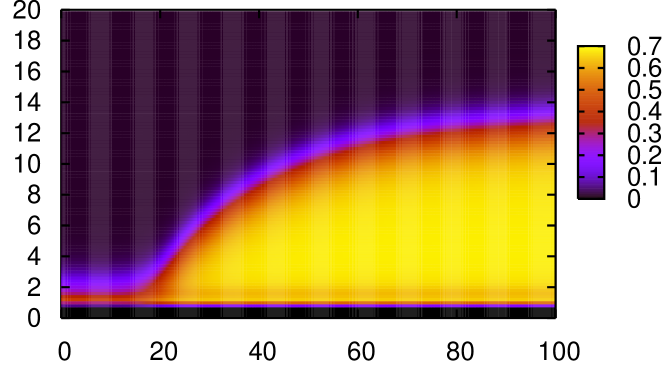
Figure 12: Equilibrium density profile between two equilibrium film thicknesses for the long-range wall potential $V_{\text{LJ}}$ given by equation (10c). The temperature is $T=0.7\,T_{\text{c}}$ and the chemical potential is $\mu=\mu_{\text{coex}}$. The wall parameters are $\beta_{\text{c}}\epsilon_{\text{w}}\approx 1.5$, $\sigma_{\text{w}}=1.25\,d$ and $z_{\text{w}}=0$. The shade values provided to the right of the figure correspond to the level values of $nd^{3}$.

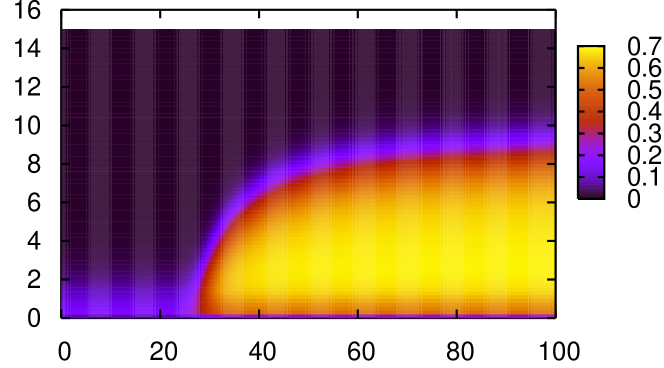
Figure 13: Equilibrium density profile between two equilibrium film thicknesses for the short-range wall potential $V_{\text{SR}}$ given by equation (10a). The temperature is $T=0.7\,T_{\text{c}}$ and the chemical potential is $\mu=\mu_{\text{coex}}$. The wall parameters are $\beta_{\text{c}}\epsilon_{\text{w}}=2.0$, $\sigma_{\text{w}}=1.25\,d$ and $z_{\text{w}}=0$. The shade values provided to the right of the figure correspond to the level values of $nd^{3}$.

IV.3 Contact angle

We now turn to the study of the density profile when $\mu=\mu_{\text{sat}}$ and the wall is attractive with a potential given by equation (10c). Recall from our discussion in § III.3 that up to $\mu_{\text{coex}}\rightarrow\mu^{-}_{\text{sat}}$ we can have a Maxwell construction with a thin film co-existing with an almost infinite thick film, while at $\mu=\mu_{\text{sat}}$ we loose the Maxwell construction and the thin film is the most stable state. Again, as in § IV.2, two different conditions are imposed on each side of the domain. The wall parameter $\epsilon_{\text{w}}$ is chosen so that a stable film of finite thickness can be sustained on the wall. According to figure 5, this is true for $V_{\text{LJ}}$ when $\beta_{\text{c}}\epsilon_{\text{w}}$ is at least in the range 0.8–1.4. The corresponding 1D density profile computed in § III will make up the boundary condition on the left side of the domain. On the right side, a thick film of arbitrary thickness $h_{\text{right}}$ and shape is imposed (unlike the equilibrium film to the left, to the right we do not have an equilibrium film). For simplicity the latter is taken to be a step function:

$$n_{\text{right}}(z)={}\begin{cases}n_{\text{liq}}\quad\text{if $z<z_{\text{w}}+h_{\text{right}}$}\\ n_{\text{gas}}\quad\text{if $z>z_{\text{w}}+h_{\text{right}}$}.\\ \end{cases}$$ (16)

An equilibrium density profile for an attractive wall obtained under these conditions is depicted in figure 14. The main feature is the presence of a well formed angle between the two phases. This is more evident in the current profiles than in the profiles obtained in § IV.2, quite likely because now the film profile on the right side of the domain is no longer an equilibrium one. Note also the liquid film present in front of the contact line area as the wall is attractive. Moreover, it is important to establish that the profile is not affected by the film thickness to the right. Indeed, as demonstrated in figure 15, the thickness of the film in the right side of the domain has little influence on the density profile since, for all values of $h_{\text{right}}$, the level curves are parallel to each other sufficiently far from the contact line.

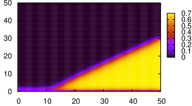
Figure 14: Equilibrium density profile for a fluid in contact with an attractive wall, whose potential is $V_{\text{LJ}}$ (equation (10c)). The temperature is $T=0.7\,T_{\text{c}}$, and the chemical potential is $\mu=\mu_{\text{sat}}$. The wall parameters are $\beta_{\text{c}}\epsilon_{\text{w}}=1.3$, $\sigma_{\text{w}}=1.25\,d$ and $z_{\text{w}}=0$. The contact angle is close to $37^{\circ}$.

Figure 15: Density level curves (corresponding to $n=(n_{\text{liq}}+n_{\text{gas}})/2$) for three different values of film thickness $h_{\text{right}}$ imposed on the right side of the domain: $h_{\text{right}}/d=18$ (right curve), $24$ and $30$ (left curve). In all cases, the same film is imposed on the left side of the domain. All parameters are identical to those of figure 14.

A cut in the density profile displayed in figure 14 far from the contact area and normal to the liquid-gas interface is shown in figure 16. A comparison with the profile in figure 2 reveals that the two are very close to each other: the interface sufficiently far from the contact line is simply the usual liquid-gas interface, i.e. with no wall present. In other words, away from the contact line, the interface shape is not affected by the wall and it is like having the usual liquid-gas interface there. However, a deviation from the liquid-gas interface occurs in the three-phase area where a small incurvation of the density profile towards the wall is observed. We shall return to this point shortly.

Figure 16: Liquid-gas interface (solid line) from Fig. 2 and cut in the density profile pictured in Fig. 14 normal to the liquid-gas interface (dotted line). The two profiles are very close to each other.

The surface tension of the interface is related to the grand potential $\Omega$ via

$$\sigma=\frac{\Omega-\Omega_{\text{bulk}}}{\mathcal{A}}$$ (17)

where $\Omega_{\text{bulk}}$ is the sum of the grand potentials of the two bulk phases and $\mathcal{A}$ is the area of the interface under consideration. Surface tensions for the planar wall/gas, wall/liquid and liquid/gas interfaces can be computed from the density profile constructed in figure 14. Simple analytical expressions can also be derived in the sharp interface limit for an infinite system and are given in Appendix A. From the surface tension values, one can calculate the contact angle $\theta$ from the Young equation,

$$\sigma_{\text{wg}}=\sigma_{\text{wl}}+\sigma_{\text{lg}}\cos\theta\text{,}$$ (18)

and contrast it with the one obtained by a direct geometric measurement in figure 17 using density level curves. We note that the choice of the specific level curve is not important since, as it has been demonstrate in figure 16, away from the contact line the interface shape is very close to the one corresponding to the liquid-gas interface without wall, and consequently two different level curves would yield the same geometric contact angle. Results for several values of $\epsilon_{w}$ are given in Table 1. A very good agreement is found between the two values of the contact angle. The main discrepancy between the two is quite likely caused by the error in the drawing of the dotted lines in figure 17. The computations in figure 17 also indicate that increasing the wall attraction decreases the contact angle (as expected).

$\beta_{\text{c}}\epsilon_{\text{w}}$	$\beta_{\text{c}}d^{2}\sigma_{\text{wg}}$	$\beta_{\text{c}}d^{2}\sigma_{\text{wl}}$	$\beta_{\text{c}}d^{2}\sigma_{\text{lg}}$	$\theta_{\text{num}}({}^{\circ})$	$\theta_{\text{mes}}({}^{\circ})$
$1.0$	$-0.0821$	$-0.253$	$0.503$	$70.2$	$70.8$
$1.1$	$-0.106$	$-0.360$	$0.503$	$59.7$	$60.7$
$1.2$	$-0.136$	$-0.470$	$0.503$	$48.4$	$49.5$
$1.3$	$-0.171$	$-0.582$	$0.503$	$35.2$	$36.6$

Table 1: Wall/gas ($\sigma_{\text{wg}}$), wall/liquid ($\sigma_{\text{wl}}$) and liquid/gas ($\sigma_{\text{lg}}$) surface tensions, and computed ($\theta_{\text{num}}$) and measured ($\theta_{\text{mes}}$) contact angles corresponding to figure 17.

Figure 17: Density level curves corresponding to $n=(n_{\text{liq}}+n_{\text{gas}})/2$ for several values of $\epsilon_{\text{w}}$. From right to left: $\beta_{\text{c}}\epsilon_{\text{w}}=1.0$, $\beta_{\text{c}}\epsilon_{\text{w}}=1.1$, $\beta_{\text{c}}\epsilon_{\text{w}}=1.2$ and $\beta_{\text{c}}\epsilon_{\text{w}}=1.3$. The contact angle in each case is measured by following the dotted lines. The wall potential is $V_{\text{LJ}}$, the temperature $T=0.7\,T_{\text{c}}$ and the chemical potential $\mu=\mu_{\text{sat}}$. The wall parameters are $\sigma_{\text{w}}=1.25\,d$ and $z_{\text{w}}=0$.

IV.4 Contact line

A close inspection of the contact line area in figure 17 reveals a deviation between the geometric profile suggested by Young’s equation and the one obtained from DFT close to the contact line where the interface seems to bend towards the wall and away from the dotted lines corresponding to Young’s equation. This feature appears to be in agreement with recent experiments by Seemann et al. (2005). The experiments are actually done for a two-layer composite wall, but when the top layer is thin, the interface close to the contact line appears to be similar to that shown in figure 17.

Level curves constructed with wall potentials $V_{\text{SR}}$ and $V_{\text{LR}}$ in equations (10a) and (10b), are given in figures 18 and 19, respectively. The bend is not present in the first case which suggests that it is mainly due to the long-range nature of the attraction of the wall potential. A parallel can be made with the conclusions of § IV.2 regarding the density shape in the transition area between the two films: as the contact angle goes to zero, the profiles in Fig. 18 seem to tend to the one in figure 13 giving rise to an abrupt transition between the two films while the ones in figure 19 seem to lead to the profile in figure 12 for which a smoother transition between the two films is observed. In contrast, no dramatic difference is observed between $V_{\text{LJ}}$ (figure 17) and $V_{\text{LR}}$ (figure 19) implying that the shape of the repulsive part of the wall potential is less critical.

Cuts in the contact line area normal to the wall are shown in figure 20 for the two potentials $V_{\text{SR}}$ and $V_{\text{LR}}$ in equations (10a) and (10b), respectively. We note that the density profiles are characterized by a small depression in the immediate vicinity of the wall ($x/d\approx 0.5$), although this feature disappears in the case of the short range wall potential $V_{\text{SR}}$ as we move away from the contact line towards the liquid. In contrast, it is present in the long range case even in the 1D case as shown in figure 3 for $z\approx 2d$.

Figure 18: Density level curves corresponding to $n=(n_{\text{liq}}+n_{\text{gas}})/2$ for wall potential $V_{\text{SR}}$ and several values of $\epsilon_{\text{w}}$. From right to left: $\beta_{\text{c}}\epsilon_{\text{w}}=1.4$, $\beta_{\text{c}}\epsilon_{\text{w}}=1.5$, $\beta_{\text{c}}\epsilon_{\text{w}}=1.6$, $\beta_{\text{c}}\epsilon_{\text{w}}=1.7$ and $\beta_{\text{c}}\epsilon_{\text{w}}=1.8$. The temperature is $T=0.7\,T_{\text{c}}$ and the chemical potential $\mu=\mu_{\text{sat}}$ while the wall parameters are $\sigma_{\text{w}}=1.25\,d$ and $z_{\text{w}}=0$.

Figure 19: Density level curves corresponding to $n=(n_{\text{liq}}+n_{\text{gas}})/2$ for wall potential $V_{\text{LR}}$ and several values of $\epsilon_{\text{w}}$. From right to left: $\beta_{\text{c}}\epsilon_{\text{w}}=1.7$, $\beta_{\text{c}}\epsilon_{\text{w}}=1.8$, $\beta_{\text{c}}\epsilon_{\text{w}}=1.9$, $\beta_{\text{c}}\epsilon_{\text{w}}=2.0$ and $\beta_{\text{c}}\epsilon_{\text{w}}=2.1$. The temperature is $T=0.7\,T_{\text{c}}$ and the chemical potential $\mu=\mu_{\text{sat}}$ while the wall parameters are $\sigma_{\text{w}}=1.25\,d$ and $z_{\text{w}}=0$.

Figure 20: Density profiles around the contact line area for the cases depicted in figure 18 ($\beta_{\text{c}}\epsilon_{\text{w}}=1.8$, solid lines) and in figure 19 ($\beta_{\text{c}}\epsilon_{\text{w}}=2.0$, dotted lines). Bottom/top curves correspond to the left/right of the contact line region in steps of 2 for $x/d$.

V Summary

We have examined the equilibrium of a fluid in contact with a solid substrate through a DFT theory based on a perturbation approach in which the interaction potential is split into a repulsive and an attractive part. This leads to three distinct parts in the expression for the free-energy functional, corresponding to repulsion, attraction and external potential associated with the presence of the solid boundary, respectively.

We first investigated the 1D case of a liquid film in contact with the substrate. For values of the chemical potential less than but close to its saturation value, a liquid film exists in contact with the wall, even though in the absence of the wall the gas is the preferred state. The presence of the film is due to the attractive part of the wall potential. For a given temperature, we have constructed bifurcation diagrams for the film thickness as a function of the chemical potential. Such diagrams are typically S-shaped curves with three branches. Comparison of the DFT theory with a gradient approach in which the integral DFT equation is approximated with a differential one reveals some significant qualitative differences. Any gradient approach is by definition a local one and as such it neglects the non-local features induced by the intermolecular forces acting on the fluid system.

The bifurcation diagrams reveal that there exists a special value of the chemical potential, which we referred to as “coexistence” value, in which a thin liquid film is equally stable with a thick one (“prewetting transition”). The interface that joins the two films is constructed with a fully 2D computation as now the translational invariance of the system in the direction parallel to the wall is broken. As the coexistence value tends to the saturation one, the thickness of the thick film tends to infinity. This then allows us to construct a liquid wedge in contact with the substrate and with a well-defined three-phase contact line. This wedge seems to persist for all distances from the substrate and hence it should eventually enter the macroscale. Comparison of the contact angle obtained from the DFT theory with a macroscopic model, such as the Young equation based on a mechanical force balance, shows good agreement a few molecular diameters far from the contact line. However, unlike the Young equation which requires information on macroscopic parameters, such as the surface tensions between the different phases, the DFT theory relies only on well-defined intermolecular parameters.

Of particular interest would be the extension of this approach to: (a) Spatially heterogeneous, chemical or topographical substrates. Such substrates have a significant effect on the wetting characteristics of the solid-liquid pair (e.g. Schwartz & Elley (1998), Gramlich et al. (2004), Quéré (2007), Savva & Kalliadasis (2009), Savva et al. (2010)); (b) The substantially more involved dynamic case. This would form the basis for the formulation of a dynamic contact angle theory from first principles without the need for any phenomenological parameters. We shall examine these problems in a future study.

VI Acknowledgements

We are grateful to Alexandr Malijevsky, Andreas Nold, Nikos Savva and Petr Yatsyshin for stimulating discussions and useful comments and suggestions. We acknowledge financial support from EPSRC Platform Grant No. EP/E046029.

Appendix A Expressions

A.1 Surface tensions

For a planar interface (i.e. the 1D case), analytical expressions for the surface tensions can be derived in the sharp interface limit for an infinite system. They read:

$$\sigma_{\text{lg}}=-\frac{1}{2}{(n_{\text{liq}}-n_{\text{gas}})}^{2}I$$ (19a)

$$\sigma_{\text{wg}}=-\frac{1}{2}n_{\text{gas}}^{2}I+n_{\text{gas}}\int_{0}^{+\infty}\text{d}zV(z)$$ (19b)

$$\sigma_{\text{wl}}=-\frac{1}{2}n_{\text{liq}}^{2}I+n_{\text{liq}}\int_{0}^{+\infty}\text{d}zV(z)$$ (19c)

where

$$I=\int_{-\infty}^{0}\text{d}z\int_{0}^{+\infty}\text{d}z^{\prime}\Phi_{\text{1d}}(z^{\prime}-z)\text{.}$$ (19d)

Such expressions are also applicable in the contact-angle case sufficiently far from the contact line, i.e. when the interface is planar.

In the following, we provide analytical expressions used both in the 1D and 2D computations.

A.2 Interaction potential

The perturbative part of the interaction potential between fluid molecules in the Barker-Henderson case is:

$$\phi_{\text{p}}(r)={}\begin{cases}\displaystyle 0\quad&\text{if $r<\sigma$}\\ \displaystyle 4\epsilon\left[{\left(\frac{\sigma}{r}\right)}^{12}-{\left(\frac{\sigma}{r}\right)}^{6}\right]\quad&\text{if $r>\sigma$}.\end{cases}$$ (20)

A.2.1 Derivation of $\Phi$

In the 1D case, $\Phi$, which enters the equation for the density, is defined as:

$$\Phi_{\text{1d}}(\beta)=\int\!\!\!\!\!\int_{-\infty}^{+\infty}\!\!\!\text{d}x\,\text{d}y\,\phi_{\text{p}}\!\left(\sqrt{x^{2}+y^{2}+\beta^{2}}\right).$$ (21)

Let us introduce ${\bar{\beta}}=\beta/\sigma$. Using Eq. (20), we obtain:

$$\Phi_{\text{1d}}={}\begin{cases}\displaystyle-2\pi\epsilon\sigma^{2}\frac{3}{5}\quad&\text{if $|{\bar{\beta}}|<1$}\\ \displaystyle 2\pi\epsilon\sigma^{2}\frac{1}{{\bar{\beta}}^{4}}\left(\frac{2}{5}\frac{1}{{\bar{\beta}}^{6}}-1\right)\quad&\text{if $|{\bar{\beta}}|>1$}.\end{cases}$$ (22)

In the 2D case $\Phi$ is defined as:

$$\Phi_{\text{2d}}(\beta)=\int_{-\infty}^{+\infty}\!\!\!\text{d}y\,\phi_{\text{p}}\left(\sqrt{y^{2}+\beta^{2}}\right)$$ (23)

For $|{\bar{\beta}}|<1$ we obtain:

$$\Phi_{\text{2d}}=8\epsilon\sigma \left[\frac{1}{{\bar{\beta}}^{11}}\left\{\frac{63}{256}\left(\frac{\pi}{2}-\arctan\left(\sqrt{\frac{1-{\bar{\beta}}^{2}}{{\bar{\beta}}^{2}}}\right)\right)\right.\right.$$

$$\qquad\left.{}-\sqrt{\frac{1-{\bar{\beta}}^{2}}{{\bar{\beta}}^{2}}}\frac{{\bar{\beta}}^{2}(128{\bar{\beta}}^{8}+144{\bar{\beta}}^{6}+168{\bar{\beta}}^{4}+210{\bar{\beta}}^{2}+315)}{1280}\right\}$$

$${}-\frac{1}{{\bar{\beta}}^{5}}\left\{\frac{3}{8}\left(\frac{\pi}{2}-\arctan\left(\sqrt{\frac{1-{\bar{\beta}}^{2}}{{\bar{\beta}}^{2}}}\right)\right)\left.{}-\sqrt{\frac{1-{\bar{\beta}}^{2}}{{\bar{\beta}}^{2}}}\frac{{\bar{\beta}}^{2}(2{\bar{\beta}}^{2}+3)}{8}\right\}\right],$$ (24)

and for $|{\bar{\beta}}|>1$:

$$\Phi_{\text{2d}}=\frac{3}{2}\epsilon\pi\sigma\frac{1}{{\bar{\beta}}^{5}}\left[\frac{21}{32}\frac{1}{{\bar{\beta}}^{6}}-1\right].$$ (25)

A.3 External potential

The Lennard-Jones expression of the wall potential can be obtained by considering that the wall is made of particles which interact with the fluid molecules via a pair potential of the Lennard-Jones form:

$$v(r)=4\epsilon^{\prime}_{\text{w}}\left({\left(\frac{\sigma_{\text{w}}}{r}\right)}^{12}-{\left(\frac{\sigma_{\text{w}}}{r}\right)}^{6}\right)$$ (26)

where $r$ is the distance between a wall particle and a fluid particle.

Let us consider the case of a planar wall. Our coordinate system has the three unit vectors $(\mathbf{i},\mathbf{j},\mathbf{k})$ with $\mathbf{k}$ an outward unit vector normal to the wall. The wall is described as a continuous medium and the wall particles density, denoted by $n_{\text{w}}$, is taken uniform. The the edge of the wall, which is in direct contact with the fluid, is located at $z^{\prime}_{w}$ so that $n_{\text{w}}=0$ if $z>z^{\prime}_{\text{w}}$. The overall potential exerted by the wall at position $(x_{0},y_{0},z_{0})$ in the fluid domain ($z_{0}>z^{\prime}_{\text{w}}$) is,

$$V(x_{0},y_{0},z_{0})=\int_{z<z^{\prime}_{\text{w}}}\text{d}\tau\,n_{\text{w}}v(r)$$ (27)

where $n_{\text{w}}$ denotes the wall particles density and is assumed constant. As the wall is invariant in the $(\mathbf{i},\mathbf{j}$) directions, $V$ only depends on $z_{0}$. Using cylindrical coordinates, we obtain,

$$V(z_{0})=\int_{0}^{+\infty}\!\!\!\!\!R\text{d}R\int_{0}^{2\pi}\!\!\!\!\!\text{d}\theta\int_{-\infty}^{z^{\prime}_{\text{w}}}\!\!\!\!\!\text{d}z\,n_{\text{w}}\,v\!\left(\sqrt{R^{2}+{(z_{0}-z)}^{2}}\right)$$ (28)

which for $z_{0}>z^{\prime}_{\text{w}}$ yields:

$$V(z_{0})=4\pi\epsilon^{\prime}_{\text{w}}n_{\text{w}}\sigma_{\text{w}}^{3}{\left(\frac{\sigma_{\text{w}}}{z_{0}-z^{\prime}_{\text{w}}}\right)}^{3}\left[\frac{2}{15}{\left(\frac{\sigma_{\text{w}}}{z_{0}-z^{\prime}_{\text{w}}}\right)}^{6}-1\right].$$ (29)

Appendix B Numerical method

B.1 1D case

The equation to solve reads:

$$\mu_{\text{r}}[n](z)+\int_{-\infty}^{+\infty}\!\text{d}z^{\prime}n(z^{\prime})\Phi_{\text{1d}}(z^{\prime}-z)+V(z)=\mu$$ (30)

for $n(z)$ in the domain $\mathcal{D}_{\text{1d}}=]z_{0},z_{N_{z}}[$ with conditions $n=n_{0}$ for $z\leq z_{0}$ and $n=n_{N_{z}}$ for $z\geq z_{N_{z}}$. In the presence of the wall we assume $z_{0}\geq z_{\text{w}}$ (or $z_{0}\geq z^{\prime}_{\text{w}}$). We introduce a uniform mesh: $z_{i}=z_{0}+\Delta z\,i$, $i=0...N_{z}$. The integral is computed by using a trapezoidal rule in the interval $[z_{0},z_{N_{z}}]$ while analytical expressions are utilized outside this interval, obtained by using (22) and the fact that the density there is constant ($=n_{\text{l,g}}$). We then obtain a system of $N_{z}-1$ nonlinear equations for the unknowns $n_{i}=n(z_{i})$, $i=1...N_{z}-1$, which are solved by using a Newton scheme. In order to speed up the scheme, the off-diagonal elements of the Jacobian matrix are neglected as they are smaller compared to the diagonal ones (this is especially so far from the diagonal). The Jacobian matrix can then be inverted analytically in each iteration step.

B.2 2D case

The equation to solve reads:

$$\mu_{\text{r}}[n](z)+\int\!\!\!\!\!\int_{-\infty}^{+\infty}\!\!\!\!\text{d}x^{\prime}\text{d}z^{\prime}n(x^{\prime},z^{\prime})\Phi_{\text{2d}}\!\left(\sqrt{\scriptstyle{(x^{\prime}-x)}^{2}+{(z^{\prime}-z)}^{2}}\right)+V(x,z)=\mu$$ (31)

for $(x,z)\in\mathcal{D}_{\text{2d}}$ where $\mathcal{D}_{\text{2d}}=]x_{0},x_{N_{x}}[\times]z_{0},z_{N_{z}}[$. In the presence of a wall, $z_{0}\geq z_{\text{w}}$ (or $z_{0}\geq z^{\prime}_{\text{w}}$). The conditions outside this domain are $n(x,z)=n_{\text{l}}(z)$ if $x\leq x_{0}$, $n(x,z)=n_{\text{r}}(z)$ if $x\geq x_{N_{x}}$, $n(x,z)=n_{b}$ if $z\leq z_{0}$ and $n(x,z)=n_{t}$ if $z\geq z_{N_{z}}$ The functions $n_{\text{l}}$ and $n_{\text{r}}$ are such that $n_{\text{l}}(z)=n_{b}$ and $n_{\text{r}}(z)=n_{b}$ if $z\leq z_{0}$, and $n_{\text{l}}(z)=n_{t}$ and $n_{\text{r}}(z)=n_{t}$ if $z\geq z_{N_{z}}$. This choice of conditions for $x\leq x_{0}$ and $x\geq x_{N_{x}}$ allows us to examine, for example, the case of a fluid in contact with two liquid films of different thicknesses, one on each side.

A uniform mesh is used to compute $n(x,z)$: $x_{j}=x_{0}+\Delta x\,j$, $j=0...N_{x}$, and $z_{i}=z_{0}+\Delta z\,i$, $i=0...N_{z}$. Equation (31) is solved for $n_{ji}=n(x_{j},z_{i})$, $j=1...N_{x}-1$ and $i=1...N_{z}-1$. The integral appearing in the equation is computed by dividing the integration domain into three parts: $\mathcal{D}_{\text{2d}}$, $\mathcal{D}^{\prime}_{\text{2d}}-\mathcal{D}_{\text{2d}}$ and $]-\infty,+\infty[\times]-\infty,+\infty[-\mathcal{D}^{\prime}_{\text{2d}}$. The domain $\mathcal{D}^{\prime}_{\text{2d}}$ is defined as $\mathcal{D}^{\prime}_{\text{2d}}=]x^{\prime}_{0},x^{\prime}_{N_{x}}[\times]z^{\prime}_{0},z^{\prime}_{N_{z}}[$, where $x^{\prime}_{0}=x_{0}-\sigma$, $x^{\prime}_{N_{x}}=x_{N_{x}}+\sigma$, $z^{\prime}_{0}=z_{0}-\sigma$ and $z^{\prime}_{N_{z}}=z_{N_{z}}+\sigma$. Outside $\mathcal{D}^{\prime}_{\text{2d}}$, Eq.(25) is used for any $n_{ji}\in\mathcal{D}_{\text{2d}}$ and analytical expressions can be derived for the integral when $|x^{\prime},z^{\prime}|\rightarrow\infty$ where the density is constant ($=n_{\text{l,g}}$). In $\mathcal{D}^{\prime}_{\text{2d}}-\mathcal{D}_{\text{2d}}$, the integral is computed numerically by using either Eq. (24) or Eq. (25) once for all at the start of a run. In $\mathcal{D}_{\text{2d}}$, the integral has to be carried out numerically at each iteration.

The discretization of Eq. (31) leads to a set of $(N_{x}-1)\times(N_{z}-1)$ nonlinear equations for the $(N_{x}-1)\times(N_{z}-1)$ unknowns $n_{ji}$. It is solved by using a Newton scheme. To speed up the computations, the Jacobian is made sparse by neglecting contributions when $|\mathbf{r}_{1}-\mathbf{r}_{2}|$, where $\mathbf{r}_{1,2}$ the positions of two particles, is larger than a few molecular diameters: the non-diagonal terms of the Jacobian which involve $\Phi_{\text{2d}}(\mathbf{r}_{1}-\mathbf{r}_{2})$ (for the diagonal terms $\mathbf{r}_{1}-\mathbf{r}_{2}={\bf 0}$) are getting small as we move further from the diagonal since $|\mathbf{r}_{1}-\mathbf{r}_{2}|$ increases so that $\Phi_{\text{2d}}$ decreases. By doing so, more iterations are needed for convergence but each one is considerably faster than inverting the full Jacobian. Finally, at each iteration step, we have to solve a linear system involving a sparse matrix. This stage is performed with a Gauss-Siedel method.

References

- Argaman & Makov (2000) Argaman, N. & Makov, G. 2000 Density functional theory: An introduction. Am. J. Phys. 68, 69–79.
- Barker & Henderson (1967) Barker, J. A. & Henderson, D. 1967 Perturbation theory and equation of state for fluids. II. a successful theory of liquids. J. Chem. Phys. 47, 4714.
- Berim & Ruckenstein (2008a) Berim, G. O. & Ruckenstein, E. 2008a Microscopic calculation of the sticking force for nanodrops on an inclined surface. J. Chem. Phys. 129, 114709.
- Berim & Ruckenstein (2008b) Berim, G. O. & Ruckenstein, E. 2008b Nanodrop on a nanorough solid surface: Density functional theory considerations. J. Chem. Phys. 129, 014798.
- Berim & Ruckenstein (2009) Berim, G. O. & Ruckenstein, E. 2009 Simple expression for the dependence of the nanodrop contact angle on liquid-solid interactions and temperature. J. Chem. Phys. 130, 044709.
- Bonn et al. (2009) Bonn, D., Eggers, J., Indekeu, J., Meunier, J. & Rolley, E. 2009 Wetting and spreading. Rev. Mod. Phys. 81, 739.
- E. B. Dussan & Davis (1974) E. B. Dussan, V. & Davis, S. H. 1974 On the motion of a fluid-fluid interface along a solid surface. J. Fluid. Mech. 65, 71–95.
- Evans (1979) Evans, R. 1979 The nature of the liquid-vapour interface and other topics in the statistical mechanics of non-uniform, classical fluids. Adv. Phys. 28, 143.
- de Gennes (1985) de Gennes, P.-G. 1985 Wetting: Statics and Dynamics. Rev. Mod. Phys. 57, 827.
- Gramlich et al. (2004) Gramlich, C., Mazouchi, A. & Homsy, G. 2004 Time-dependent free surface stokes flow with a moving contact line. II. Flow over wedges and trenches. Phys. Fluids 16, 1660–1667.
- Huh & Scriven (1971) Huh, C. & Scriven, L. E. 1971 Hydrodynamic model of steady movement of a solid/liquid/fluid contact line. J. Colloid Interface Sci. 35, 85–101.
- Landau & Lifshitz (1980) Landau, L. D. & Lifshitz, E. M. 1980 Statistical Physics, Part I. Pergamon Press.
- Miranville (2003) Miranville, A. 2003 Generalized cahn-hiliiard equations based on a microforce balance. J. Appl. Math. 4, 165–185.
- Moffat (1963) Moffat, H. K. 1963 Viscous and resistive eddies near a sharp corner. J. Fluid. Mech. 18, 1–18.
- Pismen (2002) Pismen, L. M. 2002 Mesoscopic hydrodynamics of contact line motion. Colloid Surf. A 206, 11.
- Plischke & Bergersen (2006) Plischke, M. & Bergersen, B. 2006 Equilibrium Statistical Physics. World Scientific.
- Quéré (2007) Quéré, D. 2007 Three-phase capillarity. In Thin Films of Soft Matter (ed. S. Kalliadasis & U. Thiele), pp. 115–136. Springer-Wien, NY.
- Rosenfeld (1989) Rosenfeld, Y. 1989 Free-energy model for the inhomogeneous hard-sphere fluid mixture and density-functional theory of freezing. Phys. Rev. Lett. 63, 980.
- Savva & Kalliadasis (2009) Savva, N. & Kalliadasis, S. 2009 Two-dimensional droplet spreading over topographical substrates. Phys. Fluids 21, 092192.
- Savva et al. (2010) Savva, N., Kalliadasis, S. & Pavliotis, G. 2010 Two-dimensional droplet spreading over random topographical substrates. Phys. Rev. Lett. 104, 084501.
- Schwartz & Elley (1998) Schwartz, L. & Elley, R. 1998 Simulation of droplet motion on low-energy and heterogeneous surfaces. J. Colloid Interface Sci. 202, 173–188.
- Seemann et al. (2005) Seemann, R., Herminghaus, S., Neto, C., Schlagowski, S., Podzimek, D., Konrad, R., Mantz, H. & Jacobs, K. 2005 Dynamics and structure formation in thin polymer melt films. J. Phys. Condens. Matter 17, S267–S290.
- Tarazona (1985) Tarazona, P. 1985 Free-energy density functional for hard spheres. Phys. Rev. A 31, 2672–2679.
- Teletzke et al. (1982) Teletzke, G. F., Scriven, L. E. & Davis, H. T. 1982 Gradient theory of wetting transitions. J. Colloid Interface Sci. 87, 550–571.
- Weeks et al. (1971) Weeks, J. D., Chandler, D. & Andersen, H. C. 1971 Role of repulsive forces in determining the equilibrium structure of simple liquids. J. Chem. Phys. 54, 5237.