Multiple scattering of light in superdiffusive media

Abstract

Light transport in superdiffusive media of finite size is studied theoretically. The intensity Green’s function for a slab geometry is found by discretizing the fractional diffusion equation and employing the eigenfunction expansion method. Truncated step length distributions and complex boundary conditions are considered. The profile of a coherent backscattering cone is calculated in the superdiffusion approximation.

Light transport in disordered media is characterized by a multiple scattering process engendered by random fluctuations of the refractive index in space and described perturbatively by expanding the field in powers of the scattering potential akkermansbook . Important quantities such as the angular distribution of backscattered and transmitted intensity can be calculated within a diffusion approximation and the Green’s function of the diffusive equation, or diffusion propagator, be used to describe fundamental interference effects like speckles and weak localization akkermansbook . The diffusive picture has its roots in the concept of Brownian motion, where random walkers perform independent steps of variable length, each with finite mean and variance. By virtue of the central limit theorem, the step length distribution after a large number of steps approaches a Gaussian distribution irrespectively of the microscopic transport mechanism. This rule, however, breaks down when the probability to perform arbitrary long steps is non-vanishing. In this case, the limiting distribution becomes a so-called $\alpha$-stable Lévy distribution levyoriginal and is characteristically heavy-tailed. Such random walks, first studied by Mandelbrot in the framework of transport on fractals mandelbrotfractal , are known as Lévy flights if steps of arbitrary length can be performed in a unit time and Lévy walks if performed at a finite velocity sokolovLW . As transport is dominated by a few huge steps, the resulting average distance explored by a walker increases faster with time than expected for standard diffusion. This type of anomalous transport is called superdiffusion anotrans and has been found to be ubiquitous in nature ubiquity . Superdiffusion of light has recently been observed in heterogeneous dielectric materials  WiersmaNature2008 and in hot atomic vapors kaiserlevyatom . On the theoretical level, superdiffusion has been modelled by employing the subordinator method sokolowsubordination and by generalizing the diffusion equation to fractional order derivatives yanovskyfractionaldiffusion . Previous works have evidenced the peculiar statistical properties of Lévy motions Chechkin2003 ; Koren2007 and shown that several features of real experiments, such as properly defined boundary conditions, are nontrivial to implement Chechkin2003 , making the description of observable quantities nearly impossible.

In this Letter, we develop a theoretical framework for multiple light scattering in superdiffusive media. Our approach, which relies on the semi-analytical solution of the fractional diffusion equation, allows to study the steady-state transport properties of superdiffusive media while taking into account the intrinsic finite size of actual materials and makes it possible to treat interference effects, notably coherent backscattering, in the “superdiffusion approximation”. In particular, we calculate the intensity Green’s function in the superdiffusive regime for various values of the $\alpha$ coefficient and show that arbitrary boundary conditions and truncations in the step length distribution can be implemented.

From the microscopic point of view, the disorder averaged intensity $I$ observed at a point $\mathbf{R}$ outside a multiple scattering medium can be written as

$$\begin{split}I(\mathbf{R})=&\int d\mathbf{r}_{1}d\,\mathbf{r}_{2}\,d\mathbf{r}_{3}\,d\mathbf{r}_{4}\,\phi(\mathbf{r}_{1})\,\phi^{\star}(\mathbf{r}_{2})\cdot\\ &\cdot f\left(\mathbf{r}_{1},\mathbf{r}_{2},\mathbf{r}_{3},\mathbf{r}_{4}\right)\,G(\mathbf{r}_{3},\mathbf{R})\,G^{\star}(\mathbf{R},\mathbf{r}_{4})\end{split}$$ (1)

where $\phi$ is the coherent (i.e. unscattered) propagator for the amplitude from outside the sample to the first scattering event, $G$ is the averaged propagator for the amplitude from the last scattering event to the point of observation $\mathbf{R}$ (i.e. the solution to the Dyson equation) and $f\left(\mathbf{r}_{1},\mathbf{r}_{2},\mathbf{r}_{3},\mathbf{r}_{4}\right)$ is the four-vertex propagator that contains all information about transport. When recurrent scattering is neglected, only two two-vertex terms contribute to $f$: the ladder term, which describes the incoherent transport, and the most-crossed term, which leads to the coherent backscattering cone cbs . More complicated combinations of these two terms can also be used to describe speckle correlations and intensity fluctuations leespecklecorrelations .

When the step length distribution $p(\ell)$ decays fast enough, the diffusion approximation holds and the propagator for the incoherent intensity transport satisfies the standard diffusion equation akkermansbook . On the other hand, for Lévy flights, the step length distribution exhibits a power-law tail of the form $p(\ell)\sim\ell^{-\left(\alpha+1\right)}$ with $0<\alpha\leq 2$, and the macroscopic motion is described by the diffusion-like equation anotrans :

$$\partial_{t}C\left(\mathbf{r},t\right)=D_{\alpha}\nabla^{\alpha}C\left(\mathbf{r},t\right)$$ (2)

where $\nabla^{\alpha}$ is the symmetric Riesz fractional derivative with respect to spatial coordinates and $D_{\alpha}$ is a generalization of the diffusion constant.

In the normal diffusive case, finite-size effects and internal reflection at the boundaries are handled by imposing that the propagator goes to zero at a distance from the physical boundaries called the extrapolation length weitzinternalreflections . This is possible because the Laplacian operator is local in space and thus, the presence of boundaries does not change the form of the propagator itself. On the other hand, the fractional Laplacian in Eq. 2 is non-local and, as such, the superdiffusive propagator is very sensitive to the nature of the boundaries. In fact, this propagator in non-infinite media is known only in a few particular cases reflectingboundarylevy . The description of superdiffusive transport in finite-size media therefore requires to determine the form of the propagator for arbitrary step length distributions and boundary conditions.

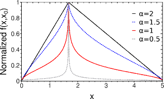
Figure 1: Normalized Green’s function $f\left(x,x_{0}\right)$ for a slab with $L=5$, $x_{0}=L/3$, $M=300$, $D_{\alpha}=1$ and absorbing boundaries, computed for various values of $\alpha$.

The problem of the non-locality of the fractional Laplacian can be circumvented by discretizing the fractional Laplacian podlubnydiscretefractional , i.e. by replacing the continuous time random walk by discrete hops on a lattice and $\nabla^{\alpha}$ by an $M\times M$ matrix, which, when applied to the vector representing our function $C$, converges to the continuum operator when $M$ goes to infinity. Let us consider a 1D system where space and time are discretized (the generalization to the 3D case will be presented later in this Letter) and define $\omega_{\left|i-j\right|}$ as the probability to perform a jump from site $i$ to site $j$. The macroscopic transport is expected to be described by Eq. 2 when the time and space discretizations are fine enough. Concurrently, the microscopic redistribution process that occurs at each time interval can be written as $C_{j}(t_{n+1})=\sum_{i}\omega_{\left|i-j\right|}C_{j}(t_{n})$ such that mainardidiscretization :

$$\frac{C_{j}(t_{n+1})-C_{j}(t_{n})}{\tau}=\frac{1}{\tau}\sum_{i=1}^{M}\left(\omega_{\left|i-j\right|}-\delta_{i,j}\right)C_{j}(t_{n}),$$ (3)

where $\delta_{i,j}$ is the Kronecker delta.

In the limit $\tau\rightarrow 0$, the left- and right-hand sides of this equation represent $\partial_{t}C_{j}(t)$ and $D_{\alpha}\nabla^{\alpha}C_{j}(t)$, respectively. Any microscopic redistribution property, provided that it leads to superdiffusion, can therefore be used to write a discretized version of the fractional Laplacian. In particular, if $\Omega$ is the matrix of transition probabilities, we have:

$$D_{\alpha}\nabla^{\alpha}\sim\lim_{\tau\rightarrow 0}\frac{1}{\tau}\left(\Omega-\mathbbm{1}\right).$$ (4)

The convergence properties of this limit depend on the particular choice of the transition probabilities. The most natural choice, $\omega_{\left|i-j\right|}\propto\left|i-j\right|^{-\left(\alpha+1\right)}$, is known to suffer from a poor convergence, especially when $\alpha\rightarrow 2$ Buldyrev1992 . A much faster convergence has been demonstrated zoiafractional using a direct discretization of the fractional Laplacian, leading to podlubnydiscretefractional :

$$\Omega_{i,j}=\frac{1}{h^{\alpha}}\frac{\Gamma\left(-\frac{\alpha}{2}+\left|i-j\right|\right)\Gamma\left(\alpha+1\right)}{\pi\Gamma\left(1+\frac{\alpha}{2}+\left|i-j\right|\right)},$$ (5)

where $h$ is the distance between two consecutive nodes on the lattice and $\Gamma$ is the Euler gamma function. In this framework, setting $\omega_{\left|i-j\right|}=0$ when $j$ is outside a given interval $\left[0,L\right]$ corresponds to the situation in which walkers stepping out of the interval cannot ever re-enter it. Thus, reducing the infinite size matrix $\Omega$ to a $M\times M$ matrix comes to imposing a finite size with absorbing boundary conditions to the system zoiafractional .

A physical model for superdiffusion in real systems should rely on Lévy walks rather than on Lévy flights since all jumps are bound to have a finite velocity. The resulting spatiotemporal coupling sokolovLW is known to make the description of Lévy walks difficult to handle analytically meerchaertlevywalk as opposed to Lévy flights, essentially described by Eq. 2. This coupling, however, becomes irrelevant in the steady-state regime since the amount of time required to perform a jump plays no role. The intensity Green’s function in a 1D superdiffusive medium for a continuous point source at $x_{0}$ is then given by the following time-independent fractional differential equation:

$$D_{\alpha}\nabla^{\alpha}f\left(x,x_{0}\right)=-\delta(x-x_{0}).$$ (6)

Note that $f\left(x,x_{0}\right)$ is the two-vertex propagator appearing in Eq. 1 in the superdiffusion approximation.

A complete description of the operator $\nabla^{\alpha}$ is provided by the eigenfunctions $\psi_{i}$ and eigenvalues $\lambda_{i}$ of the matrix $\Omega-\mathbbm{1}$, with $h=L/M$. Then, $f$ can be expanded in terms of the eigenfunctions $\psi_{i}$ as a linear combination $f\left(x\right)=\sum_{i}a_{i}\psi_{i}$, where $a_{i}$’s are the coefficients to be determined. By substituting the above expressions in Eq. 6 and considering that $\psi_{j}(x)\psi_{i}(x)=\delta_{i,j}$, we obtain $a_{i}=-\psi_{i}(x_{0})\left(D_{\alpha}\lambda_{i}\right)^{-1}$, yielding the Green’s function of a 1D superdiffusive motion of exponent $\alpha$:

$$f\left(x,x_{0}\right)=-\sum_{i=1}^{M}\frac{\psi_{i}\left(x\right)\psi_{i}\left(x_{0}\right)}{D_{\alpha}\lambda_{i}}.$$ (7)

Figure 1 shows the normalized Green’s function $f$ for different values of $\alpha$. For $\alpha=2$ we recover the familiar triangular shape typical of the diffusive regime while the Green’s function becomes more and more cusped when $\alpha$ decreases.

The microscopic transport mechanism of light in real systems is subject to additional and more complex features, including a truncation in the step length distribution and partially or totally reflecting boundaries. Those can be taken into account through Eq. 4 by modifying the transition probabilities $\omega_{\left|i-j\right|}$ in the medium. Truncated Lévy step distributions Mantegna1994 , which are unavoidable in finite-size systems WiersmaNature2008 , can be implemented by setting to zero all transition matrix elements where $\left|i-j\right|\geq l_{\text{max}}$ and renormalizing $\Omega$ so that $\sum_{j}\omega_{\left|i-j\right|}=1\,\forall\,i$ before introducing the boundaries. Figure 2a shows how the normalized Green’s function at constant $\alpha$ changes with the truncation length. While when $l_{\text{max}}\simeq L$ there is only a minor correction to the shape of the Green’s function, $f\left(x,x_{0}\right)$ becomes very similar to the diffusive one when $l_{\text{max}}\ll L$.

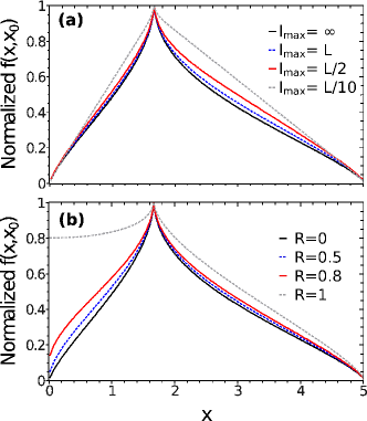
Figure 2: Normalized Green’s function $f\left(x,x_{0}\right)$ for a slab with $\alpha=1.5$, $L=5$, $x_{0}=L/3$, $M=300$ and $D_{\alpha}=1$, computed for various values of (a) $l_{\text{max}}$ and (b) the reflectance $R$ on the left boundary.

Partially reflecting boundaries are also expected to change the shape of the propagator. They can be implemented by considering that walkers reaching a boundary of the superdiffusive media have a probability $R$ to be reflected. In the case where the left boundary has reflectance $R$ while the right one is totally absorbing, partial reflection is enforced by mapping all matrix elements corresponding to $j<0$ onto their mirror images, yielding $\Omega_{i,j}=\omega_{\left|i-j\right|}+R\,\omega_{i+j+1}-\delta_{i,j}$. The case of both partially reflecting boundaries are conceptually analogous albeit a bit more involved due to the fact that one has to consider the possibility of performing very long steps that might bounce forth and back a large number of times. Figure 2b shows the normalized Green’s function for different values of the reflectance $R$ of the left boundary. Note that when $R=1$ the gradient of $f\left(x,x_{0}\right)$ on the left boundary goes to zero as expected reflectingboundarylevy .

Up to now, we have considered the 1D case of superdiffusive transport in finite media. Our approach can easily be extended to higher dimensions in the case of a slab geometry. Orienting the slab such that its interface is normal to the $x$-axis, the system becomes translationally invariant in both $y$- and $z$-directions. The 3D counterpart of Eq. 6 can then be written in terms of the Fourier transform of $f(\mathbf{r},\mathbf{r}_{0})$ in the $yz$-plane as:

$$D_{\alpha}\left(\nabla^{\alpha}_{x}-k_{\perp}^{\alpha}\right)f\left(x,x_{0},\mathbf{k}_{\perp}\right)=-\delta(x-x_{0}).$$ (8)

Applying to Eq. 8 the approach used to find Eq. 7, we find:

$$f(x,x_{0},\mathbf{k}_{\perp})=-\sum_{i=1}^{M}\frac{\psi_{i}(x_{0})\psi_{i}(x)}{D_{\alpha}\left(\lambda_{i}-k_{\perp}^{\alpha}\right)},$$ (9)

where $k_{\perp}=|\mathbf{k}_{\perp}|$. The 3D Green’s function of the superdiffusive medium can be obtained at this point by performing an inverse Fourier transform of Eq. 9. The full intensity distribution in the system (including the transmission profile WiersmaNature2008 ) can be obtained upon integration over a suitable source. As shown below, Eq. 9 can also be used to compute the shape of the coherent backscattering cone in the superdiffusion approximation.

In the multiple scattering regime, interferences can play a major role in determining the transport properties of the medium. In particular, in the exact backscattered direction, the interference coming from counterpropagating paths is always constructive as long as the system is reciprocal akkermansbook . This leads to a narrow cone of enhanced albedo in reflection known as the coherent backscattering cone. If reciprocity is not broken, the peak of the enhanced albedo is exactly twice the common incoherent reflection and presents a triangular cusp on the top wiersmacbs while its exact shape depends on transport in the medium. As a rule of thumb, long paths contribute to the formation of the cusp and short ones to the tails of the cone. Since in a superdiffusive regime there is no a priori reason for reciprocity to break down, we expect longer paths to contribute more than in standard diffusion and thus, expect a sharper peak.

The coherent component of the albedo $A$ can be calculated starting from Eq. 1 by setting $\mathbf{r}_{1}=\mathbf{r}_{4}$ and $\mathbf{r}_{2}=\mathbf{r}_{3}$  akkermansbook . Considering a planewave at normal incidence on the slab interface, using the Fraunhofer approximation for the Green’s functions and assuming that the step distribution follows a power-law, we can write:

$$\begin{split}&\phi(\mathbf{r}_{1})=x_{1}^{-\left(\alpha+1\right)/2}\;e^{i\mathbf{k}_{\text{i}}\cdot\mathbf{r}_{1}}\\ &G(\mathbf{r}_{2},R)=\left(\frac{x_{2}}{\cos\theta}\right)^{-\left(\alpha+1\right)/2}\;e^{-i\mathbf{k}_{\text{e}}\cdot\mathbf{r}_{2}}\;\frac{e^{ikR}}{4\pi R}\end{split}$$

and similarly for $\phi^{\star}(\mathbf{r}_{2})$ and $G^{\star}(R,\mathbf{r}_{1})$, where $\theta$ is the angle with respect to the normal of the slab, $\mathbf{k}_{\text{i}}$ and $\mathbf{k}_{\text{e}}$ the wavevectors of the incident and emergent planewaves respectively, and $\mathbf{k}_{\perp}=(\mathbf{k}_{i}+\mathbf{k}_{e})_{\perp}$. After substitution in Eq. 1 and Fourier transform, we obtain:

$$A\propto\iint_{0}^{L}dx_{1}dx_{2}\;\left(\frac{x_{1}x_{2}}{\cos\theta}\right)^{-\left(\alpha+1\right)}f(x_{1},x_{2},\mathbf{k}_{\perp}).$$ (10)

Using the discretized approximation in Eq. 9 for the propagator $f(x_{1},x_{2},\mathbf{k}_{\perp})$, we find the following expression for the coherent albedo from a superdiffusive slab:

$$A\propto-\sum_{x_{1},x_{2}}\left(\frac{x_{1}x_{2}}{\cos\theta}\right)^{-\left(\alpha+1\right)}\sum_{i=1}^{M}\frac{\psi_{i}(x_{1})\psi_{i}(x_{2})}{D_{\alpha}\left(\lambda_{i}-\left|k\sin{\theta}\right|^{\alpha}\right)}.$$ (11)

Figure 3 shows the normalized profile of the coherent backscattering cone as a function of $\alpha$. When $\alpha$ is decreased the amount of light transmitted through the sample is increased (in the superdiffusive regime $T\propto L^{-\alpha/2}$ Buldyrev1992 ) yet, at the same time, long steps become increasingly important, thereby making the profile more cusped. We note that a similar effect has been predicted for enhanced backscattering in fractal media akkermansfractal . Note also that since all calculations are done considering a finite thickness, part of the light is lost by transmission through the system, and thus, the top of the cone for $\alpha=2$ appears rounded akkermansbook .

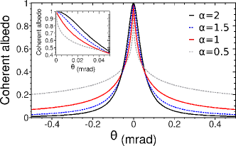
Figure 3: Normalized coherent albedo for a slab with $L=5$, $M=300$ and $D_{\alpha}=1$, computed for various values of $\alpha$. When $\alpha$ is decreased the contribution of long paths to the backscattering cone is larger leading to a sharper cusp and to tails that fall down more slowly (but still go to zero for $\theta=\pm\pi/4$). A zoomed view of the top of the curves is shown in the inset.

In conclusion, we obtained a semi-analytical formulation for the intensity Green’s funtion of multiple scattered light in the superdiffusive regime applying the eigenfunction expansion method to the discretized version of the steady-state fractional diffusion equation. This approach makes it possible to describe the behavior of many observable properties of superdiffusive media of finite size with complex boundary conditions (absorbing, partially reflecting, reflecting) as well as truncated step distributions. It also allows for the calculation of fundamental interference effects, such as the coherent backscattering cone, in the superdiffusion approximation.

- (1) E. Akkermans and G. Montambaux, Mesoscopic Physics of Electrons and Photons (Cambridge University Press, 2007).
- (2) P. Lévy, Théorie de l’addition des variables aléatoires (Gauthier-Villars, 1937).
- (3) B. Mandelbrot, The Fractal Geometry of Nature (V.H. Freeman & co., 1977).
- (4) I. M. Sokolov and R. Metzler, Phys. Rev. E 67, 010101(R) (2003).
- (5) R. Klages, G. Radons and I. M. Sokolov, Anomalous Transport (Wiley-VCH, 2008); R. Metzler and J. Klafter, Phys. Rep. 339, 1 (2000).
- (6) C. Tsallis et al., Phys. Rev. Lett. 75, 3589 (1995); A. Pekalski and K. Sznajd-Weron, Anomalous Diffusion: From Basics to Applications (Springer-Verlag Telos, 1999).
- (7) P. Barthelemy, J. Bertolotti and D. S. Wiersma, Nature 453, 495 (2008).
- (8) N. Mercadier et al., Nature Phys. 5, 602 (2009).
- (9) I. M. Sokolov, Phys. Rev. E 63, 011104 (2000).
- (10) V. V. Yanovsky et al., Physica A 282, 13 (2000).
- (11) A. V. Chechkin et al., J. Phys. A: Math. Gen. 36, L537 (2003).
- (12) T. Koren et al., Phys. Rev. Lett. 99, 160602 (2007).
- (13) Y. Kuga and A. Ishimaru, J. Opt. Soc. Am. A 1, 831 (1984); M. P. van Albada and A. Lagendijk, Phys. Rev. Lett. 55, 2692 (1985); P.-E. Wolf and G. Maret, Phys. Rev. Lett. 55, 2696 (1985).
- (14) S. Feng and P. A. Lee, Science 251, 633 (1991).
- (15) J.X. Zhu, D.J. Pine and D.A. Weitz, Phys. Rev. A 44, 3948 (1991).
- (16) N. Krepysheva, L. Di Pietro and M.-C. Néel, Phys. Rev. E 73, 021104 (2006).
- (17) I. Podlubny et al., J. Comput. Phys. 228, 3137 (2009).
- (18) R. Gorenflo, G. De Fabriitis and F. Mainardi, Physica A 269, 79 (1999).
- (19) S. V. Buldyrev et al., Phys. Rev. E 64, 041108 (2001).
- (20) A. Zoia, A. Rosso and M. Kardar, Phys. Rev. E 76, 021116 (2007).
- (21) M. M. Meerschaert et al., Phys. Rev. E 66, 060102(R) (2002).
- (22) R. N. Mantegna and H. E. Stanley, Phys. Rev. Lett. 73, 2946 (1994).
- (23) D. S. Wiersma et al., Phys. Rev. Lett. 74, 4193 (1995).
- (24) E. Akkermans et al., J. Phys. France 49, 77 (1988).