Quantum spin chains of Temperley-Lieb type: periodic boundary conditions, spectral multiplicities and finite temperature

Abstract

We determine the spectra of a class of quantum spin chains of Temperley-Lieb type by utilizing the concept of Temperley-Lieb equivalence with the $S=1/2$ $XXZ$ chain as a reference system. We consider open boundary conditions and in particular periodic boundary conditions. For both types of boundaries the identification with $XXZ$ spectra is performed within isomorphic representations of the underlying Temperley-Lieb algebra. For open boundaries the spectra of these models differ from the spectrum of the associated $XXZ$ chain only in the multiplicities of the eigenvalues. The periodic case is rather different. Here we show how the spectrum is obtained sector-wise from the spectra of globally twisted $XXZ$ chains. As a spin-off, we obtain a compact formula for the degeneracy of the momentum operator eigenvalues. Our representation theoretical results allow for the study of the thermodynamics by establishing a TL-equivalence at finite temperature and finite field.

1 Introduction

Since the introduction of the Temperley-Lieb algebra [1], the concept of Temperley-Lieb equivalence has been widely used in statistical mechanics, see for instance [2, 3] and references therein. The original motivation of this concept was the computation of physical properties of the $Q$-states Potts model on the self-dual line by a mapping to the six-vertex model. The possibility of such a mapping is interesting as the configuration spaces of the Potts model and of the six-vertex model are rather different. The underlying mechanism of this mapping is of algebraic and representation theoretical type and allows for relating the eigenvalues of the transfer matrix of the Potts-model to those of the six-vertex model. Needless to say, the concept of Temperley-Lieb equivalence has also attracted strong attention in mathematics [4].

By now, there are many more models like the $RSOS$-models [5], the graph-models [6, 7] and certain vertex-models [8, 10] which are based on representations of the Temperley-Lieb algebra. These models allow for explicit evaluations of some of their physical properties by a mapping to the six-vertex model. Also, these models are integrable in the traditional sense, because the local interactions satisfy the Yang-Baxter equation as a consequence of the Temperley-Lieb relations.

The Temperley-Lieb equivalence naturally extends to the quantum counterparts of the above statistical mechanical models, such as the quantum $RSOS$ models and quantum spin-$S$ chains [12, 13, 8], all of which are related to the spin-1/2 Heisenberg chain with partial anisotropy ($XXZ$ chain).

The concept of Temperley-Lieb equivalence has been established for systems with open boundary conditions [1, 2, 3]. Many physical properties do not depend on the boundary conditions if the thermodynamical limit is taken. According to the Temperley-Lieb equivalence, transfer matrices or Hamiltonians of models based on the Temperley-Lieb algebra have the same spectrum (up to degeneracies of the eigenvalues) as the corresponding operators of the ‘standard reference’ six-vertex model or the $XXZ$ quantum spin chain. Obviously, properties that depend on the special type of boundary conditions, like finite size-data yielding conformal dimensions, or properties that depend on multiplicities, like thermodynamics of the quantum chains, are not covered!

For some cases, notably the critical $RSOS$-models and their quantum counterparts, the entire spectrum is known, because the underlying Hilbert space is lower-dimensional than in the case of the standard reference model. The $RSOS$-models with periodic boundary conditions allow for an analysis based on the fusion algebra [14], which is rather different from a representation theoretical treatment of for instance the periodic Temperley-Lieb algebra [15, 16]. The Bethe ansatz like eigenvalue equations for the $RSOS$-models look like those of the $XXZ$ chain with special twisted boundary conditions. The question about degeneracies of eigenvalues is simply answered with one or zero.

In this paper we are interested in a general approach utilizing representation theoretical concepts to tackle the outlined problems and we are going to apply our approach to quantum chains with higher dimensional spins. Here the question about degeneracies of eigenvalues finds rather different answers than in the case of the $RSOS$ models. In fact, the eigenvalues are rather highly degenerate. Actually, for ferromagnetic exchange interactions, the quantum chains exhibit residual entropy, i.e. the degeneracy of the ground-state increases exponentially with the chain length. For periodic boundary conditions, we find Bethe ansatz like equations with twist angle taking values from a much larger set than in the case of the $RSOS$ models. Here the twist angles comprise real and imaginary values! We believe that our results complete the studies of the spectral problem of the so-called biquadratic spin-1 chain and generalizations [12, 13, 8, 17, 18, 19, 20, 21]. Despite the large number of papers devoted to the spectral problem of this model, even conscientious coordinate Bethe ansatz calculations did not yet reveal the high degeneracies [20, 21].

The outline of the article is as follows. In section 2 we introduce the class of quantum spin chains we are going to address. In section 3 the case of open boundaries is discussed. The multiplicities of the eigenvalues are obtained using representation theory of the Temperley-Lieb algebra. The emphasis of this paper is on section 4 where we deal with periodic boundaries. Here the determination of the multiplicities is more involved, because the spectrum is sector-wise obtained from the spectra of several $XXZ$-chains with different twisted boundary conditions. We use representations of the periodic Temperley-Lieb algebra [15, 16] which are constructed from translationally invariant reference states with zero and non-zero momentum eigenvalues. For these models the physical properties of the anti-ferromagnetic ground state and a few excited states have been reported in the literature [12, 20, 21]. Here, we present the complete treatment of the entire spectrum, in particular for the system with periodic boundary conditions. Finally, in section 5 we discuss the thermodynamical properties of the biquadratic spin-1 chain which turn out to be rather different from those of the related $XXZ$ chain.

2 Temperley-Lieb quantum spin chains: open and periodic boundaries

The Temperley-Lieb algebra $TL_{N}(\lambda)$ is the unital associative algebra over $\mathbb{C}$ generated by $e_{1},\,e_{2},\,\dots e_{N-1}$ with relations (1), depending on the complex parameter $\lambda$

$$\begin{split}e_{i}^{2}=&\lambda\;e_{i},\quad\,\mbox{for}\quad i=1,\,2,\dots,\,N-1,\\ e_{i}\;e_{i+1}\;e_{i}=&e_{i},\quad\quad\mbox{for}\quad i=1,\,2,\dots,\,N-2,\\ e_{i}\;e_{i-1}\;e_{i}=&e_{i},\quad\quad\mbox{for}\quad i=2,\,3,\dots,\,N-1,\\ e_{i}\;e_{j}=&e_{j}\;e_{i},\;\;\;\mbox{for}\quad|i-j|>1.\end{split}$$ (1)

The periodic Temperley-Lieb algebra $PTL_{N}(\lambda)$ has one more generator $e_{N}$ additional to the generators of $TL_{N}(\lambda)$, and in addition to (1) also the relations (2) hold

$$\begin{split}e_{N}^{2}=&\lambda\;e_{N},\\ e_{N}\;e_{i}\;e_{N}=&e_{N},\quad\quad\mbox{for}\;i=1,N-1,\\ e_{i}\;e_{N}\;e_{i}=&e_{i},\,\;\quad\quad\mbox{for}\;i=1,N-1,\\ e_{N}\;e_{i}=&e_{i}\;e_{N},\;\>\>\,\mbox{for}\;i\neq 1,N-1.\end{split}$$ (2)

In contrast to the algebra $TL_{N}(\lambda)$, which is finite dimensional, the algebra $PTL_{N}(\lambda)$ is infinite dimensional for $N>2$[22].

2.1 Spin chains of Temperley-Lieb type with open boundary conditions

The global Hilbert space $\mathcal{H}_{N}$ of an $N$-site spin-$S$ chain is typically given as the $N$-fold tensor product

$$\mathcal{H}_{N}=h_{1}\otimes h_{2}\otimes\cdots\otimes h_{N}\quad\mbox{with}\quad h_{i}=\mathbb{C}^{2S+1}\quad\mbox{for}\;i=1,\dots,N.$$

For a given representation $\rho$ of the algebra $TL_{N}(\lambda)$ on $\mathcal{H}_{N}$

$$\begin{split}\rho:TL_{N}(\lambda)&\longrightarrow\mbox{End}(\mathcal{H}_{N})\\ e_{i}&\mapsto b_{i},\end{split}$$ (3)

the Hamiltonian of the associated $N$-site TL spin chain with open boundaries is given by

$$H^{o}=\sum\limits_{i=1}^{N-1}b_{i}.$$ (4)

For the construction of $TL_{N}(\lambda)$-representations on $\mathcal{H}_{N}$ we consider the algebra $U_{q}(sl_{2})$, generated by $S^{+},S^{-}$ and $q^{\pm S^{z}}$ under the relations [9]

$$q^{S^{z}}S^{\pm}q^{S^{z}}=q^{\pm 1}S^{\pm},\quad\left[S^{+},S^{-}\right]=\frac{q^{2S^{z}}-q^{-2S^{z}}}{q-q^{-1}},$$ (5)

with $S^{x},S^{y},S^{z}$ the spin operators and $S^{\pm}=S^{x}\pm iS^{y}$. The local Hilbert space $\mathbb{C}^{2S+1}$ is a $(2S+1)$-dimensional highest-weight representation of $U_{q}(sl_{2})$. Let

$$B_{S}=\left\{\left|M\right>\,:\,M=-S,-S+1,\dots,S\right\}$$ (6)

be the basis of $\mathbb{C}^{2S+1}$ with

$$S^{\pm}\;\left|M\right>\; = \;\sqrt{(S\pm M+1)(S\mp M)}\;\left|M\pm 1\right>,$$ (7)

$$S^{z}\;\left|M\right>\; = \;M\;\left|M\right>.$$ (8)

$\mathcal{H}_{N}$ is a $U_{q}(sl_{2})$ representation via iterated use of the coproduct $\Delta$

$$\Delta(q^{\pm S^{z}})=q^{\pm S^{z}}\otimes q^{\pm S^{z}},\quad\Delta(S^{\pm})=q^{S^{z}}\otimes S^{\pm}+S^{\pm}\otimes q^{-S^{z}}.$$ (9)

We obtain a representation (3) of $TL_{N}(\lambda)$ for

$$b_{i}=id^{\otimes i-1}\otimes P\otimes id^{N-(i+1)}\quad\mbox{with}\quad P=\left|\Psi\right>\left<\Psi\right|\in\mbox{End}(h\otimes h)$$ (10)

being the projector onto the two-site $U_{q}(sl_{2})$ spin-zero singlet

$$\left|\Psi\right>=\sum_{{M_{1},M_{2}=-S}\atop{M_{1}+M_{2}=0}}^{S}(-1)^{S-M_{1}}q^{-M_{1}}\left|M_{1}\right>\otimes\left|M_{2}\right>.$$ (11)

According to the well known realisation of $TL_{N}(\lambda)$ as a diagram algebra we introduce the following graphical notation for the operators $b_{i}$:

$$b_{i} = \underbrace{\leavevmode\nobreak\ \psfig{width=56.9055pt}\leavevmode\nobreak\ }_{id^{\otimes(i-1)}}\leavevmode\nobreak\ \quad\psfig{width=28.45274pt}\leavevmode\nobreak\ \;\quad\underbrace{\leavevmode\nobreak\ \psfig{width=56.9055pt}\leavevmode\nobreak\ }_{id^{\otimes(N-i-1)}}$$ (12)

The vector $\left|\Psi\right>$ and its dual $\left<\Psi\right|$ are depicted as

$$\left|\Psi\right> {=\quad} \left<\Psi\right| {=\quad}$$    and           (13)

With the usual Hermitian scalar product on $\mathcal{H}_{N}$ and $q=re^{i\phi}$ ($r,\phi\in\mathbb{R}$) we find

$$\lambda=\left<\Psi\,\right|\left.\Psi\right>=\sum\limits_{i=-S}^{S}r^{2i}\geq 2S+1.$$ (14)

For these values of the TL-parameter the algebra $TL_{N}(\lambda)$ is semisimple (the so-called generic case). In order to allow for arbitrary values of $\lambda$, in particular for non-generic TL-parameters, $q$ has to be considered as a formal variable with respect to the bilinear form on $\mathcal{H}_{N}$ (see [23]). We concentrate our discussion on the generic case (14) and comment on the non-generic case, leading to critical spin-chains, in sections 3.4 and 4.5. For $q=1$ the local projection operator in terms of spin-operators is given by

$$\left|\Psi\right>\left<\Psi\right|=\left<\Psi\right.\left|\Psi\right>\prod_{J=1}^{2s}\left[1-\frac{\left(\vec{S}_{1}+\vec{S}_{2}\right)^{2}}{J(J+1)}\right]$$ (15)

For arbitrary $q$ it takes the form

$$\left|\Psi\right>\left<\Psi\right|=\left<\Psi\right.\left|\Psi\right>\prod_{J=1}^{2s}\left[1-\frac{\Delta(C)}{\left[J+1/2\right]^{2}_{q}-\left[1/2\right]^{2}_{q}}\right],$$ (16)

with $C$ the Casimir-Operator

$$C=S^{-}S^{+}+\left(\frac{q^{S^{z}+1/2}-q^{-(S^{z}+1/2)}}{q-q^{-1}}\right)^{2}-\left(\frac{q^{1/2}-q^{-1/2}}{q-q^{-1}}\right)^{2}$$ (17)

and $\left[x\right]_{q}=(q^{x}-q^{-x})/(q-q^{-1})$. Note that the physically most interesting Hamiltonians differ from (4) by a negative scale factor.
For dimension $d:=2S+1=2$ of the local Hilbert space, in the generic case the representation of $TL_{N}(q+q^{-1})$ on $\mathcal{H}_{N}$ generates $\mbox{End}_{U_{q}(sl_{2})}\mathcal{H}_{N}$ and vice versa (double centralizer property). For $d>2$ the algebra which is the centralizer of the $TL_{N}(\lambda)$-representation (10) and vice versa has been constructed in [11].

2.2 Periodic boundaries

We obtain a representation of $PTL_{N}(\lambda)$ on $\mathcal{H}_{N}$ by mapping the first $N-1$ generators according to (3) and the additional generator $e_{N}$ to $b_{N}$ acting on $h_{N}\otimes h_{1}$ as the local projection operator $P$ and elsewhere as identity. The TL-Hamiltonian for periodic boundaries takes the form

$$H^{p}=\sum\limits_{i=1}^{N}b_{i}.$$ (18)

Let the map $\alpha:h\rightarrow h$ be defined as

$$\alpha\quad=\quad\left(\mbox{id}\otimes\left<\Psi\right|\right)\circ\left(\left|\Psi\right>\otimes\mbox{id}\right) =\quad$$    (19)

With respect to the basis (6) we find for (11)

$$\alpha\;:\;\left|M\right>\mapsto(-1)^{d-1}e^{-2i\phi M}\left|M\right>.$$ (20)

For $\phi\neq 0$ the Hamiltonian (18) realizes globally twisted periodic boundary conditions (with total twist angle $N\phi$).

For $k\in\mathbb{N}$ we define

$$I:=\prod_{i=1}^{k}b_{2i}\quad\mbox{and}\quad J:=\prod_{i=1}^{k}b_{2i-1}.$$ (21)

For $N=2k$ we find for our representations the additional relations

$$I\,J\,I=\left[\mbox{tr}(\alpha^{N/2})\right]^{2}\,I\quad\mbox{and}\quad J\,I\,J=\left[\mbox{tr}(\alpha^{N/2})\right]^{2}\,J$$ (22)

meaning that for even $N$ we are dealing with representations of a finite dimensional quotient of $PTL_{N}(\lambda)$ (compare [15] and [26]). For $N=2k+1$ we find

$$I\,J\,b_{N}\,I=\left[\alpha^{N}\otimes\mbox{id}^{\otimes(N-1)}\right]\,I\quad\mbox{and}\quad J\,b_{N}\,I\,J\,b_{N}=\left[\mbox{id}^{\otimes(N-1)}\otimes\alpha^{N}\right]\,J\,b_{N}.$$ (23)

2.3 The $S=1/2$ $XXZ$ reference model

The TL-operators $b_{i}$ for the $XXZ$ chain are obtained from (11) for $S=1/2$. The 2-site projector for $q\in\mathbb{R}$ is given by

$$\left|\Psi\right>\left<\Psi\right|=\Bigl{(}q^{-1/2}\left|+-\right>-q^{1/2}\left|-+\right>\Bigr{)}\Bigl{(}q^{-1/2}\left<+-\right|-q^{1/2}\left<-+\right|\Bigr{)}.\qquad$$ (24)

The interaction of the $i$th with the $(i+1)$th spin is described by the local Hamiltonian

$$h_{i,i+1}=\left(\frac{q+q^{-1}}{4}-b_{i}\right).$$ (25)

2.3.1 Open boundaries

The $N$-site $XXZ$ Hamiltonian for open boundaries is given by

$$\begin{split}H^{o}_{XXZ}=\sum_{i=1}^{N-1}h_{i,i+1}=&\sum_{i=1}^{N-1}\Bigl{(}S_{i}^{+}S_{i+1}^{-}+S_{i}^{-}S_{i+1}^{+}+2\Delta S_{i}^{z}S_{i+1}^{z}\Bigr{)}\\ &+\frac{1}{2}(q-q^{-1})(S_{1}^{z}-S_{N}^{z}).\\ \end{split}$$ (26)

The anisotropy parameter $\Delta$ of the $XXZ$ chain is related to $\lambda$ via

$$\lambda=2\Delta=q+q^{-1}.$$

The spectrum of the Hamiltonian (26) is known by the Bethe ansatz within eigenspaces of the magnetization operator $S^{z}_{\rm tot}:=\sum_{i=1}^{N}S^{z}_{i}$. Apart from a trivial shift, the Hamiltonian (4) is given by the same algebraic expression in terms of $TL(\lambda)$ generators as the Hamiltonian (26). Thus the spectrum of (4) is equal to the spectrum of the $XXZ$ Hamiltonian with $\Delta=\lambda/2$ within equivalent $TL_{N}(\lambda)$-subrepresentations. For $\lambda$ in the semisimple regime the global Hilbert space $\mathcal{H}_{N}$ decomposes into a direct sum of irreducible $TL_{N}(\lambda)$-representations. It is then convenient to use these irreducibles to identify the spectra. Each type of irreducible $TL_{N}(\lambda)$-representation occurs in the Hilbert space of the $XXZ$ chain, because the corresponding $TL_{N}(\lambda)$-representation is faithful.

2.3.2 Periodic boundaries

The $XXZ$ Hamiltonian for periodic boundaries is given by

$$H^{p}_{XXZ}=\sum_{i=1}^{N-1}h_{i,i+1}+h_{N,N+1}=\sum_{i=1}^{N}\Bigl{(}S_{i}^{+}S_{i+1}^{-}+S_{i}^{-}S_{i+1}^{+}+2\Delta S_{i}^{z}S_{i+1}^{z}\Bigr{)}$$ (27)

as $h_{N,N+1}=(q+q^{-1})/{4}-b_{N}$ with

$$S_{N+1}^{\pm}:=S_{1}^{\pm}\quad\mbox{and}\quad S_{N+1}^{z}:=S_{1}^{z}.$$ (28)

Globally twisted boundaries for twist angle $\phi$ can be obtained by changing only the 2-site projector of the operator $b_{N}$ to

$$\Bigl{(}e^{-i\phi/2}q^{-1/2}\left|+-\right>-e^{i\phi/2}q^{1/2}\left|-+\right>\Bigr{)}\Bigl{(}e^{i\phi/2}q^{-1/2}\left<+-\right|-e^{-i\phi/2}q^{1/2}\left<-+\right|\Bigr{)}.$$ (29)

In this case the boundary conditions for (27) are given by

$$S_{N+1}^{\pm}:=e^{\pm i\phi}S_{1}^{\pm}\quad\mbox{and}\quad S_{N+1}^{z}:=S_{1}^{z}.$$ (30)

Alternatively one may introduce an angle $\phi/N$ for each $b_{i}$. The resulting Hamiltonian is equivalent to the above one by a simple similarity transformation. The twist angle $\phi$ enters the Bethe ansatz equations (given here for $\Delta>1$)

$$e^{i\phi}\left(\frac{\sinh(v_{l}+i\frac{\eta}{2})}{\sinh(v_{l}-i\frac{\eta}{2})}\right)^{N}=\prod_{{j=1}\atop{j\neq l}}^{k}\frac{\sinh(v_{l}-v_{j}+i\eta)}{\sinh(v_{l}-v_{j}-i\eta)},\quad\quad\Delta=\cosh(\eta)$$ (31)

for the Bethe ansatz rapidities $v_{l}$ with $1\leq l\leq k$ in the $XXZ$ sector with $s^{z}=N/2-k$. The eigenvalue of the Hamiltonian (27) for a solution $(v_{1},\dots,v_{k})$ of (31) is given by

$$E=\frac{N}{2}\cosh(\eta)+\sum\limits_{j=1}^{k}\frac{\sinh^{2}(\eta)}{\sinh(v_{j}+i\frac{\eta}{2})\sinh(v_{j}-i\frac{\eta}{2})}.$$ (32)

To obtain the spectra of the Hamiltonians (18) we construct $PTL(\lambda)$-subrepresentations equivalent to $S^{z}_{\rm tot}$ eigenspaces of the $XXZ$ Hamiltonian with twisted boundaries.

3 Invariant subspaces for open boundary conditions

We show how the irreducible $TL_{N}(\lambda)$-representations are constructed in the global Hilbert space $\mathcal{H}_{N}$ of a given TL-model and determine their multiplicities. The results follow directly from the representation theory of the algebra $TL_{N}(\lambda)$. They are important for the analysis of the periodic case in section 4.
The formula for the multiplicities (48) was obtained earlier in [10] and [11] using representation theory of the centralizer algebra of the $TL_{N}(\lambda)$-representation on $\mathcal{H}_{N}$ .

3.1 Representation theory of $TL_{N}(\lambda)$

We briefly summarize the essentials of the representation theory of the algebra $TL_{N}(\lambda)$ necessary for our treatment. We keep our account short, for more details we refer the reader to the references [3, 24, 25]. The algebra $TL_{N}(\lambda)$ is semisimple iff

$$P_{k}(\lambda)\neq 0\quad\mbox{for}\quad 1\leq k<N.$$ (33)

The polynomials $P_{k}$ are defined recursively via (34)

$$\begin{split}P_{0}(x)&=1\,,\quad P_{1}(x)=x,\\ P_{k}(x)&=x\;P_{k-1}(x)-P_{k-2}(x),\quad\mbox{for}\quad k\geq 2.\end{split}$$ (34)

The zeros of $P_{k}$ are real with absolute value not larger than 2. They are given by

$$x_{l}=2\,\mbox{cos}\left(\frac{l\pi}{k+1}\right)\quad\mbox{for}\quad l=1,2,\dots,k.$$ (35)

For $\lambda$ in the semisimple regime the isoclasses of irreducible representations of $TL_{N}(\lambda)$ are parameterized by $k\in\mathbb{N}$, $0\leq k\leq\left[N/2\right]$. The square brackets denote the largest integer equal to or smaller than the argument. The $TL_{N}(\lambda)$-representation corresponding to $k$ will be denoted by $O(N,k)$. The dimensions are given by

$$\mbox{dim}\left(O(N,k)\right)=\begin{cases}1,\quad&\mathrm{for}\quad k=0,\\ \frac{1}{k+1}{N\choose k},\quad&\mathrm{for}\quad k=N/2,\quad(N\,\mbox{even})\\ {N\choose k}-{N\choose k-1},\quad&\mathrm{else}.\end{cases}$$

Figure 1: Bratelli diagram of $TL(\lambda)$

An important tool for our analysis is the decomposition rule for irreducibles of $TL_{N}(\lambda)$ into irreducibles of the subalgebra $TL_{N-1}(\lambda)$ which is:

$$O(N,k)\downarrow_{TL_{N-1}}\cong\begin{cases}O(N-1,0),\quad&\mathrm{for}\quad k=0,\\ O(N-1,k-1),\quad&\mathrm{for}\quad k=N/2,\\ O(N-1,k)\oplus O(N-1,k-1),\quad&\mathrm{else}.\end{cases}$$ (36)

This decomposition rule may be read off from the Bratelli diagram, see figure 1.

3.2 Construction of $TL_{N}(\lambda)$-representations in the generic case

In order to construct the irreducible representations of $TL_{N}(\lambda)$ in the global Hilbert space $\mathcal{H}_{N}$ of the $N$-site chain we define the space

$$\Omega_{N}:=\left\{\omega_{N}\in\mathcal{H}_{N}\;:\;b_{i}\;\omega_{N}=\;0\;\;\mbox{for}\;1\leq i\leq N-1\right\}.$$ (37)

The dimension of $\Omega_{N}$ is the multiplicity of the one-dimensional trivial representation of $TL_{N}(\lambda)$ in $\mathcal{H}_{N}$. Below we will prove that the multiplicity of the representation $O(N,k)$ for $0\leq k\leq\left[N/2\right]$ in $\mathcal{H}_{N}$ is equal to the dimension of the space $\Omega_{N-2k}$.

A representation of type $O(N,1)$ in $\mathcal{H}_{N}$ is constructed starting from the vector

$$\mbox{b}[1;\omega_{N-2}]:=\Psi\otimes\,\omega_{N-2},$$ (38)

with $\omega_{N-2}\in\Omega_{N-2}$ arbitrary. Acting with the TL-operators on this initial state one finds that the vectors

$$\mbox{b}[i;\omega_{N-2}]:=b_{i}\,b_{i-1}\cdots b_{2}\,\mbox{b}[1;\omega_{N-2}],\quad 1\leq i\leq N-1,$$ (39)

span a $TL_{N}(\lambda)$-invariant subspace. An orthogonal basis for this subspace is given by

$$\begin{split}\mbox{v}[1;\omega_{N-2}]:&=\mbox{b}[1;\omega_{N-2}],\\ \mbox{v}[i;\omega_{N-2}]:&=\frac{P_{i-1}(\lambda)}{P_{i}(\lambda)}\left[b_{i}\,\mbox{v}[i-1;\omega_{N-2}]-\frac{P_{i-2}(\lambda)}{P_{i-1}(\lambda)}\mbox{v}[i-1;\omega_{N-2}]\right]\quad\mbox{for}\quad 1<i\leq N-1.\end{split}$$ (40)

The operators $b_{i}$ act as

$$\begin{split}b_{1}\,\mbox{v}[1;\omega_{N-2}]&=P_{1}(\lambda)\,\mbox{v}[1;\omega_{N-2}],\\ \left.\begin{array}[]{r}b_{i}\,\mbox{v}[i-1;\omega_{N-2}]\\ b_{i}\,\mbox{v}[i;\omega_{N-2}]\end{array}\right\}&=\frac{P_{i-2}(\lambda)}{P_{i-1}(\lambda)}\,\mbox{v}[i-1;\omega_{N-2}]+\frac{P_{i}(\lambda)}{P_{i-1}(\lambda)}\mbox{v}[i;\omega_{N-2}]=\frac{P_{1}(\lambda)}{P_{i-1}(\lambda)}\mbox{b}[i,\omega_{N-2}],\\ b_{i}\,\mbox{v}[j;\omega_{N-2}]&=0\quad\mbox{else}.\end{split}$$ (41)

In particular the vector v$[N-1;\omega_{N-2}]$ yields a $TL_{N-1}(\lambda)$-representation of type $O(N-1,0)$. By induction over $N$ it follows that the constructed representation is indeed irreducible and that $\left\{\mbox{b}[i;\omega_{N-2}]:\;1\leq i\leq N-1\right\}$ and $\left\{\mbox{v}[i;\omega_{N-2}]:\;1\leq i\leq N-1\right\}$ are bases.
Generalizing the construction to arbitrary $k$, a representation of type $O(N,k)$ is constructed starting from the vector

$$\mbox{b}[1,3,5,\cdots,2k-1;\omega_{N-2k}]:=\Psi^{\otimes k}\otimes\,\omega_{N-2k},$$ (42)

with $\omega_{N-2k}\in\Omega_{N-2k}$. The ${N\choose k}-{N\choose k-1}$ many vectors

$$\mbox{b}[i_{1},i_{2},\cdots,i_{k};\omega_{N-2k}]:=\lambda^{-k}\left[\prod_{l=1}^{i_{1}}b_{l}\right]\left[\prod_{l=3}^{i_{2}}b_{l}\right]\cdots\left[\prod_{l=2k-1}^{i_{k}}b_{l}\right]\mbox{b}[1,3,5,\cdots,2k-1;\omega_{N-2k}],$$ (43)

with indices subject to

$$2k-1\leq i_{k}\leq N-1\quad\mbox{and}\quad 2l-1\leq i_{l}<i_{l+1}\quad\mbox{for all}\quad l<k$$ (44)

span a $TL_{N}(\lambda)$-invariant subspace. The order of the products in (43) is such that the indices increase from right to left. Orthogonal basis vectors with the restriction (44) on the indices $i_{1},i_{2},\dots,i_{k}$ are constructed recursively via

$$\begin{split}&\mbox{v}[i_{1},\cdots,i_{l},\cdots,i_{k};\omega_{N-2k}]\\ &:=\frac{P_{{i_{l}-1}}(\lambda)}{P_{{i_{l}}}(\lambda)}\Bigl{(}b_{i_{l}}\,\mbox{v}[i_{1},\cdots,i_{l}-1,\cdots,i_{k};\omega_{N-2k}]-\frac{P_{{i_{l}}-2}(\lambda)}{P_{{i_{l}-1}}(\lambda)}\,\mbox{v}[i_{1},\cdots,i_{l}-1,\cdots,i_{k};\omega_{N-2k}]\Bigr{)}.\end{split}$$ (45)

The $TL_{N-1}(\lambda)$-representation $O(N-1,k-1)$ is spanned by the vectors (45) with $i_{k}=N-1$. The vectors (45) can be identified with the set of decreasing paths on the Bratelli-diagram connecting the points $(0,0)$ and $(N,k)$. Associated with the vector v$[i_{1},i_{2},i_{3},\cdots,i_{k};\omega_{N-2k}]$ is the decreasing path through the points $(0,0)$, $(i_{1},0)$, $(i_{1},1)$, $(i_{2},1)$, $(i_{2},2)$ $\cdots$ $(i_{k},k)$, $(N,k)$. Let $(i,k)$ be a path-point of the vector v. Let this point have the vertical index $d$. The action of $b_{i}$ on the vector v is determined by the location of the two path-points with horizontal indices $i-1$ and $i+1$. If these two points have different vertical indices the vector belongs to the kernel of $b_{i}$. If the two points have vertical index $d-1$ we find

$$\begin{split}b_{i}\;\mbox{v}&=\frac{P_{d-2}(\lambda)}{P_{d-1}(\lambda)}\;\mbox{w}+\frac{P_{d}(\lambda)}{P_{d-1}(\lambda)}\;\mbox{v},\quad\mbox{for}\;d\neq 1,\\ b_{i}\;\mbox{v}&=\lambda\;\mbox{v},\quad\mbox{for}\;d=1,\end{split}$$ (46)

where w is the vector belonging to the path obtained by replacing the point $(i,k)$ of the path of v by the point $(i,k+1)$. If the $(i-1)$th and the $(i+1)$th point have both the vertical index $d+1$ the operator $b_{i}$ acts as

$$b_{i}\;\mbox{v}=\frac{P_{d}(\lambda)}{P_{d+1}(\lambda)}\;\mbox{v}+\frac{P_{d+2}(\lambda)}{P_{d+1}(\lambda)}\;\mbox{w}$$ (47)

with w being obtained by replacing the point $(i,k)$ by the point $(i,k-1)$. The paths for the $TL_{4}(\lambda)$-representation $O(4,1)$ are given as an example in figure 2.

Figure 2: The generating paths for $O(4,1)$

3.3 Dimension of $\Omega_{N}$

With the initial conditions $\Omega_{0}:=\mathbb{C}$ and $\Omega_{1}:=h$, $d:=dim(h)=2S+1$ we find

$$\mbox{dim}(\Omega_{N})=P_{N}(d),$$ (48)

by induction: from the TL-relations we find the inclusion

$$\Omega_{N}\subset\Omega_{N-1}\otimes h$$

for $\mathcal{H}_{N}$ - subspaces. The space $\Omega_{N}$ is the kernel of the map

$$b_{N-1}:\Omega_{N-1}\otimes h\longrightarrow\Omega_{N-2}\otimes\left|\Psi\right>$$ (49)

For $\omega_{N-2}\in\Omega_{N-2}$ consider the representation $O(N,1)$ constructed from $\omega_{N-2}$. From equation (41) it follows

$$\mbox{v}[N-1;\omega_{N-2}]\in\Omega_{N-1}\otimes h$$

and also

$$b_{N-1}\,\mbox{v}[N-1;\omega_{N-2}]=\frac{P_{1}(\lambda)}{P_{N-2}(\lambda)}\mathrm{b}[N-1;\omega_{N-2}]\neq 0.$$ (50)

This proves the surjectivity of the map (49) and we obtain the recursive dimension formula:

$$\mbox{dim}(\Omega_{N})=d\,\mbox{dim}(\Omega_{N-1})-\mbox{dim}(\Omega_{N-2})$$ (51)

which coincides with (34). An explicit formula for $d>2$ is given by

$$\mbox{dim}(\Omega_{N})=\frac{\left(d+\sqrt{d^{2}-4}\right)^{N+1}-\left(d-\sqrt{d^{2}-4}\right)^{N+1}}{2^{N+1}\sqrt{d^{2}-4}}.$$ (52)

This formula shows that the dimension of the space $\Omega_{N}$ grows exponentially with $N$ for $d>2$. For the $XXZ$ representation ($d=2$) we have

$$\mbox{dim}(\Omega_{N})=N+1.$$ (53)

Each eigenspace of the operator $S^{z}_{\rm tot}$ in the $XXZ$ representation is a direct sum of irreducible $TL_{N}(\lambda)$-representations as follows:

$$\mbox{Eig}(s^{z}=\pm(N/2-k),\mathcal{H}_{N})\cong O(N,k)\oplus O(N,k-1)\oplus\cdots\oplus O(N,0).$$ (54)

Decomposing the global Hilbert space $\mathcal{H}_{N}$ of a given TL-model into a direct sum of $XXZ$-$S^{z}_{\rm tot}$ eigenspaces the multiplicity of (54) in $\mathcal{H}_{N}$ is equal to

$$\mbox{dim}(\Omega_{N-2k})-\mbox{dim}(\Omega_{N-2k-2}).$$ (55)

3.4 The non-generic case

Representations of $TL_{N}(\lambda)$ on the space $\mathcal{H}_{N}$ with $\lambda<d$ are obtained by regarding $q$ as a formal variable with respect to the bilinear form, i.e. complex conjugation leaves $q$ unchanged. The operators $b_{i}$ project locally onto the two-site $U_{q}(sl_{2})$ singlet but with respect to the new bilinear form. The Temperley-Lieb parameter takes the value

$$\lambda=\left[d\right]_{q}=\left[2S+1\right]_{q}=\sum\limits_{i=-S}^{S}q^{2i}.$$ (56)

The Hamiltonian (4) obtained via this type of $TL_{N}$ representation is then not Hermitian with respect to the usual scalar product. The parameter $\lambda$ may now take values from the set (35). Let $i$ be the smallest integer, such that $P_{i}(\lambda)=0$, then

$$P_{k}(\lambda)=0\quad\Leftrightarrow\quad k=i+(i+1)n\quad\mbox{for}\;n\in\mathbb{N}.$$ (57)

This is indicated by the dashed lines (critical lines) in figure 3. In the case of such a non-generic value of $\lambda$, in general also reducible but indecomposable $TL_{N}(\lambda)$-representations occur in the direct sum decomposition of the global Hilbert space. They result from a mixing of two generically irreducibles. This is analogous to the mixing of $U_{q}(sl_{2})$ highest-weight representations for the $XXZ$ chain for $q$ a non-trivial root of unity described in [23].
Let the representation $O(N,k)$ be defined as in section 3.2 as the TL-invariant subspace obtained by starting from a vector of type (42). Some of the vectors in the construction (45) are then no longer well defined. We consider the construction for $k=1$ and $N=i+1$ for the condition (57). For $j<N-1$ the vector $\mbox{v}[j;\omega_{N-2}]$ stays well defined. The vector $\mbox{v}[N-1;\omega_{N-2}]$ stays well defined if the factor $P_{i-1}(\lambda)/P_{i}(\lambda)$ is omitted in (40).

Figure 3: Bratelli diagram with critical lines for $\lambda=1$

From equation (41) follows that

$$\tilde{\mbox{v}}[N-1;\omega_{N-2}]:=\left[b_{N-1}\,\mbox{v}[N-1;\omega_{N-2}]-\frac{P_{i-2}(\lambda)}{P_{i-1}(\lambda)}\mbox{v}[N-1;\omega_{N-2}]\right]\in\Omega_{N}.$$ (58)

This means that $O(N,1)$ contains a subrepresentation of type $O(N,0)$. The norm of $\tilde{\mbox{v}}[N-1;\omega_{N-2}]$ with respect to the bilinear form is zero. Hence, there is a vector $\bar{\mbox{v}}[N-1,\omega_{N-2}]$ orthogonal to all $\mbox{v}[j,\omega_{N-2}]$ except for $j=N-1$. From

$$\begin{split}b_{j}\,\bar{\mbox{v}}[N-1,\omega_{N-2}]&=0,\quad\mbox{for}\quad j\leq N-2,\\ b_{N-1}\,\bar{\mbox{v}}[N-1,\omega_{N-2}]&=\frac{P_{1}(\lambda)}{P_{N-2}(\lambda)}\mbox{b}[N-1,\omega_{N-2}],\end{split}$$ (59)

we find that these $N$ vectors span a reducible but indecomposable $TL_{N}(\lambda)$-representation, called $I(N;1,0)$. We find the following inclusion of subrepresentations

$$O(N,0)\subset O(N,1)\subset I(N;1,0)$$ (60)

with

$$I(N,1,0)/O(N,1)\cong O(N,0).$$ (61)

The spectrum of (4) in the space $I(N;1,0)$ is the same as for a direct sum of $O(N,1)$ and $O(N,0)$. But compared to the generic case the multiplicity of the ground-state energy eigenvalue of (4) is now given by $\mbox{dim}(\Omega_{N})+\mbox{dim}(\Omega_{N-2})$. For larger chain length the recursive definition has to be changed to

$$\mbox{v}[j;\omega_{N-2}]=\begin{cases}b_{j}\,\mathrm{v}[j-1;\omega_{N-2}]-\frac{P_{\overline{j-2}}(\lambda)}{P_{\overline{j-1}}(\lambda)}\mathrm{v}[j-1;\omega_{N-2}],\quad\mbox{for}\quad\overline{j}=i,\\ b_{j}\,\mathrm{v}[j-1;\omega_{N-2}]-\mathrm{v}[j-2;\omega_{N-2}],\quad\mbox{for}\quad\overline{j}=0,\\ \frac{P_{\overline{j-1}}(\lambda)}{P_{\overline{j}}(\lambda)}\left[b_{j}\,\mathrm{v}[j-1;\omega_{N-2}]-\frac{P_{\overline{j-2}}(\lambda)}{P_{\overline{j-1}}(\lambda)}\mathrm{v}[j-1;\omega_{N-2}]\right],\quad\mbox{else},\end{cases}$$ (62)

with $\overline{j}:=j\,\mathrm{mod}\,(i+1)$. This construction is easily generalized to higher $k$. For larger $N$ these indecomposable sectors induce indecomposable sectors for higher $k$.

The multiplicity of $TL_{N}(\lambda)$-representations in terms of $XXZ$-$S_{\rm tot}^{z}$ eigenspaces is given by (55) as in the generic case but the multiplicity of certain eigenvalues is increased (as in the $XXZ$ chain).

4 Invariant subspaces for periodic boundary conditions

Now we address the problem of determining the spectra for the periodically closed chains. We find that the Hilbert space $\mathcal{H}_{N}$ of a model with periodically closed boundaries and $S>1/2$ can be decomposed into a direct sum of $PTL_{N}(\lambda)$-representations each isomorphic to an $S^{z}_{\rm tot}$-eigenspace of an $XXZ$ chain with appropriately twisted boundaries.

In comparison to the case of open boundaries the spectrum of our model is no longer contained within the spectrum of a single $XXZ$ chain, the identification of the reference chain has to be done for each sector separately. It follows, that the determination of the multiplicities is more involved.

The $PTL_{N}(\lambda)$-representations needed here are obtained from an initial vector $v\in\mathcal{H}_{N}$ with the properties

$$b_{i}\,v=\begin{cases}\lambda\,v,&\mbox{for}\quad i=2l-1\;\mbox{with}\;1\leq l\leq k,\\ 0,&\mbox{for}\quad i\geq 2k+1,\end{cases}$$ (63)

and in addition

$$\left(b_{1}\,b_{N}\,b_{N-1}\cdots b_{2k+2}\right)\left(b_{3}\cdots\,b_{2k-1}\,b_{2k+1}\right)\left(b_{2}\cdots\,b_{2k-2}\,b_{2k}\right)\;v=a\;v$$ (64)

with some (complex) parameter $a$. The $PTL_{N}(\lambda)$-representation obtained by constructing the $PTL_{N}(\lambda)$-invariant subspace starting from $v$ is determined by the two conditions (63) and (64) up to isomorphism. In contrast to the irreducible $TL(\lambda)$-representations, the construction now depends on an additional parameter $a$. Our construction is motivated by the Bethe ansatz. The representation theory of the algebra $PTL_{N}(\lambda)$ has been examined in [15] and [16], where the representations we need here occured already.

4.1 Construction of $PTL_{N}(\lambda)$-representations for generic $\lambda$ and $\alpha=\pm\mbox{id}$

In order to facilitate reading we restrict the construction at this point to the case

$$\alpha=\epsilon\,\mbox{id},\quad\epsilon\in\left\{1,-1\right\},$$ (65)

for $\alpha$ defined in (19) and complete the discussion of the general case in section 4.7. We define the space of so-called periodic reference states as

$$\Omega_{N}^{p}:=\{\omega_{N}\,\in\,\mathcal{H}_{N}\;:\;b_{i}\,\omega_{N}\,=\,0\;\mbox{for all}\;1\leq i\leq N\}.$$ (66)

The construction becomes most clear by using the graphical notation (12) for the operators $b_{i}$. An element of $\Omega_{N}^{p}$ will be represented by $N$ solid dots. Starting from the vector

$$\Psi\otimes\omega_{N-2} =$$       (67)

and acting on this initial state we find using (12)

$$b_{2}\;(\Psi\otimes\omega_{N-2}) =$$      

$$=$$      

$$b_{N-1}\cdots\,b_{3}\,b_{2}\;(\Psi\otimes\omega_{N-2}) =$$      

$$b_{N}\,b_{N-1}\cdots\,b_{3}\,b_{2}\;(\Psi\otimes\omega_{N-2}) =$$      

$$b_{1}\,b_{N}\,b_{N-1}\,\cdots b_{2}\;(\Psi\otimes\omega_{N-2}) \;\>=\quad\quad$$      

$$\stackrel{{\scriptstyle(\ref{Alpha2})}}{{=}}\epsilon^{N}$$       (68)

Choosing $\omega_{N-2}$ to be an eigenstate of the translation operator by one site to the right $T_{N-2}$ on the $(N-2)$-fold tensor product, say $T_{N-2}\,\omega_{N-2}=e^{i\varphi}\omega_{N-2}$, (68) is a multiple of (67). We define the representation $P(N,k,\omega_{N-2k}^{\varphi})$ as the $PTL_{N}(\lambda)$-invariant subspace constructed from the initial vector

$$\mbox{b}[1,3,\cdots,2k-1;\omega^{\varphi}_{N-2k}]=\Psi^{\otimes k}\otimes\omega^{\varphi}_{N-2k}$$ (69)

with

$$\quad\omega^{\varphi}_{N-2k}\in\Omega^{p}_{N-2k}\quad\mbox{and}\quad T_{N-2k}(\omega^{\varphi}_{N-2k})=e^{i\varphi}\omega^{\varphi}_{N-2k}.$$ (70)

It follows that

$$\begin{split}&\left(b_{1}\,b_{N}\cdots b_{2k+2}\right)\left(b_{3}\cdots\,b_{2k-1}\,b_{2k+1}\right)\left(b_{2}\cdots\,b_{2k-2}\,b_{2k}\right)\mbox{b}[1,3,\cdots,2k-1;\omega^{\varphi}_{N-2k}]\\ &=\epsilon^{N}e^{-2i\varphi}\;\mbox{b}[1,3,\cdots,2k-1;\omega^{\varphi}_{N-2k}].\end{split}$$ (71)

In graphical notation, relation (71) means that shifting (by acting with the TL-operators) each of the $k$ singlets by two sites to the right and then the rightmost singlet to the initial position of the first one, yields a multiple of the initial state (see also (72) below). From (71) follows that vectors obtained by acting with the TL-operators on the initial state (69), and leading to the same distribution of singlets, are linearly dependent.

      (72)

In order to construct a generating system of the $PTL_{N}(\lambda)$-invariant subspace we construct the vectors

$$\begin{split}&\mbox{b}[i_{1},i_{2},\cdots,i_{k};\omega^{\varphi}_{N-2k}]\\ &:=\left(\prod_{l=2}^{i_{1}}b_{l}\right)\,\left(\prod_{l=4}^{i_{2}}b_{l}\right)\cdots\left(\prod_{l=2k-2}^{i_{k-1}}b_{l}\right)\left(\prod_{l=2k}^{i_{k}}b_{l}\right)\,\mbox{b}[1,3,\cdots,2k-1;\omega^{\varphi}_{N-2k}]\end{split}$$ (73)

with the following restriction on the indices

$$i_{l}\leq i_{l+1}-2\quad\mbox{for}\;l\leq k-1\quad\mbox{and}\;i_{k}\leq N$$ (74)

which ensures that the vector defined by (73) is an eigenstate of $b_{i}$ for $i\in\left\{i_{1},i_{2},\cdots i_{k}\right\}$.

The operation of the local projector $\mbox{id}\otimes\left|\Psi\right>\left<\Psi\right|\otimes\mbox{id}$ on two adjacent singlets reads in graphical notation:

   $${\longmapsto} =\epsilon$$       (75)

By repeated use of (75) on the vectors defined by (73) every possible nesting of the $k$ singlets is realized, yielding in total ${N\choose k}$ states. This means

$$\mbox{dim}P(N,k,\omega^{\varphi}_{N-2k})\leq{N\choose k}.$$ (76)

In section 4.2 it will be shown that equality holds.

4.1.1 The $XXZ$ reference-model

For the $XXZ$ representation (with $q\neq 1$) a basis of $\Omega_{N}^{p}$ is given by

$$\omega_{N}(+):=\left|+\right>^{\otimes N}\quad\mbox{and}\quad\omega_{N}(-):=\left|-\right>^{\otimes N}.$$ (77)

For $\omega_{N}(+)$ we find for global twist angle $\phi$

$$b_{1}\,b_{N}\,b_{N-1}\,\cdots b_{2}\,\mathrm{b}[1;\omega_{N-2}(+)]=(-1)^{N}e^{-i\phi}\,\mbox{b}[1;\omega_{N-2}(+)]$$ (78)

and

$$\begin{split}&(b_{1}\,b_{N}\cdots b_{2k+1}\,b_{2k+2})(b_{3}\cdots b_{2k-1}\,b_{2k+1})(b_{2}\cdots b_{2k-2}\,b_{2k})\mathrm{b}[1,3,\cdots,2k-1;\omega_{N-2k}(+)]\\ &=(-1)^{N}\,e^{-i\phi}\,\mathrm{b}[1,3,\cdots,2k-1;\omega_{N-2k}(+)]\end{split}$$ (79)

Under the condition

$$\epsilon^{N}e^{-2i\varphi}=(-1)^{N}e^{-i\phi}\quad$$ (80)

the subspace $P(N,k,\omega_{N-2k}^{\varphi})$ of a given TL quantum spin chain (18) is isomorphic as a $PTL_{N}(\lambda)$-representation to the sector $P(N,k,\omega_{N-2k}(+))$ of the $XXZ$ chain with $\Delta=\lambda/2$ and twist angle $\phi$. Therefore the eigenvalues of the Hamiltonians (18) and (27) coincide within these subspaces. For $q\neq 1$ the space $P(N,k,\omega_{N-2k}(\pm))$ is equal to the $S^{z}_{\rm tot}$ eigenspace for $s^{z}=\pm(N/2-k)$.

For the special case of the (untwisted) $XXX$ chain ($q=1$) the operator $b_{N}$ can be expressed by $b_{i}$ with $1\leq i\leq N-1$ as follows

$$b_{N}=(\mbox{id}-b_{N-1})\cdots(\mbox{id}-b_{3})(\mbox{id}-b_{2})b_{1}(\mbox{id}-b_{2})(\mbox{id}-b_{3})\cdots(\mbox{id}-b_{N-1}),$$ (81)

meaning that every $TL_{N}(\lambda)$-representation $O(N,k)$ is already closed under operation of $b_{N}$.

4.2 Decomposition of $PTL_{N}(\lambda)$-representations

$TL_{N}(\lambda)$ is a subalgebra of $PTL_{N}(\lambda)$, so every subspace $P(N,k,\omega^{\varphi}_{N-2k})$ is a $TL_{N}(\lambda)$-representation by omitting the operator $b_{N}$. It follows that $P(N,k,\omega^{\varphi}_{N-2k})$ decomposes into a direct sum of irreducible $TL_{N}(\lambda)$-representations in the generic case. We find

$$P(N,k,\omega^{\varphi}_{N-2k})\downarrow_{TL_{N}(\lambda)}\cong\oplus_{l=0}^{k}O(N,l).$$ (82)

For the proof it suffices to give the initial vectors generating the $TL_{N}(\lambda)$-representations on the rhs of (82).
For a vector $\omega^{\varphi}_{N-2k}\in\Omega^{p}_{N-2k}$ we construct a sequence of vectors

$$\omega_{N-2k+2l}(\omega^{\varphi}_{N-2k})\in\Omega_{N-2k+2l},\quad l=1,\dots,k.$$ (83)

For $l=1$ it follows from the construction in the previous chapters that

$$\omega_{N-2k+2}:=T^{-1}\mathrm{b}[1;\omega^{\varphi}_{N-2k}]-\sum_{i=1}^{N-2k+1}C(\mathrm{v}[i])\,\mathrm{v}[i;\omega^{\varphi}_{N-2k}]$$ (84)

with $T$ the $(N-2k+2)$-site translation operator and coefficients

$$C(\mathrm{v}[i])=\begin{cases}(-1)^{\mathrm{i}}\epsilon^{N-2k+2}e^{i\varphi}\frac{1}{P_{1}(\lambda)},\quad&\text{for}\quad i<N-2k+1,\\ (-1)^{i}\epsilon^{N-2k+2}e^{i\varphi}\frac{1}{P_{1}(\lambda)}-e^{-i\varphi}\frac{P_{N-2k}(\lambda)}{P_{1}(\lambda)},\quad&\text{for}\quad i=N-2k+1,\end{cases}$$ (85)

is an element of $\Omega_{N-2k+2}$. For $l\geq 2$ with $\tilde{N}:=N-2(k-l)$ we find recursively

$$\omega_{\tilde{N}}:=T^{-1}\mbox{b}[1;\omega_{\tilde{N}-2}]-\sum_{i=1}^{\tilde{N}-1}C_{i}\,\mbox{v}[i;\omega_{\tilde{N}-2}]-\sum_{i=1}^{\tilde{N}-2}\tilde{C}_{i}\,\mbox{v}[i,\tilde{N}-1;\omega_{\tilde{N}-4}]$$ (86)

with the coefficients

$$C_{i}=\begin{cases}(-1)^{l+i-1}\epsilon^{(l-1)\tilde{N}}\left((-1)^{\tilde{N}}e^{-i\varphi}\frac{P_{l-2}(\lambda)}{P_{1}(\lambda)P_{\tilde{N}-3}(\lambda)}+\epsilon^{\tilde{N}}e^{i\varphi}\frac{P_{\tilde{N}-l-2}(\lambda)}{P_{1}(\lambda)P_{\tilde{N}-3}(\lambda)}\right),&\text{for}\quad i<\tilde{N}-1,\\ (-1)^{l+i-1}\epsilon^{(l-1)\tilde{N}}\left((-1)^{\tilde{N}}e^{-i\varphi}\frac{P_{\tilde{N}-l-1}(\lambda)}{P_{1}(\lambda)}+\epsilon^{\tilde{N}}e^{i\varphi}\frac{P_{l-1}(\lambda)}{P_{1}(\lambda)}\right),&\text{for}\quad i=\tilde{N}-1,\end{cases}$$ (87)

and

$$\tilde{C}_{i}=(-1)^{i}\frac{P_{\tilde{N}-l-2}(\lambda)\,P_{l-2}(\lambda)}{P_{1}^{2}(\lambda)}\frac{D_{\tilde{N}-2}^{\varphi,\epsilon}(\lambda)}{P_{\tilde{N}-3}(\lambda)}.$$

The polynomials $D_{k}$ are defined by

$$D_{k}^{\varphi,\epsilon}(x):=P_{k}(x)-P_{k-2}(x)-(-\epsilon)^{k}(e^{2i\varphi}+e^{-2i\varphi})\quad\mbox{for}\quad k\geq 2.$$ (88)

For the square of the norm one finds

$$\begin{split}\left<\omega_{\tilde{N}}\right|\left.\omega_{\tilde{N}}\right>=&\frac{P_{1}(\lambda)P_{2}(\lambda)\cdots P_{l-1}(\lambda)}{P_{\tilde{N}-1}(\lambda)P_{\tilde{N}-2}(\lambda)\cdots P_{\tilde{N}-l}(\lambda)}D_{\tilde{N}}^{\varphi,\epsilon}(\lambda)D_{\tilde{N}-2}^{\varphi,\epsilon}(\lambda)\cdots D_{\tilde{N}-2(l-1)}^{\varphi,\epsilon}(\lambda)\\ =&\prod_{i=1}^{l}\frac{P_{i-1}(\lambda)}{P_{\tilde{N}-i}(\lambda)}D_{\tilde{N}-2(i-1)}(\lambda).\end{split}$$ (89)

For the Temperley-Lieb parameter $\lambda$ in the semisimple regime and $\varphi\in\mathbb{R}$ we find $D_{k}(\lambda)\neq 0$ for all $k$.
From the construction of the vectors in the sections 3.2 and 4.1 it can be checked that (83) holds for (84) and (86). It follows that

$$\mbox{b}[1,\dots,2l-1;\omega_{N-2k+2l}(\omega^{\varphi}_{N-2k})]$$ (90)

yields a $TL_{N}(\lambda)$-representation $O(N,k-l)$. With the upper threshold for $\mbox{dim}(P(N,k;\omega^{\varphi}_{N-2k}))$ found in section 4.1 equation (82) follows. The operator $b_{N}$ acts on the vector $\omega_{N}$ from (83) as

$$b_{N}\,\omega_{N}(\omega^{\varphi}_{N-2k})=\frac{P_{k-1}(\lambda)\,P_{N-k-1}(\lambda)}{P_{N-1}(\lambda)\,P_{N-2}(\lambda)}D^{\varphi,\epsilon}_{N}(\lambda)\;T^{-1}\mbox{b}[1;\omega_{N-2}].$$ (91)

This shows $\omega_{N}\notin\Omega_{N}^{p}$. The $PTL_{N}(\lambda)$-representations $P(N,k,\omega^{\varphi}_{N-2k})$ are generically irreducible.

4.3 The sector with $k=N/2$

For even values of the chain length the subspace $P(N,N/2)$ is of special importance because it yields the eigenvector of largest absolute eigenvalue of (18). For

$$\mbox{b}[1,3,\cdots,N-1]=\left|\Psi\right>^{\otimes\frac{N}{2}}$$ (92)

we find

$$\left(b_{3}\cdots\,b_{2k-1}\,b_{1}\right)\left(b_{2}\cdots\,b_{2k-2}\,b_{2k}\right)\mbox{b}[1,3,\cdots,N-1]=\left[\mbox{tr}\left(\alpha^{\frac{N}{2}}\right)\right]^{2}\;\mbox{b}[1,3,\cdots,N-1]$$ (93)

We give the proof in graphical notation. (To keep the graphical presentation simple we consider $N=6$)

   $$\quad\stackrel{{\scriptstyle b_{2}\,b_{4}\,b_{6}}}{{\longrightarrow}}\quad$$    (94)

Acting with $b_{3}\,b_{5}\,b_{1}$ on the rhs of (94) shows equation (93). The corresponding twist angle is given by

$$\varphi=i\,\ln\left(\left|\mbox{tr}\left(\alpha^{\frac{N}{2}}\right)\right|+\sqrt{\left[\mbox{tr}\left(\alpha^{\frac{N}{2}}\right)\right]^{2}-4}\right)-i\,\ln(2).$$ (95)

In the special case of $\left|\Psi\right>$ defined by (11) for $q=1$ we have $P_{2}\,\left|\Psi\right>=\pm\left|\Psi\right>$ for $P_{2}$ the two-site permutation operator. We call this an isotropic singlet. In this case the decomposition formula reduces to

$$P(N,N/2)\downarrow_{TL_{N}(\lambda)}\cong O(N,N/2).$$ (96)

For $q\neq 1$ we find along the lines of section 4.2

$$P(N,N/2)\downarrow_{TL_{N}(\lambda)}\cong\oplus_{l=0}^{N/2}O(N,l).$$ (97)

4.4 Dimension of $\Omega_{N}^{p}$

The dimension of the space $\Omega_{N}^{p}$ of periodic reference states, i.e. the multiplicity of the trivial representation of $PTL_{N}(\lambda)$ in the space $\mathcal{H}_{N}$ for $\mbox{dim}(h)=d$ is given by

$$\mbox{dim}(\Omega_{N}^{p})=\mbox{dim}(\Omega_{N})-\mbox{dim}(\Omega_{N-2})\quad\mbox{for}\;N>2.$$ (98)

Proof: Consider the map

$$b_{N}\;:\;\Omega_{N}\longrightarrow\left|\Psi\right>\otimes\Omega_{N-2}\;\subset h_{N}\otimes h_{1}\otimes\cdots\otimes h_{N-1},$$ (99)

where $\mathcal{H}_{N}$ is considered as $h_{N}\otimes h_{1}\otimes\cdots\otimes h_{N-1}$. We show the surjectivity of the map (99) by induction over the chain length $N$. For $N=1$ we have $\mbox{dim}(\Omega_{1}^{p})=\mbox{dim}(h)$ because $\Omega^{p}_{1}=\Omega_{1}=h$. For $N=2$ we find in the case of an anisotropic singlet

$$\mbox{dim}(\Omega_{2}^{p})=d^{2}-2$$ (100)

because the eigenspaces of $b_{1}$ and $b_{2}$ are distinct and one-dimensional. Suppose equation (98) holds for all $N^{\prime}<N$. From the induction hypothesis it follows that

$$\sum_{k=0}^{\left[(N-2)/2\right]}\mbox{dim}\Omega^{p}_{N-2-2k}=\mathrm{dim}(\Omega_{N-2}).$$ (101)

From the decomposition rule (82) and equation (91) we know that every representation $P(N,k)$ with $1\leq k\leq\left[N/2\right]$ contains an element of $\Omega_{N}$ which is not an element of $\Omega^{p}_{N}$. The number of these independent states is equal to the lhs of (101). On the space spanned by these states $b_{N}$ acts injectively. Hence the dimension of the image of $b_{N}$ is larger than the rhs of (101), which proves surjectivity of $b_{N}$ as in (99). The dimension of the space of periodic reference states is then given by

$$\mbox{dim}(\Omega_{N}^{p})(d)=\left(\frac{d}{2}+\frac{\sqrt{d^{2}-4}}{2}\right)^{N}+\left(\frac{d}{2}-\frac{\sqrt{d^{2}-4}}{2}\right)^{N}.$$ (102)

An exception of equation (102) occurs in case of an isotropic singlet. For the $\lambda=2$ XXX chain we have $\Omega_{N}^{p}=\Omega_{N}$ because of (81). For the other isotropic singlets we find

$$\mbox{dim}(\Omega_{2}^{p})(d)=d^{2}-1\quad\mbox{instead of}\quad d^{2}-2,$$ (103)

but for $N\geq 2$ equation (102) holds again because the higher dimension of $\Omega_{2}^{p}$ compensates for the fact that the sector for $k=N/2$ does not contain an open reference state in this case.

4.5 The non-generic case

For the representations discussed in section (3.4) for certain values of $\lambda<d=2S+1$ the direct sum decomposition of the global Hilbert space contains reducible but indecomposable representations obtained from the mixing of generically irreducibles. Let $\lambda$ be generic with respect to the algebra $TL_{N}(\lambda)$. In case that $\lambda$ is a zero of the polynomial $D_{N}^{\varphi,\epsilon}$, equations (89) and (91) show that the vector $\omega_{N}$ constructed in $P(N,1,\omega^{p}_{N-2})$ belongs to $\Omega^{p}_{N}$ and belongs to its own orthogonal complement with respect to the bilinear form of section 3.4. There then exists a vector $\tilde{\omega}_{N}$ with

$$\tilde{\omega}_{N}\in\Omega_{N},\quad b_{N}\,\tilde{\omega}_{N}=T_{N}^{-1}\mbox{b}[1;\omega^{p}_{N-2}]$$ (104)

and the multiplicity of the ground state eigenvalue is increased. For chain length $N+2(k-1)$ a mixing of a $k$-singlet and a $(k-1)$-singlet sector is induced. The positions of the zeros of the polynomials $D^{\varphi,\epsilon}_{k}$ depend on the value of $\varphi$, we skip a detailed analysis of the situation.
For $\lambda$ nongeneric with respect to $TL_{N}(\lambda)$ the summands in the decomposition formula (82) mix as described in section (3.4). The existence of a $PTL_{N}(\lambda)$-invariant subspace depends again on the value of $\varphi$.

4.6 The spectrum of the translation operator in the space $\Omega_{N}^{p}$

The space of periodic reference states $\Omega_{N}^{p}$ is an eigenspace of the Hamiltonian $H^{p}$ defined by (18) and the translation operator $T_{N}$ commutes with $H^{p}$, which means that $T_{N}$ is diagonalisable within the space $\Omega_{N}^{p}$.

4.6.1 Eigenvalues and multiplicities in the global Hilbert space

To determine the eigenspectrum of the translation operator $T_{N}$ on the global Hilbert space $\mathcal{H}_{N}$ of an $N$-site spin-$S$ chain we take for the local Hilbert space the basis $B_{S}$ (see (6)). The cyclic group $C_{N}$ generated by $T_{N}$ acts on the basis

$$B^{N}:=\left\{\,\left|M_{1}\right>\otimes\left|M_{2}\right>\otimes\cdots\otimes\left|M_{N}\right>,\quad\quad\left|M_{i}\right>\in B_{S}\right\}$$ (105)

of $\mathcal{H}_{N}$. It follows, that the set $B^{N}$ has a partition of $C_{N}$-orbits. The length $p$ of a given orbit is the period of each element of this orbit, i.e. $p$ is the smallest integer greater than zero such that

$$\left(T_{N}\right)^{p}(\left|M_{1}\right>\otimes\left|M_{2}\right>\otimes\cdots\otimes\left|M_{N}\right>)=(\left|M_{1}\right>\otimes\left|M_{2}\right>\otimes\cdots\otimes\left|M_{N}\right>).$$ (106)

There are elements with period $p$ in $B^{N}$ iff $p$ divides $N$, furthermore the number of such elements is independent of $N$. This means that defining $\sigma\left(p\right)$ as the number of elements with period $p$ in the set $B^{p}$, the dimension of the global Hilbert space can be written as

$$\sum_{p\,|\,N}\sigma(p)=\mbox{dim}(\mathcal{H}_{N}).$$ (107)

Solving equation (107) yields

$$\sigma(N)=\sum_{r\,|\,N}\mu\left(\frac{N}{r}\right)\;\mbox{dim}(\mathcal{H}_{r}).$$ (108)

Where $\mu$ is the Möbius function defined by

$$\mu(d):=\begin{cases}1,&\text{for $d=1$},\\ (-1)^{s},&\text{if $d$ is the product of $s$ distinct primes},\\ 0,&\text{else}.\end{cases}$$

So for every divisor $p$ of $N$ there are $\sigma(p)/p$ many multiplets

$$M_{p}:=\left\{e^{i\frac{2\pi l}{p}}\;:\;0\leq l\leq p-1\right\}$$ (109)

of $T_{N}$-eigenvalues within the global Hilbert space $\mathcal{H}_{N}$.

4.6.2 Multiplicities in the space $\Omega_{N}^{p}$

The coefficients of the eigenvectors of $T_{N}$ within the space $\Omega_{N}^{p}$ depend continuously on $q$ for a representation defined via (11), while the corresponding eigenvalues of $T_{N}$ stay constant. From section 4.4 it is known, that the dimension of the space $\Omega_{N}^{p}$ is independent of $q$. It follows that the multiplicity of a given $T_{N}$-eigenvalue in the space of periodic reference states is independent of q. To determine the multiplicities we examine the limit $q\rightarrow\infty$. In this case each operator $b_{i}$ projects locally on the vector $\left|-S\right>\otimes\left|S\right>$ which means that for this special case the set

$$\tilde{B}^{N}:=\left\{\,\left|M_{1}\right>\otimes\left|M_{2}\right>\otimes\cdots\otimes\left|M_{N}\right>,\quad M_{i+1}-M_{i}\neq 2S,\quad M_{1}-M_{N}\neq 2S\right\}\subset B^{N}$$ (110)

provides a basis of $\Omega_{N}^{p}$. Along the lines of section 4.6.1 we find

$$\sum\limits_{p|N}\tilde{\sigma}(p)=\mbox{dim}(\Omega^{p}_{N})$$ (111)

and

$$\tilde{\sigma}(N)=\sum_{r\,|\,N}\mu\left(\frac{N}{r}\right)\;\mbox{dim}(\Omega^{p}_{r}).$$ (112)

Here $\tilde{\sigma}(N)$ is the number of elements of period $N$ in the set $\tilde{B}^{N}$. For $l\in\mathbb{N}$ with $0\leq l\leq N-1$ the momentum

$$\frac{2\pi l}{N}=2\pi\frac{r}{N}\frac{l}{r}\qquad\mbox{for}\quad r\,|\,\mbox{gcd}(l,N)$$

occurs in every orbit with period $N/r$. Thus we find for the multiplicity of this momentum in the space of reference states

$$M\left(\frac{2\pi l}{N},\Omega^{p}_{N}\right)=\sum\limits_{r|(N,l)}\frac{r}{N}\tilde{\sigma}(N/r).$$ (113)

4.7 General twisted boundaries : $\alpha\neq\pm id$

Relation (72) shows that in order to obtain a representation of the desired type for $\alpha\neq\pm id$ the vector $\omega_{N-2k}$ has to lie in the simultaneous kernel of the operators $b_{1},\dotsc,b_{N-2k-1}$ and $b^{\alpha k}_{N-2k}$ with the latter defined by

$$b^{\alpha k}|_{h_{N-2k}\otimes h_{1}}=\left(id\otimes\alpha^{-k}\right)\circ\left|\Psi\right>\left<\Psi\right|\circ\left(id\otimes\alpha^{k}\right)$$

and as identity elsewhere. Set

$$\tilde{\Omega}_{N-2k}^{p}:=\left\{\omega\in\mathcal{H}_{N-2k}:\quad b_{i}\,\omega=0,\,i<N-2k;\;b^{\alpha k}_{N-2k}\,\omega=0\right\}.$$ (114)

Furthermore $\omega_{N-2k}$ has to be an eigenstate of the translation operator followed by a twist at the last position:

$$T_{N-2k}^{\alpha^{k}}:=\left(id^{\otimes N-2k-1}\otimes\alpha^{k}\right)\circ T_{N-2k}.$$ (115)

The map $\alpha^{k}$ is diagonal with respect to the basis $B_{S}$ of $S^{z}_{\rm tot}$-eigenstates (see (20))

$$\alpha^{k}\;:\;\left|M\right>\mapsto(-1)^{2Sk}e^{-2i\phi Mk}\left|M\right>.$$ (116)

For the construction of the invariant subspaces $P(N,k,\omega_{N-2k})$ the vectors $\omega_{N-2k}$ have to be simultaneous eigenstates of $T_{N-2k}^{\alpha^{k}}$ and $S^{z}_{\rm tot}$. The effective twist angle then depends on both the momentum and the $S^{z}_{\rm tot}$ eigenvalue of $\omega_{N-2k}$.

An element of $B_{S}$ with period $p$ and $S_{\rm tot}^{z}$-eigenvalue $s^{z}(=M_{1}+...+M_{N})$ satisfies

$$\left(T_{N}^{\alpha}\right)^{p}(\left|M_{1}\right>\otimes\left|M_{2}\right>\otimes\cdots\otimes\left|M_{N}\right>)=\left(\epsilon\,e^{-i\frac{2\phi s^{z}}{N}}\right)^{p}(\left|M_{1}\right>\otimes\left|M_{2}\right>\otimes\cdots\otimes\left|M_{N}\right>).$$

The corresponding orbit yields the $T_{N}^{\alpha}$ eigenvalues

$$\left\{\epsilon\,e^{-i\frac{2\phi s^{z}}{N}}e^{i\frac{2\pi l}{p}}:\quad 0\leq l\leq p-1\right\}.$$ (117)

For $T_{N}^{\alpha^{k}}$ the eigenvalues obtained for period $p$ and $S^{z}_{\rm tot}$-eigenvalue $s^{z}$ are

$$\left\{\epsilon^{k}\;e^{i\left(\frac{2\pi l}{p}-\frac{2\phi s^{z}k}{N}\right)}:\quad 0\leq l\leq p-1\right\}.$$

To obtain the correct multiplicities we have to refine the diagonalisation of the translation operator by distinction of $S^{z}_{\rm tot}$ eigenvalues.
For the number of elements with $S^{z}_{\rm tot}$ eigenvalue $s^{z}$ in the set $\tilde{B}^{N}$, denoted by $\tilde{\nu}(s^{z};N)$, we find

$$\tilde{\nu}(s^{z};N)=\sum_{\frac{N}{p}|(N,s^{z})}\tilde{\sigma}\left(p,s^{z}\frac{p}{N}\right).$$ (118)

Here $\tilde{\sigma}(p,s^{z})$ is defined as the number of elements with period $p$ and $S^{z}_{\rm tot}$-eigenvalue $s^{z}$ in $\tilde{B}^{N}$. In this context $d\in\mathbb{N}$ is a divisor of $s^{z}$ iff $s^{z}/d$ is an admissible eigenvalue of $S^{z}_{\rm tot}$. We find

$$\tilde{\sigma}(N,s^{z})=\sum_{d\,|(N,s^{z})}\mu\left(\frac{(N,s^{z})}{d}\right)\;\nu\left(\frac{s^{z}}{d};\frac{N}{d}\right).$$ (119)

The multiplicity of the momentum

$$\frac{2\pi l-2\phi s^{z}}{N}\qquad\mbox{with}\;\;0\leq l\leq N-1,$$

in the spectrum of $T^{\alpha}$ acting on the space $\Omega_{N}$ is given by

$$M\left(\frac{2\pi l-2\phi s^{z}}{N};\Omega^{p}_{N}\right)=\sum_{r\,|\,(N,l)}\frac{r}{N}\tilde{\sigma}\left(\frac{N}{r},\frac{s^{z}}{r}\right).$$ (120)

5 Applications to the thermodynamics of quantum spin chains

In this section we employ our mathematical results on irreducible representations of the Temperley-Lieb algebra to the study of physical properties of quantum spin chains. The ordinary Temperley-Lieb equivalence of TL-models applies to the case of open boundary conditions [2, 3]: the eigenvalues, but not the multiplicities, can be calculated by comparison to the spin-1/2 $XXZ$ chain. Below, we first point out physical quantities that have to be studied on a lattice with periodic boundary conditions, and second we deal with quantities for which the proper treatment of multiplicities matters.

Of particular interest are the ground-state properties of a system. Usually, a many body system is gapped and may show long-range order, or it is gapless and exhibits critical behaviour. In the gapped case, the study of the system on a lattice with open boundary conditions is sufficient to find results by a mapping to the spin-1/2 $XXZ$ chain on an open lattice. In the gapless case, i.e. for a critical system it is extremely more profitable to study the model on a lattice with periodic boundary conditions. For this case, there exist scaling relations of conformal field theory connecting the scaling dimensions to the low-lying energy data of the Hamiltonian. Clearly, the ‘weak’ Temperley-Lieb equivalence of TL-models with open boundaries is not applicable. An erroneous application of this kind would result into (wrong) critical indices identical to those of the $XXZ$ chain.

In fact, the correct Temperley-Lieb equivalence is the one established in section 4 relating the given TL-model on a lattice with periodic boundary conditions to the $XXZ$ chain with suitable twist angles. For the latter case, the Bethe ansatz equations are known, see (31). Similar results were derived, however by different reasoning, for the $RSOS$ models and for the quantum version of the Potts model in [14, 27].

In this work, we do not further consider such applications as the spin chains introduced above have gapped excitations for zero magnetic fields and hence do not show critical properties. The ground-state energy, excitations and the excitation gap were calculated in [12, 13, 8, 17, 18], the correlation length was treated in [8, 17, 18, 28]. Most of these calculations were carried out for the spin-1 quantum chain which can be understood as a special point in the strong coupling limit of an ionic Hubbard model [29]. In fact, for vanishing external fields the systems are dimerized. For an odd number of sites, the ground-state is just the lowest-lying state in a continuum of one-particle states [31]. The situation changes drastically if anisotropies are introduced [30] or an external magnetic field exceeding the spectral gap. These cases will be studied elsewhere.

In this work, we are more concerned with the thermodynamical properties of the quantum spin chains of TL-type. The main physical result of these applications is a ‘Temperley-Lieb equivalence at finite temperature and finite magnetic field’.

The starting point of thermodynamical studies is the so-called partition function $Z_{N}$ which in our case reads

$$Z_{N}(T,h)={\rm Tr}\,e^{-\beta(H-hM)}$$ (121)

where $H$ is the Hamiltonian, $h$ the magnetic field, $\beta:=1/T$ the reciprocal of the temperature $T$ and $M=S^{z}_{\rm tot}$ the magnetization operator on a system of size $N$. Since we are interested in $Z_{N}$ and related quantities in the thermodynamic limit $N\to\infty$, the choice of boundary conditions is not expected to matter.

The spectrum of a given TL-Hamiltonian (for vanishing external field) and that of the related $XXZ$ chain in equivalent $k$-sectors (our short hand for the representations $O(N,k)$ resp. $P(N,k)$) are identical. However, only for the $XXZ$ chain the multiplicity of the considered representation is simple and identical to one or two. For the other systems, the multiplicities were derived in sections 3 and 4. Asymptotically, for large $N$ and $N-2k$, the multiplicity of the $k$-sector is $z^{N-2k}$ with the ‘fugacity’ $z$ defined by

$$z:=\left({\frac{d+\sqrt{d^{2}-4}}{2}}\right).$$ (122)

For the $XXZ$ chain, the quantum number $k$ is the number of flipped spins with respect to the ferromagnetic state. Therefore the eigenvalues of the magnetization operator are $M=N/2-k$.

For computing the partition function, we sum over all sectors and within each one over all energies

$$Z(T,h=0)\simeq\sum_{k=0}^{N}z^{N-2k}\sum_{{\rm all}E_{k}}e^{-\beta E_{k}},$$ (123)

which gives the grand-canonical partition function of the $XXZ$ reference model with a non-vanishing magnetic field

$$Z(T,h=0)={\rm Tr}\,e^{-\beta(H_{XXZ}-(T\ln z)2M)}=Z_{XXZ}(T,2T\ln z).$$ (124)

Note, this line of arguments applies only in the case of vanishing external field for the TL-Hamiltonian. If we include a finite field, all energy eigenvalues in a $k$-sector will be shifted by the same Zeeman term, but equivalent, however different sectors will have different shifts. The reason lies in the construction of the $k$-sectors: the states of the space $\Omega_{N-2k}^{(p)}$ with different magnetizations enter.

There is, however, an alternative method for the calculation of the partition function avoiding the explicit study of the Hamiltonian, see for instance [32] and references therein. The alternative employs a mapping of the quantum chain of length $L$ to a classical 2-dimensional system of size $L\times N$, where $N$ is usually referred to as Trotter number which has to be sent to infinity. Subsequently, an analysis of just the largest eigenvalue of the quantum transfer matrix (QTM, i.e. the transfer matrix describing the evolution in chain direction) yields the partition function. The temperature and magnetic field of the quantum chain appear as staggering parameters of the local spectral parameters and as twist angle of the periodic boundary conditions of the quantum transfer matrix, respectively. The largest eigenvalue of the QTM lies in the $N/2$-sector, i.e. in the unique copy of $P(N,N/2)$.

The computational strategy is clearcut. We denote temperature and magnetic field for the TL-models of section 2 by $T$ and $h$, respectively. The $N/2$-sector is characterized by the twist angle $\varphi$, or equivalently by the number corresponding to the ‘loop’ depicted in (94). This is the trace of the boundary operator

$${\rm Tr}\,\exp(\beta hM)=\frac{\sinh\left((S+\frac{1}{2})\beta h\right)}{\sinh\frac{\beta h}{2}}.$$ (125)

For the $XXZ$ chain the corresponding object is obtained by substituting on the rhs of (125) temperature $T\to\tilde{T}$, field $h\to\tilde{h}$ and spin $S\to 1/2$. The action of the QTM of the TL-model and that of the $XXZ$ chain in their respective $N/2$-sectors are identical if

$$\frac{\sinh\left((S+\frac{1}{2})\beta h\right)}{\sinh\frac{\beta h}{2}}=\frac{\sinh\tilde{\beta}\tilde{h}}{\sinh\frac{\tilde{\beta}\tilde{h}}{2}}=2\cosh\frac{\tilde{\beta}\tilde{h}}{2}.$$ (126)

and the temperatures coincide $T=\tilde{T}$! Eventually we find the Temperley-Lieb equivalence for finite temperature and arbitrary field

$$Z(T,h)=Z_{XXZ}(T,\tilde{h})\quad\hbox{for}\quad\frac{\sinh\left((S+\frac{1}{2})\beta h\right)}{\sinh\frac{\beta h}{2}}=2\cosh\frac{\beta\tilde{h}}{2},$$ (127)

which is the generalization of (124) to the case $h\not=0$. The ‘identity’ of the two partition functions only holds asymptotically, i.e. $\lim_{L\to\infty}\left(Z/Z_{XXZ}\right)^{1/L}=1$. The identity holds strictly for the free energies per site

$$f(T,h)=f_{XXZ}(T,\tilde{h}),$$ (128)

with the relation of the magnetic fields and temperature given in (127). (For the quantum $RSOS$ models, by use of the fusion algebra, a similar relation was found in [33]. We believe that (128) is universally valid for all TL-models. However, a relation analogous to (127) for the effective field $\tilde{h}$ is model dependent.)

In figures 4-6 we show zero-field results for specific heat $c(T)$, entropy $S(T)$, and susceptibility $\chi(T)$ for the spin-1 biquadratic chain ($S=1$ TL-model) and the related $XXZ$ chain ($S=1/2$ with $\Delta=3/2$) for antiferromagnetic and ferromagnetic signs of the exchange coefficients. These results extend the already published results on the spin-1 biquadratic chain in [32]. The specific heat curves show a finite temperature maximum and approach zero for $T\to 0$ and $T\to\infty$. For the antiferromagnetic case, the specific heat data for the $S=1$ chain are larger than those for the $S=1/2$ chain in agreement with the larger integrated value of the reduced specific heat for the $S=1$ chain

$$\int_{0}^{\infty}\frac{c(T)}{T}dT=S(T=\infty)-S(T=0),$$ (129)

where $S(T)$ is the entropy. In the antiferromagnetic case, the entropy varies monotonically from 0 to $\log 3$ ($\log 2$) for the spin-1 (spin-1/2) chain. Note that the low temperature asymptotics show the usual thermodynamically activated behaviour of gapped systems with an essential singularity. The gap is actually rather small in the antiferromagnetic case $\Delta E_{af}=0.173178...$ accompanied by a large correlation length $\xi=21.0728505...$.

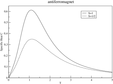
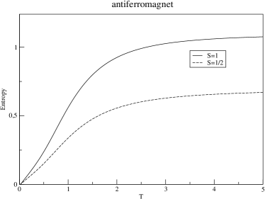
Figure 4: Depiction of the temperature dependence of a) specific heat $c(T)$, and b) entropy $S(T)$ for the spin-1 (solid lines) and the spin-$1/2$ (dashed lines) quantum chains with antiferromagnetic exchange.

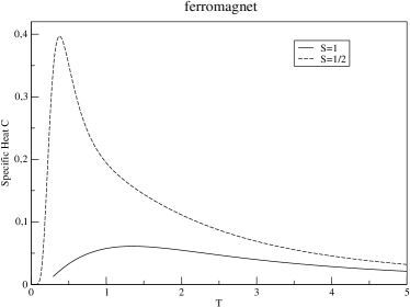
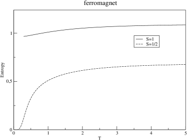
Figure 5: Depiction of the temperature dependence of a) specific heat $c(T)$, and b) entropy $S(T)$ for the spin-1 (solid lines) and the spin-$1/2$ (dashed lines) quantum chains with ferromagnetic exchange. Note that data for the spin-1 chain were not calculated to very low temperatures, see the main text for details.

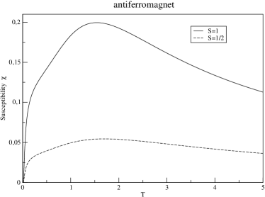
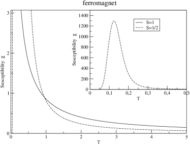
Figure 6: Depiction of the temperature dependence of the magnetic susceptibility $\chi(T)$ in case of a) antiferromagnetic exchange and b) ferromagnetic exchange for the spin-1 (solid lines) and the spin-$1/2$ (dashed lines) quantum chains. In the inset the full range of the susceptibility for the $XXZ$ chain is shown.

For the ferromagnetic case the numerical computations showed instabilities for the spin-1 chain. We attribute these instabilities to purely numerical causes and exclude physical reasons such as phase transitions. The data underlying the illustrations are those which were obtained within reasonable computation time. The specific heat in the ferromagnetic case looks similar to the antiferromagnetic case, however the order of the $S=1$ and the $S=1/2$ cases is inverted. This seems to contradict (129) and the high-temperature limits of the entropy $\log 3$ and $\log 2$. Note, however, that in the case of the spin-1 biquadratic model, one of the rare special cases with residual entropy is realized! Unlike the $S=1/2$ case and many other systems, for the ferromagnetic spin-1 biquadratic model and others of Sect. 2 the ground state is exponentially degenerate! The residual entropy is

$$S(T=0)=\log z=\log\left(\frac{d+\sqrt{d^{2}-4}}{2}\right),$$ (130)

which gives $S(T=0)=\log\left(3+\sqrt{5}\right)/2=0.9624...$ for dimension $d=3$ (and zero for $d=2$). This is also supported by the temperature dependence of the entropy as shown in figure 5b). The value of the residual entropy for $d=3$ was derived earlier [34]. Note that in the ferromagnetic ($S=1/2$) case, due to the larger excitation gap $\Delta E_{f}=2$, the thermodynamically activated behaviour at low temperatures is better visible than in the antiferromagnetic case.

In figure 6 the susceptibility $\chi(T)$ data are presented. For antiferromagnetic exchange coefficients, the $S=1$ and the $S=1/2$ cases look similar. The susceptibilities show a finite temperature maximum and approach zero for $T\to 0$ and $T\to\infty$. For the ferromagnetic case large values are obtained by $\chi(T)$ at low temperatures. For $T\to 0$ however, $\chi(T)$ drops to 0 again due to the finite excitation gap. This is observed for the $S=1/2$ chain. Unfortunately, for $S=1$ the true low-$T$ behaviour is not yet reached in the numerical treatment. On physical grounds, however, we expect a drop of $\chi(T)$ to 0 for low $T$.

6 Summary

We have shown how to construct the irreducible invariant subspaces (sectors) of Temperley-Lieb models in the case of open as well as periodic boundary conditions. A central step in the construction of the sectors was the identification of the one-dimensional representations of the (open as well as periodically closed) Temperley-Lieb algebra for arbitrary chain length.

The one-dimensional representations are also known as Bethe ansatz reference states. In the periodically closed case, the reference states had to be translationally invariant for being compatible with the boundary conditions. The questions about the eigenvalues and multiplicities (!) of the momentum operator in Hilbert spaces of tensor-product type and of reduced type led to an interesting analysis with compact answer that we did not find in the literature, but think should exist already.

The above findings lead to sobering insight with respect to alternative approaches like the coordinate and the algebraic Bethe ansatz. The fact, that most of the reference states of the Temperley-Lieb models with periodic boundary conditions have non-zero momentum eigenvalues leads to the equivalence with the $XXZ$ chain with twisted boundary conditions where the twist is given by the momentum value. (Note that in an extreme case, also an imaginary twist angle appears). Further, the higher spin-$S$ quantum chains have exponentially degenerate ground-states. This should explain the failure of attempts of direct Bethe ansatz calculations [20, 21] to construct all eigenstates from just one standard reference state.

There are two types of applications of our results. We like to point out, that the complete understanding of the spectrum of Temperley-Lieb systems with periodic boundary conditions allows for a study of the conformal dimensions. Here, we did not follow this line of thoughts and leave it for future work. Most interesting with respect to applications in the theory of the spin quantum Hall effect are vertex models with super-symmetry, like $sl(n+1,n)$ and local $2n+1$ dimensional space corresponding to $TL(\lambda=1)$.

As an application of the complete knowledge of multiplicities we computed the thermodynamical properties of the quantum spin chains without magnetic field by a direct mapping of the partition function to that of the $XXZ$ chain. Such a treatment would have been possible already on the basis of results by [10, 11]. Interestingly, our alternative indirect approach to thermodynamics by taking a detour via a classical two-dimensional model with twisted boundary conditions allowed for a more transparent and more general treatment allowing for arbitrary, non-vanishing (!) external fields. The result of these investigations is a ‘Temperley-Lieb equivalence at finite temperature and finite field’. The specific heat, entropy and susceptibility data of the biquadratic model were explicitly calculated for arbitrary temperature. Especially the low-temperature properties are very interesting. In the ferromagnetic case the susceptibility data show large values at low temperatures.

Our investigations are extensive, but not complete. We hope to report elsewhere on a complete study of the low-temperature asymptotics of the quantum spin chains and on the complete treatment of the non-semisimple cases including the super-symmetric chains. Also, we expect a generalization of some results to systems based on other algebras or formulated on lattices different from a simple chain. In case of the Hecke algebra, the equivalent reference models will be those solvable by nested Bethe ansatz.

Acknowledgment: B.A. acknowledges financial support by the DFG research training group 1052 and by VolksWagen-Stiftung. The authors are grateful to E. Müller-Hartmann, H.-A. Wischmann and C. Trippe for scientific discussions. The figures illustrating the thermodynamics of the quantum chains were produced from data calculated by C. Trippe.

References

• [1] Temperley, H.N.V., Lieb, E.: Proc. R. Soc. Lond. A322, 251 (1971)
• [2] Baxter R J 1982 Exactly Solved Models in Statistical Mechanics (London: Academic)
• [3] P. Martin: Potts Models and Related Problems in Statistical Mechanics, World Scientific, (1991)
• [4] Jones, V.R.F.: Invent. Math. 72, 1 (1983)
• [5] Andrews, G.E, Baxter, R.J., Forrester, P.J. : J. Stat. Phys. 35, 193 (1984)
• [6] A.L. Owczarek and R.J. Baxter: A class of interaction-round-a-face models and its equivalence with an ice-type model, J. Stat. Phys. 49, 1093 (1987)
• [7] V. Pasquier, Nucl. Phys. B285 [FS19], 162 (1987); J. Phys. A 20, L1229 (1987); 5707 (1987)
• [8] A. Klümper: New results for $q$-state vertex models and the pure biquadratic spin-1 Hamiltonian, Europhys. Lett. 9, 815-820 (1989)
• [9] P. P. Kulish and N. Reshetikhin: Quantum linear problem for the sine-Gordon equation and higher representations, Zap. Nauch. Semin. LOMI, 101, 101-110 (1981); Jour. Sov. Math. N4 (1983)
• [10] P. P. Kulish: On spin systems related to the Temperley-Lieb algebra, J. Phys. A: Math. Gen. 36 L489-L493 (2003)
• [11] P. P. Kulish, N. Manojlovic and Z. Nagy: Quantum symmetry algebras of spin systems related to Temperley-Lieb R-matrices, J. Math. Phys. 49 (2008)
• [12] Parkinson J B: J . Phys. C: Solid State Phys. 20 L1029 (1987); J . Phys. C: Solid State Phys. 21 3793 (1988); J . Physique C8 49, 1413 (1988)
• [13] Barber M and Batchelor M T: Phys. Rev. B 40, 4621 (1989)
• [14] Bazhanov, V. V. and Reshetikhin, N. Yu.: Critical RSOS models and conformal field theory, Int. J. Mod. Phys. A, 4 115-142 (1989)
• [15] P. Martin and H. Saleur: On An Algebraic Approach To Higher Dimensional Statistical Mechanics, Commun. Math. Phys. 158, 155–190, (1993)
• [16] P. Martin and H. Saleur: The blob algebra and the periodic Temperley-Lieb algebra, Letters in Mathematical Physics 30, 189-206 (1994)
• [17] A. Klümper: The spectra of $q$-state vertex models and related antiferromagnetic quantum spin chains. J. Phys. A 23, 809-823 (1990)
• [18] A. Klümper: Investigation of excitation spectra of exactly solvable models using inverson relations. Yang-Baxter Workshop/Conference, Canberra, Int. J. Mod. Phys. B 4, 871 (1990)
• [19] Alcaraz, F. C., Köberle, R. and Lima-Santos, A.: All Exactly Solvable U(1)-Invariant Quantum Spin 1 Chains from Hecke Algebra, Int. Journ. of Modern Physics A 7, 7615 (1992)
• [20] R. Köberle and A. Lima-Santos: Exact solutions for the deformed biquadratic spin-1 chain J.Phys. A27, 5409-5423 (1994)
• [21] R. Köberle and A. Lima-Santos: Exact solutions for A-D Temperley-Lieb models, J. Phys. A: Math. Gen. 29, 519–531 (1996)
• [22] D. Levy: Phys.Rev.Lett. 67, 1971 (1991)
• [23] V. Pasquier and H. Saleur: Common structures between finite systems and conformal field theories through Quantum Groups, Nucl. Phys. B330, 523-556 (1990)
• [24] F.M. Goodman, P. de la Harpe, and V.F.R. Jones: Coxeter Graphs and Towers of Algebras, Springer Verlag, (1989)
• [25] B. W. Westbury: The representation theory of the Temperley-Lieb algebras, Math. Z. 219, 539-565 (1995)
• [26] A. Nichols: The Temperley-Lieb algebra and its generalizations in the Potts and XXZ models, J. Stat. Mech. (2006)
• [27] F.C. Alcaraz, M.N. Barber, M.T. Batchelor, R.J. Baxter, and G.R.W. Quispel: Surface exponents of the quantum XXZ, Ashkin-Teller and Potts models, J. Phys. A: Math. Gen. 20, 6397–6409 (1987)
• [28] Sørensen, E. S.; Young, A. P.: Correlation length of the biquadratic spin-1 chain, Phys. Rev. B 42, 754-759 (1990)
• [29] C. D. Batista and A. A. Aligia: Exact Bond Ordered Ground State for the Transition between the Band and the Mott Insulator, Phys. Rev. Lett. 92, 246405 (2004)
• [30] Alcaraz, F. C. and Malvezzi, A. L. - On the Critical Behaviour of the Anisotropic Biquadratic Spin-1 Chain - J. Phys. A: Math. Gen. 25, 4535 (1992).
• [31] G. Albertini: Is the purely biquadratic spin 1 chain always massive? cond-mat/0012439 (December 2000)
• [32] A. Klümper: Thermodynamics of the anisotropic spin-1/2 Heisenberg chain and related quantum chains Z. Phys. B 91, 507-519 (1993)
• [33] A. Klümper: Free energy and correlation lengths of quantum chains related to restricted solid-on-solid lattice models Ann. Phys. 1, 540-553 (1992)
• [34] E. Müller-Hartmann: unpublished results (1989)