MISO Capacity with Per-Antenna Power Constraint

Abstract

We establish in closed-form the capacity and the optimal signaling scheme for a MISO channel with per-antenna power constraint. Two cases of channel state information are considered: constant channel known at both the transmitter and receiver, and Rayleigh fading channel known only at the receiver. For the first case, the optimal signaling scheme is beamforming with the phases of the beam weights matched to the phases of the channel coefficients, but the amplitudes independent of the channel coefficients and dependent only on the constrained powers. For the second case, the optimal scheme is to send independent signals from the antennas with the constrained powers. In both cases, the capacity with per-antenna power constraint is usually less than that with sum power constraint.

I Introduction

The capacity of a MIMO wireless channel depends on the constraints on the transmit power and on the availability of the channel state information at the transmitter and the receiver. With sum power constraint across all transmit antennas, the capacity and the optimal signaling are well established. For channels known at both the transmitter and the receiver, the capacity can be obtained by performing singular value decomposition of the channel and water-filling power allocation on the channel eigenvalues [1]. For Rayleigh fading channels with coefficients known only at the receiver, the ergodic capacity is obtained by sending independent signals with equal power from all transmit antennas [2].

Under the per-antenna power constraint, the MIMO capacity is less well understood. This per-antenna power constraint, however, is more realistic in practice than sum power because of the constraint on the individual RF chain connected to each antenna. Hence the transmitter may not be able to allocate power arbitrarily among the transmit antennas. Another appealing scenario for the per-antenna constraint is a distributed MIMO system, which has the transmitted antennas located at different physical nodes that cannot share power with each other. Thus understanding the capacity and the optimal signaling schemes under the per-antenna power constraint can be useful.

The per-antenna power constraint has been investigated in different problem setups. In [3], the problem of a multiuser downlink channel is considered with per-antenna power constraint. It was argued that linear processing at both the transmitter (by multi-mode beamforming) and the receiver (by MMSE receive beamforming with successive interference cancellation) can achieve the capacity region. Using uplink-downlink duality, the boundary points of the capacity region for the downlink channel with per-antenna constraint can be found by solving a dual uplink problem, which maximizes a weighted sum rate for the uplink channel with sum power constraint across the users and an uncertain noise. The dual uplink problem is convex which facilitates computation. In [4], an iterative algorithm based on geometric programming is proposed for maximizing the weighted sum rate of multiple users with per-antenna power constraint. In [5], another iterative method is proposed for solving the sum rate maximization problem under the more generalized power constraints on different groups of antennas. However, in all of these works, because of the complexity of the optimization problem, no closed-form analytical solutions of the optimal linear transmit processing scheme or the capacity were proposed. To the best of our knowledge, such closed-form solutions (for a MIMO channel with per-antenna power constraint) are not available even in the single-user case.

In this letter, we establish in closed-form the capacity and optimal signaling scheme for the single-user MISO channel with per-antenna power constraint. In this channel, the transmitter has multiple antennas and the receiver has a single antenna. Both cases of constant channel known to both the transmitter and receiver and of Rayleigh fading channel known only to the receiver are considered. When the channel is constant and known at both the transmitter and receiver, it turns out that the capacity optimal scheme is single-mode beamforming with the beam weights matched to the channel phases but not the channel amplitudes. Our result covers the special case of 2 transmit antennas considered in [6] as part of a Gaussian multiple access channel channels with common data, in which it was established that beamforming of the common data only maximizes the sum rate, which is equivalent to beamforming in a MISO channel. When the channel is Rayleigh fading and is known only to the receiver, the optimal scheme is sending independent signals from the transmit antennas with the constrained powers. In both cases, the capacity with per-antenna power constraint is usually less than that with sum power constraint.

In establishing these results, we need to solve the corresponding capacity optimization problems. In the constant channel case, our proof method is to solve a relaxed problem and then show that the solution of the relaxed problem satisfies the original constraints and hence is optimal. In the fading channel case, our proof is based on the symmetry of the Raleigh fading distribution. This latter technique can be generalized directly to the MIMO fading channel with per-antenna power constraint.

The rest of this letter is organized as follows. In Section II, we discuss the MISO channel model, the capacity optimization problem and the different power constraints. Then the results for constant channels known at both the transmitter and receiver are established in Section III, and for Rayleigh fading channels known only at the receiver in Section IV. In Section V, we provide some concluding remarks. For notation, we use bold face lower-case letters for vectors, capital letters for matrices, $(.)^{T}$ for transpose, $(.)^{\ast}$ for conjugate, $(.)^{\dagger}$ for conjugate transpose, $\succcurlyeq$ for matrix inequality (positive semi-definite relation), $\text{tr}(.)$ for trace, and ${\text{diag}}\{.\}$ for forming a diagonal matrix with the specified elements.

II Channel Model and Power Constraints

II-A Channel model

Consider a multiple-input single-output (MISO) channel with $n$ transmit antennas. Assuming flat-fading, the channel from each antenna is a complex, multiplicative factor $h_{i}$. Denote the channel coefficient vector as ${\mathbf{h}}=[h_{1}\ldots h_{n}]^{T}$, and the transmit signal vector as ${\bf x}=[x_{1}\ldots x_{n}]^{T}$. Then the received signal can be written as

$$y={\bf h}^{T}{\bf x}+z$$ (1)

where $z$ is a scalar additive white complex Gaussian noise with power $\sigma^{2}$.

We assume that the channel coefficient vector ${\bf h}$ is known at the receiver, which is commonly the case in practice with sufficient receiver channel estimation. We consider 2 cases of channel information at the transmitter: constant channel coefficients also known to the transmitter, and fading channel coefficients which are circularly complex Gaussian and are not known to the transmitter. The former can correspond to a slow fading environment, whereas the latter applies to fast fading.

The capacity of this channel depends on the power constraint on the input signal vector ${\bf x}$. In all cases, however, because of the Gaussian noise and known channel at the receiver, the optimal input signal is Gaussian with zero mean [2]. Let ${\bf Q}=E[{\bf xx}^{\dagger}]$ be the covariance of the Gaussian input, then the achievable transmission rate is

$$R=\log\left(1+\frac{1}{\sigma^{2}}{\bf h}^{T}{\bf Q}{\bf h}^{\ast}\right).$$ (2)

The remaining question is to establish the optimal ${\bf Q}$ that maximizes this rate according to a given power constraint.

II-B Power constraints

Often the MISO channel is studied with sum power constraint across all antennas. In this letter, we study a more realistic per-antenna power constraint. For comparison, we also include the case of independent multiple-access power constraint. We elaborate on each power constraint below.

II-B1 Sum power constraint

With sum power constraint, the total transmit power from all $n$ antennas is $P$, but this power can be shared or allocated arbitrarily among the transmit antennas. This constraint translates to the condition on the input covariance as $\text{tr}({\bf Q})\leq P$.

II-B2 Independent multiple-access power constraint

In this case, each transmit antenna has its own power budget and acts independently. This constraint can model the case of distributed transmit antennas, such as on different sensing nodes scattered in a field, without explicit cooperation (in terms of coding and signal design) among them. Let $P_{i}$ be the power constraint on antenna $i$, then this constraint is equivalent to having a diagonal input covariance ${\bf Q}={\text{diag}}\{P_{1},\ldots,P_{n}\}$.

II-B3 Per-antenna power constraint

Here each antenna has a separate transmit power budget of $P_{i}$ ($i=1,\ldots,n$) and can fully cooperate with each other. Such a channel can model a physically centralized MISO system, for example, the downlink of a system with multiple antennas at the basestation and single antenna at each user. In such a centralized system, the per-antenna power constraint comes from the realistic individual constraint of each transmit RF chain. The channel can also model a distributed (but cooperative) MISO system, in which each transmit antenna belongs to a sensor or ad hoc node distributed in a network. In such a distributed scenario, the nodes have no ability to share or allocate power among themselves and hence the per-antenna power constraint holds (but they may wish to cooperate to design codes and transmit signals). The per-antenna constraint is equivalent to having the input covariance matrix ${\bf Q}$ with fixed diagonal values $q_{ii}=P_{i}$. Note that this constraint is on the diagonal values of ${\bf Q}$ and is not the same as having the eigenvalues of ${\bf Q}$ equal to $P_{i}$.

III MISO capacities with constant channels

In this section, we investigate the case that the channel is constant and known at both the transmitter and the receiver. First, we briefly review known results on the capacity of the channel in (1) under sum power constraint and independent multiple access constraint. Then we develop the new result on MISO capacity with per-antenna power constraint.

III-A Review of known capacity results

III-A1 MISO capacity under sum power constraint

With sum power constraint, the capacity optimization problem can be posed as

$$\max \log\left(1+\frac{1}{\sigma^{2}}{\bf h}^{T}{\bf Q}{\bf h}^{\ast}\right)$$ (3)

s.t. $$\text{tr}({\bf Q})\leq P\;,\quad{\bf Q}\succcurlyeq 0$$

where ${\bf Q}$ is Hermitian. This problem is convex in ${\bf Q}$. Let ${\bf Q}={\bf U\Lambda U}^{\dagger}$ be the eigenvalue decomposition, then the optimal solution is to pick an eigenvector ${\bf u}_{1}={\bf h}^{\ast}/\|{\bf h}\|$ and allocate all transmit power in this direction, that is, the first eigenvalue $\lambda_{1}=P$.

Thus the transmitter performs single-mode beamforming with the optimal beam weights as ${\bf h}^{\ast}/\|{\bf h}\|$. At each time, all transmit antennas send the same symbol weighted by a specific complex weight at each antenna. In this optimal beamforming, the beam weight on an antenna not only has the phase matched to (being the negative of) the phase of the channel coefficient from that antenna, but also the amplitude proportional to the amplitude of that channel coefficient. In other words, power is allocated among the antennas proportionally to the channel gains from these antennas.

The MISO capacity with sum power constraint is

$$C_{s}=\log\left(1+\frac{P}{\sigma^{2}}\sum_{i=1}^{n}|h_{i}|^{2}\right)=\log\left(1+\frac{P}{\sigma^{2}}\|{\bf h}\|^{2}\right).$$ (4)

III-A2 Independent multiple-access capacity

Under the independent multiple-access constraint, the capacity is equivalent to the sum capacity a multiple access channel, without explicit cooperation among the transmitters, as [1]

$$C_{ma}=\log\left(1+\frac{1}{\sigma^{2}}\sum_{i}P_{i}|h_{i}|^{2}\right).$$ (5)

In this case, there is no optimization since ${\bf Q}=\text{diag}\{P_{1},\ldots,P_{n}\}$. The transmit antennas send different and independent symbols at each time.

III-B MISO capacity with per-antenna power constraint

The capacity with per-antenna power constraint can be found by solving the following optimization problem:

$$\max \log\left(1+\frac{1}{\sigma^{2}}{\bf h}^{T}{\bf Q}{\bf h}^{\ast}\right)$$ (6)

s.t. $$q_{ii}\leq P_{i}\quad i=1,2,\ldots,n$$

$${\bf Q}\succcurlyeq 0.$$

Noting that the per-antenna power constraint $q_{ii}\leq P_{i}$ can be written as ${\bf e}_{i}^{T}{\bf Q}{\bf e}_{i}\leq P_{i}$ where ${\bf e}_{i}=[0\ldots 1\ldots 0]^{T}$ is a vector with the $i^{\text{th}}$ element equal to $1$ and the rest is $0$, thus this constraint is linear in ${\bf Q}$. Thus the above problem is also convex. So far, however, there is no closed-form solution available.

We are able to solve the above problem (6) analytically with closed-form solution by first applying a matrix minor condition to relax the positive semi-definite constraint ${\bf Q}\succcurlyeq 0$, reducing the problem to a form solvable in closed-form, and then showing that the optimal solution to the relaxed problem is also the optimal solution to the original problem. The details are given in Appendix -A.

It is also possible to show that the optimal covariance of (6) has the rank satisfying $\text{rank}({\bf Q}^{\star})\leq\text{rank}({\bf h})$. Hence for the MISO channel considered here, $\text{rank}({\bf Q}^{\star})=1$ and the optimal signaling is beamforming. This proof is provided in Appendix -B.

Here we describe the optimal covariance ${\bf Q}^{\star}$ and discuss the meaning of the solution. The optimal ${\bf Q}^{\star}$ has the elements given as

$$q_{ij}=\frac{h_{i}^{\ast}h_{j}}{|h_{i}h_{j}|}{\sqrt{P_{i}P_{j}}}\;,\quad i,j=1,\ldots,n.$$ (7)

Let ${\bf Q}^{\star}={\bf V\Lambda V}^{\dagger}$ be its eigenvalue decomposition. ${\bf Q}^{\star}$ can be shown to have rank-one with the single non-zero eigenvalue as $\lambda_{1}=\sum P_{i}$ and the corresponding eigenvector ${\bf v}_{1}$ with elements given as

$$v_{k1}=\frac{h_{k}^{\ast}}{|h_{k}|}\frac{\sqrt{P_{k}}}{\sqrt{P}}=\eta_{k}\frac{\sqrt{P_{k}}}{\sqrt{P}}$$ (8)

where $P=\sum P_{i}$ and $\eta_{k}=h_{k}^{\ast}/|h_{k}|$ is a point on the complex unit circle with phase as the negative of the phase of $h_{k}$.

The optimal signaling solution with per-antenna power constraint is beamforming with the beam weight vector as ${\bf v}_{1}^{\ast}$. Different from the sum power constraint case, here, the beam weight only has the phase matched to the phase of the channel coefficient, but the amplitude independent of the channel and fixed according to the power constraint. Thus there is no power allocation among the transmit antennas: the transmit power from the $i^{th}$ antenna is fixed as $P_{i}$.

For beamforming, it is useful to examine the angle $\theta$ ($0\leq\theta\leq\pi/2$) between a beam weight vector ${\bf w}$ and the channel vector ${\mathbf{h}}$, defined as $\cos\theta={\bf h}^{\dagger}{\bf w}/(\|{\bf h}\|\cdot\|{\bf w}\|)$. This angle $\theta$ affects the capacity as follows:

$$C_{p} =\log\left(1+\frac{1}{\sigma^{2}}P\|{\bf h}\|^{2}\cos\theta\right).$$ (9)

Hence the smaller the angle, the larger the capacity. As in the case with sum-power constraint, the beam weight ${\bf w}={\bf h}^{\ast}/\|{\bf h}\|$ completely matches the channel (both the phase and amplitude) and the capacity as obtained in (4) is the maximum.

With per-antenna power constraint, the beam-weight vector is ${\bf w}={\bf v}_{1}$ and the angle $\theta$ satisfies

$$\cos\theta=\sum_{k}\frac{h_{k}}{|h_{k}|}\frac{\sqrt{P_{k}}}{\sqrt{P}}\frac{h_{k}^{\ast}}{|h|}=\frac{1}{|h|\sqrt{P}}\sum_{k}|h_{k}|\sqrt{P_{k}}.$$ (10)

Applying the Cauchy-Schwartz’s inequality on (10), the maximum $\cos\theta=1$ occurs if and only if $\sqrt{P_{k}}=c|h_{k}|$ for some constant $c$ and for all $k=1,\ldots,n$. In all other cases, $\cos\theta<1$ and hence $\theta>0$. Thus with the per-antenna power constraint, except for the special case in which the power constraints $P_{i}$ happens to be proportional to the channel coefficient amplitude $|h_{i}|$, the beamforming vector ${\bf v}_{1}^{\ast}$ does not completely align with the channel vector ${\bf h}$. Nevertheless, it provides the largest transmission rate without power allocation.

Our result also covers the case of 2 user multiple access channel with common data considered in [6], which states that the sum rate is maximized by just sending the common data and performing beamforming.

The MISO capacity with per-antenna power constraint is

$$C_{p}=\log\left[1+\frac{1}{\sigma^{2}}\left(\sum_{i=1}^{n}|h_{i}|\sqrt{P_{i}}\right)^{2}\right].$$ (11)

Compared to (4) and (5), we see that $C_{ma}\leq C_{p}\leq C_{s}$.

III-C Numerical examples

III-C1 With 2 transmit antennas

We provide numerical examples of the capacities for a MISO channel with 2 transmit antennas. Assume a complex test channel ${\bf h}=[0.3+0.2i\;\;0.4-0.7i]^{T}$. For fair comparison, the total transmit power in the sum power constraint must equal the sum of the individual powers in the per-antenna power constraint. Thus we choose the transmit powers such that $P_{1}+P_{2}=P=10$.

Figure 1 shows the MISO capacity versus $P_{1}$ under the three different power constraints: sum power constraint (4), independent multiple-access power constraint (5), and per-antenna power constraint (11). Compared to the multiple access capacity which is obtained with independent signals from the different transmit antennas, we see that introducing correlation among the transmit signals by beamforming increases the capacity. (Single-mode beamforming introduces complete correlation among the signals from different antennas since all antennas send the same symbol, just with different weights.) Under the sum power constraint, power allocation can further increase the capacity.

The two MISO capacities with sum power constraint and per-antenna power constraint are equal at a single point when the value of $P_{1}$ is such that $P_{1}/P_{2}=|h_{1}|^{2}/|h_{2}|^{2}$, which is $P_{1}^{\star}=1.72$ in this example. On the other hand, at the equal power point $P_{1}=P_{2}=5$, the capacity with per-antenna power constraint is about 93% of that with sum power constraint, and is almost 30% higher than the multiple access capacity.

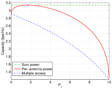
Figure 1: Capacities for a $2\times 1$ constant channel under different power constraints.

III-C2 With $n$ transmit antennas

With $n$ transmit antennas ($n>2$), it is more informative to study the capacity as a function of $n$. To make some insightful comparisons, we consider the case in which all users have the same transmit power budget $P_{i}=P_{0}=1$ and $\sigma^{2}=1$. We can see that if the channel is also symmetric ($h_{i}=h_{j}$ for all $i,j$) then the capacity with per-antenna power constraint is the same as that with sum power constraint. Now suppose that the channel is non-symmetric as $h_{k}=k$. Then the 3 capacities become

$${\cal C}_{ma} =\log\left(1+\frac{P_{0}}{\sigma^{2}}\left(\frac{n^{3}}{3}+\frac{n^{2}}{2}+\frac{n}{6}\right)\right)$$

$${\cal C}_{p} =\log\left(1+\frac{P_{0}}{\sigma^{2}}\frac{(n^{2}+n)^{2}}{4}\right)$$

$${\cal C}_{s} =\log\left(1+\frac{nP_{0}}{\sigma^{2}}\left(\frac{n^{3}}{3}+\frac{n^{2}}{2}+\frac{n}{6}\right)\right).$$

Figure 2 shows these capacities versus the number of users $n$. In this case, the capacity with per-antenna power constraint is almost as high as the capacity with sum power constraint, and both are significantly better than the multiple access capacity.

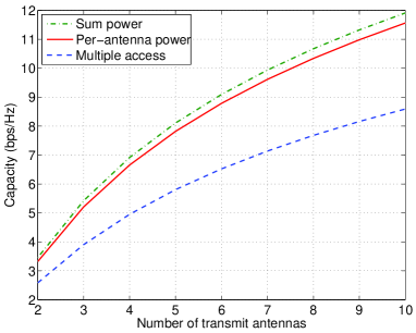
Figure 2: Sum capacity for the power symmetric case with $h_{k}=k$.

IV MISO capacities with fading channels

In this section, we study Rayleigh fading channels, in which the channel coefficients $h_{i}$ are now independent, zero-mean complex circularly Gaussian random variables with unit variance. We assume that the channel vector ${\bf h}$ is known perfectly to the receiver but is unknown to the transmitter.

Again we first review the known capacity results with sum power constraint and independent multiple access power constraint, then establish the new result with per-antenna power constraint.

IV-A Review of known capacity results

IV-A1 MISO capacity with sum power constraint

For a MISO fading channel with sum power constraint, the capacity is a special case of [2]. The optimal covariance of the Gaussian transmit signal is ${\bf Q}=\frac{P}{n}{\bf I}$, implying that each antenna sends independent signal with equal power. The ergodic MISO capacity is

$${\cal C}_{s}=E_{{\bf h}}\left[\log\left(1+\frac{P}{n\sigma^{2}}\|{\bf h}\|^{2}\right)\right].$$ (12)

Compared to (4), there is a dividing factor of $n$ in the power in the instantaneous capacity equation. This power loss factor is due to the lack of channel information at the transmitter.

IV-A2 Independent multiple-access capacity

In this case, the transmit covariance is ${\bf Q}=\text{diag}\{P_{1},\ldots,P_{n}\}$. The capacity is obtained by averaging the instantaneous capacity in (5) over fading [7]. Specifically, the ergodic capacity is

$${\cal C}_{ma}=E_{{\bf h}}\left[\log\left(1+\frac{1}{\sigma^{2}}\sum_{i=1}^{n}P_{i}|h_{i}|^{2}\right)\right].$$ (13)

IV-B MISO capacity with per-antenna power constraint

To establish the ergodic MISO capacity with per-antenna power constraints, we need to solve the following stochastic version of problem (6):

$$\max E_{{\bf h}}\left[\log\left(1+\frac{1}{\sigma^{2}}{\bf h}^{T}{\bf Q}{\bf h}^{\ast}\right)\right]$$ (14)

s.t. $${\bf Q}\succcurlyeq 0\;,\quad q_{ii}\leq P_{i}\;,\quad i=1,\ldots,n,$$

where ${\bf Q}$ is Hermitian.

Since the per-antenna constraint $q_{ii}\leq P_{i}$ is not the same as a constraint on the eigenvalues of ${\bf Q}$, the analysis for fading channels as in [2] cannot be applied here. That is, if we perform the eigenvalue decomposition ${\bf Q}={\bf U}_{Q}{\bf\Lambda}_{Q}{\bf U}_{Q}^{\dagger}$, then although ${\bf h}^{T}{\bf U}_{Q}$ has the same distribution as ${\bf h}^{T}$, the diagonal values of ${\bf\Lambda}_{Q}$ do not have the same constraints as the diagonal values of ${\bf Q}$. Hence the problem is no longer equivalent through eigen-decomposition.

However, by also relying on the centrality and symmetry of the Rayleigh fading distribution in a slightly different way, we show that the optimal solution of (14) is ${\bf Q}=\text{diag}\{P_{1},\ldots,P_{n}\}$. The details are given in Appendix -C.

The optimal solution means that each transmit antenna sends independent signal at its full power. Somewhat surprisingly, this is the same transmit strategy under the independent multiple access constraint. Hence the ergodic capacity with per-antenna power constraint is

$${\cal C}_{p}={\cal C}_{ma}.$$ (15)

Thus, for a Rayleigh fading without channel information at the transmitter, having the possibility for cooperation among the transmit antennas under the per-antenna power constraint does not increase the average capacity. (It should be noted, however, that cooperation without transmit channel state information can still increase reliability significantly [8].)

From (12), (13) and (15), we can show that

$${\cal C}_{p}\leq{\cal C}_{s}$$ (16)

always holds. This is proven by noticing that the channel coefficients $h_{i}$ are i.i.d. Thus for any permutation $\pi=\text{perm}(1,\ldots,n)$, we can express ${\cal C}_{p}$ as

$${\cal C}_{p}=E_{{\bf h}}\left[\log\left(1+\frac{1}{\sigma^{2}}\sum_{i=1}^{n}P_{i}|h_{\pi_{i}}|^{2}\right)\right].$$

Let $\pi^{(k)}=(k,\ldots,n,1,\ldots,k-1)$ which is a rotation of the order. Then based on the concavity of the $\log$ function, the following expressions holds:

$${\cal C}_{p} =\frac{1}{n}\sum_{k=1}^{n}E_{{\bf h}}\left[\log\left(1+\frac{1}{\sigma^{2}}\sum_{i=1}^{n}P_{i}|h_{\pi^{(k)}_{i}}|^{2}\right)\right]$$

$$\leq E_{{\bf h}}\left[\log\left(1+\frac{1}{n}\sum_{k=1}^{n}\frac{1}{\sigma^{2}}\sum_{i=1}^{n}P_{i}|h_{\pi^{(k)}_{i}}|^{2}\right)\right]={\cal C}_{s}.$$

Equality holds if and only if $P_{i}=P/n$ for all $i$.

We see that similar to the case of sum power constraint, under the per-antenna power constraint, the presence or lack of channel information at the transmitter has a significant impact on the optimal transmit strategy and the channel capacity. With full channel state information, the optimal strategy under either power constraint is beamforming (sending completely correlated signals), while without channel state information at the transmitter, the optimal strategy is to send independent signals from the different antennas.

IV-C Numerical examples

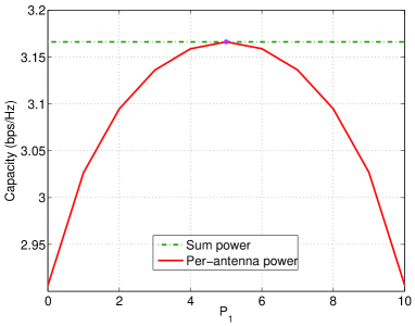
Figure 3: Ergodic capacities for a $2\times 1$ Rayleigh fading channel under different power constraints.

For numerical example, we examine a MISO fading channel with 2 transmit antennas. Figure 3 shows the plots of the ergodic capacities in (12), (13) and (15) versus the transmit power constraint on the first antenna. The symmetry observed in these plots is a result of the average over fading. The difference in the ergodic capacities with sum power constraint and with per-antenna power constraint are smaller in fading channels than in constant channels. The two capacities are equal at the point $P_{1}=P/2=5$.

V Conclusion

We have established the MISO capacity with per-antenna power constraint for 2 cases of channel state information. In the case of constant channel known to both the transmitter and the receiver, the capacity is obtained by beamforming. The optimal beam weights, however, are different from those under the sum power constraint. Specifically, only the phases of the beam weights are matched to the phases of the channel coefficients, but the amplitudes are independent of the channel and depend only on the constrained powers. In the case of Rayleigh fading channel known to the receiver only, the capacity is obtained by sending independent signals from the transmit antennas with the constrained powers. In both cases, the capacity with per-antenna power constraint is usually less than that with sum power constraint.

Our proof technique for the case of Rayleigh fading channel can be applied directly to the more general MIMO fading channel with per-antenna power constraint. For the case of constant channel known at both the transmitter and receiver, however, the proof technique here may not be generalized directly to the MIMO channel, except that of the rank. The capacity of a constant MIMO channel with per-antenna constraint is still an open problem.

References

- [1] T. Cover and J. Thomas, Elements of Information Theory, 2nd ed. John Wiley & Sons, Inc., 2006.
- [2] I. Telatar, “Capacity of multi-antenna Gaussian channels,” European Transactions on Telecommunications, vol. 10, no. 6, pp. 585–595, Nov 1999.
- [3] W. Yu and T. Lan, “Transmitter optimization for the multi-antenna downlink with per-antenna power constraints,” IEEE Transactions on Signal Processing, vol. 55, no. 6, pp. 2646–2660, Jun 2007.
- [4] S. Shi, M. Schubert, and H. Boche, “Per-antenna power constrained rate optimization for multiuser MIMO systems,” in International ITG Workshop on Smart Antennas (WSA), 2008, pp. 270–277.
- [5] M. Codreanu, A. Tolli, M. Juntti, and M. Latva-aho, “MIMO downlink weighted sum rate maximization with power constraints per antenna groups,” in IEEE VTC Spring, 2007, pp. 2048–2052.
- [6] N. Liu and S. Ulukus, “Capacity region and optimum power control strategies for fading Gaussian multiple access channels with common data,” IEEE Transactions on Communications, vol. 54, no. 10, pp. 1815–1826, Oct 2006.
- [7] S. Shamai and A. Wyner, “Information-theoretic considerations for symmetric, cellular, multiple-access fading channels. II,” IEEE Transactions on Information Theory, vol. 43, no. 6, pp. 1895–1911, Nov 1997.
- [8] J. Laneman and G. Wornell, “Distributed space-time coded protocols for exploiting cooperative diversity in wireless networks,” IEEE Transactions on Info. Theory, vol. 49, no. 10, pp. 2415–2425, Oct 2003.
- [9] J. Prussing, “The principal minor test for semidefinite matrices,” Journal of Guidance, Control and Dynamics, vol. 9, no. 1, pp. 121–122, Jan-Feb 1986.
- [10] R. F. H. Fischer, Precoding and Signal Shaping for Digital Transmission. Wiley-IEEE Press, 2002.
- [11] H. Van Trees, Optimum Array Processing (Detection, Estimation, and Modulation Theory, Part IV). New York: Wiley, 2002.