Naked Singularity Formation In Brans-Dicke Theory

Abstract

Gravitational collapse of the Brans-Dicke scalar field with non-zero potential in the presence of matter fluid obeying the barotropic equation of state, $p=w\rho$ is studied. Utilizing the concept of expansion parameter, it is seen that the cosmic censorship conjecture may be violated for $w=-\frac{1}{3}$ and $w=-\frac{2}{3}$ which correspond to cosmic string and domain wall, respectively. We show that physically, it is the rate of collapse and the presence of Brans-Dicke scalar field that govern the formation of a black hole or a naked singularity as the final fate of dynamical evolution and only for these two cases the singularity can be naked as the collapse end state. Also the weak energy condition is satisfied by the collapsing configuration.

I Introduction

The process of gravitational collapse has been studied since about 60 years ago as a solution of Einstein field equations. When a sufficiently massive star many times the size of the Sun exhausts its nuclear fuel without reaching an equilibrium state such as a neutron star or white dwarf, it collapses under its own pull of gravity at the end of its life cycle. Therefore, gravity overtakes and dominates the other three forces of nature, in particular, the weak and strong nuclear forces, which generically provide the outward pressure in a star to balance it against the inward pull of gravity. In such ultra-strong gravity regions the densities and spacetime curvature diverge and a spacetime singularity will be born, either hidden within an event horizon (a black hole) or visible to the external universe (a naked singularity), as predicted by the singulary theorems in general relativity. The visibility or otherwise of the singularity to outside observers is determined by the causal structure of the dynamically developing collapsing cloud as governed by the Einstein’s field equations. When the internal dynamics of the collapse delays the formation of the horizon, the singularity becomes visible, and may communicate physical effects to the external universe 01 .

Up until now a great deal of effort has gone into the study of the nature of singularities and large classes of the solutions of Einstein’s field equations treating singularities have been represented. The general and exact class of solutions of Einstein’s field equations describing spherically symmetric pressureless matter (dust) for motion with no particle layers intersecting, independent of the homogeneity assumption, was originally introduced by Lema$\hat{i}$tre 02 ; 03 in an attempt to describe cosmology, which was further developed and studied by Tolman 04 ; 05 and Bondi 04 ; 06 . This class could be used to model the gravitational collapse of matter from general inhomogeneous initial conditions and the end state of gravitational collapse of a massive star can be studied within this framework 04 . Contrary to the collapsing Friedmann case, in which the physical singularity occurs at a constant epoch of time, namely at $t=0$, the singular epoch (the time $t=t_{0}(r)$ at which the area radius of the collapsing shell of matter at a constant value of the co-moving coordinate r vanishes) in LTB model is a function of r as a result of inhomogeneity in the matter distribution. This model can exhibit two kinds of naked singularity: a shell-crossing 07 ; 08 and a shell-focussing singularity 07 ; 09 ; 10 . These kinds of naked singularity are generic for spherical dust collapse and with proper choice of initial data they are globally naked. The main reason which causes this model to be deficient is that it neglects the pressure, which is likely to diverge at these singularities (where the density diverges) 07 . A special case of these classes of solutions which has served as the basic paradigm in black hole physics is the Oppenheimer-Synder study of a completely homogeneous, pressure-free and spherically symmetric dust cloud collapse, where a dust cloud undergoes a continued collapse which commences from regular initial data (i.e., there is no trapped surfaces forming at the initial spacelike surface from which the collapse begins and the light rays can escape from the surface of the star to faraway observers) to form a black hole 04 ; 11 ; 12 . Most of our knowledge about the gravitational collapse is still based on that model. Also it describes well the formation of the horizon and evolution of the central, space-like singularity. Oppenheimer and Snyder analyzed the causal structure of the solution by considering in particular an observer on the surface of the dust cloud sending signals to a faraway stationary observer at regularly spaced intervals as measured by his own clock. They discovered that as the radius of the dust cloud approaches $2M$, the spacing between the arrival times of these signals to the faraway observer becomes progressively longer, tending to infinity. This effect has since been called the infinite redshift effect. The observer on the surface of the dust cloud may keep sending signals after its radius has become less than $2M$, but these signals can not escape from this region since the speed of light is the limiting propagation velocity for physical signals. within a finite affine parameter interval, these signals reach a true singularity at $r=0$ 13 . This singularity is formed inside a black hole, as a final state of the collapse process and also accords to the concept of the cosmic censorship. The cosmic censorship conjecture which is initially represented by Penrose 14 , explain the properties of the final singularity of a gravitational collapse. The main result of this conjecture is that, all spacetime singularities arising from regular initial data that appear in a gravitational collapse (in an asymptotically flat universe) are always surrounded by an event horizon and hence invisible to outside observers (no naked singularities). Moreover in the strong version of this conjecture, such singularities are not even locally naked, i.e. there is not any timelike or null geodesics which can emerge from these singularities and go to future infinity 07 . This hypothesis plays a fundamental role in both the theory and applications of black hole physics and has been recognized as one of the most important open problems in classical general theory of relativity. Up to now many exact solutions of Einstein’s field equations with several kinds of field-sources which admit naked singularities depending upon the nature of the initial data and the kinematical properties near the singularity have been considered. The models studied so far include the collapse of scalar fields 15 ; 16 as well as other matter sources including dust 17 ; 18 ; 09 , radiation 17 ; 19 ; 10 , perfect fluid 17 ; 20 ; 07 , imperfect fluids 17 ; 21 , and null strange quark fluids 15 ; 22 .

One would like to inquire about what are the possible physical factors operating during the process of a continual collapse of a massive matter cloud which results in the formation of a naked singularity or a black hole as the collapse end state. Such an investigation should help us understand much better the physics of black holes and naked singularity formation in gravitational collapse. It was recently shown 23 ; 24 that for the spherical dust collapse the shearing effects and inhomogeneity present within the collapsing cloud do play a crucial role in delaying the formation of the trapped surfaces and the apparent horizon. These effects could in fact make the geometry of apparent and event horizons distorted sufficiently, which exposes the singularity to the external observers 23 .

General relativity is not the only gravitational theory which explain the gravitational phenomena. There are alternative theories of gravity that can explain the gravitational phenomena and lead to many interesting results and physical interpretations. One of those, is the scalar-tensor theory of gravity, which has been actively studied as an alternative and successful theory of gravity. Recently, they have attracted much attention, in part because they emerge naturally as the low-energy limit of many theories of quantum gravity, such as Kaluza-Klein theories25 ; 26 and supersymmetric string theories25 ; 27 . These theories are also important for ”extended” cosmological inflation models25 ; 28 , in which the scalar field allows the inflationary epoch to end via bubble nucleation without the need for fine-tuning cosmological parameters(the ”graceful exit” problem)29 . In Brans-Dicke theory, the simplest of scalar-tensor theories, gravitation is described by a metric $g_{\mu\nu}$ and a scalar field $\phi$ coupled to both matter and space time geometry which obeys a wave equation with a source term determined by the matter distribution. Gravitational collapse in this theory has been studied in some of the recent literature. In this paper we study the formation of naked singularity as the end state of gravitational collapse of a matter fluid obeying the barotropic equation of state, $p=w\rho$ in the context of Brans-Dicke (BD) theory. Being motivated by this concept, we investigate the violation of cosmic censorship conjecture in the collapse procedure of such a matter fluid.

II Basic equations

In the context of Brans-Dicke theory with a self interacting potential and a matter field, the action is given by

$${\mathcal{S}}=\frac{1}{2\kappa}\int d^{4}x\sqrt{-g}\left(\Phi R-\frac{\omega}{\Phi}\nabla^{\alpha}\Phi\nabla_{\alpha}\Phi-V(\Phi)\right)+{\mathcal{S}}_{m},$$ (1)

where the constant $\omega$ is the Brans-Dicke parameter and $\Phi$ is the Brans-Dicke scalar field, which is related to the gravitational ”constant” by $G=\frac{1}{\Phi}$. Extremizing the action yields the field equations(we set $\kappa=8\pi G=c=1$ in the rest of this paper)

$$G_{\mu\nu}=T^{({\rm eff})}_{\mu\nu},$$ (2)

where the effective stress-energy tensor is

$$T^{({\rm eff})}_{\mu\nu}=\frac{1}{\Phi}\left(T^{\rm m}_{\mu\nu}+T^{\Phi}_{\mu\nu}\right),$$ (3)

with

$$T^{\Phi}_{\mu\nu}=\frac{\omega}{\Phi}(\nabla_{\mu}\Phi\nabla_{\nu}\Phi-\frac{1}{2}g_{\mu\nu}\nabla^{\alpha}\Phi\nabla_{\alpha}\Phi)+(\nabla_{\mu}\nabla_{\nu}\Phi-g_{\mu\nu}\Box\Phi)-\frac{1}{2}g_{\mu\nu}V(\Phi),$$ (4)

and

$$T^{m}_{\mu\nu}={\rm diag}\left(\rho_{m},p_{m},p_{m},p_{m}\right),$$ (5)

being the stress-energy tensors of scalar field and matter fluid, respectively. Here we look at the BD scalar field as matter fields originating from geometry. Variation of the action with respect to $\Phi$ gives

$$\Box\Phi=\frac{T^{\rm m}}{2\omega+3}+\frac{1}{2\omega+3}\left(\Phi\frac{dV(\Phi)}{d\Phi}-2V(\Phi)\right).$$ (6)

where $T^{m}$ stands for the trace of $T^{m}_{\mu\nu}$ and the subscript ”$m$” refers to the matter fields (fields other that $\Phi$). In general relativity the interior solution of a collapsing star is given by the Tolman-Bondi solution. Here we present a transparent consideration of a homogenous collapsing star with BD scalar field $\Phi=\Phi(\tau)$ and effective potential $V=V(\Phi)$. With this consideration, the Tolman-Bondi solution converts to a Friedmann-Robertson-Walker(FRW) metric. The interior metric for marginally bound $(k=0)$ case is given by

$$ds^{2}=-d\tau^{2}+a^{2}(\tau)(dr^{2}+r^{2}d\Omega^{2}),$$ (7)

where $\tau$ is the proper time of free falling observer whose geodesic trajectories are distinguished by the comoving radial coordinate $r$ and $d\Omega^{2}$ being the standard line element on the unit two sphere. Since the presence of matter acting as a ”seed” field and origin of spherical symmetry, prompts the collapse of BD scalar field, we have considered perfect fluid models with barotropic equation of state being given by

$$p_{m}=w\rho_{m}.$$ (8)

Using the continuity equation for the matter and Eq. (8) one gets the following relations between $\rho_{m},~{}p_{m}$ and the scale factor as follows

$$\rho_{m}=\rho_{{}_{{}_{0}}m}a^{-3(1+w)};~{}~{}p_{m}=w\rho_{{}_{{}_{0}}m}a^{-3(1+w)},$$ (9)

where $\rho_{{}_{{}_{0}}m}=\rho_{m}(a=1)$, is the initial value of the energy density of matter on the collapsing shell. One then has the following equations for the effective stress-energy tensor

$$\rho_{{}_{({\rm eff})}}=T^{\tau}\,_{\tau}{}^{({\rm eff})}=\frac{1}{\Phi}\left(\rho_{\Phi}+\rho_{m}\right)=\frac{1}{\Phi}\left(\rho_{m}+\frac{\omega}{2}\frac{\dot{\Phi}^{2}}{\Phi}-3\frac{\dot{a}}{a}\dot{\Phi}+\frac{V(\Phi)}{2}\right),$$ (10)

and

$$p_{{}_{({\rm eff})}}=T^{r}\,_{r}{}^{({\rm eff})}=T^{\theta}\,_{\theta}{}^{({\rm eff})}=T^{\varphi}\,_{\varphi}{}^{({\rm eff})}=\frac{1}{\Phi}\left(p_{{}_{\Phi}}+p_{m}\right)=\frac{1}{\Phi}\left(p_{m}+\frac{\omega}{2}\frac{\dot{\Phi}^{2}}{\Phi}+\ddot{\Phi}+2\frac{\dot{a}}{a}\dot{\Phi}-\frac{V(\Phi)}{2}\right).$$ (11)

with all other off-diagonal terms being zero and the radial and tangential profiles of pressure are equal due to the homogeneity and isotropy. The interior solution of Einstein’s equation for the line element (7) takes the form

$$\rho_{{}_{({\rm eff})}}=\frac{{\mathcal{M}}^{\prime}}{R^{2}R^{\prime}};~{}~{}~{}~{}p_{{}_{({\rm eff})}}=-\frac{\dot{{\mathcal{M}}}}{R^{2}\dot{R}},$$ (12)

$$\dot{R}^{2}=\frac{{\mathcal{M}}}{R}.$$ (13)

The quantity ${\mathcal{M}}$ arises as a free function from the integration of Einstein’s equation and can be interpreted physically as the total mass of the collapsing cloud within a coordinate radius r with ${\mathcal{M}}\geq 0$, and $R(\tau,r)=ra(\tau)$ being the area radius for the shell labeled by the comoving coordinate $r$. From Eq. (11) we can solve for the mass function as

$${\mathcal{M}}=\frac{R^{3}}{3\Phi}(\rho_{{}_{\Phi}}+\rho_{m}).$$ (14)

Using Eqs. (12) and (13) we arrive at a relation between $\dot{a}$ and the effective energy density as follows

$$\dot{a}^{2}=\frac{a^{2}}{3\Phi}(\rho_{{}_{\Phi}}+\rho_{m}),$$ (15)

since we are concerned with a continual collapse, the time variation of the scale factor should be negative $(\dot{a}<0)$. This implies that the area radius of the shell for constant value of $r$ decreases monotonically. For physical reasons, it is assumed that the energy density is non-negative every where. The singularity arising from continual collapse is given by $a=0$, in other words when the scale factor and physical area radius of all the collapsing shells vanish, then the collapsing cloud has reached a singularity. A point at which the energy density blows up, the Kretschmann scalar ${\mathcal{K}}=R^{abcd}R_{abcd}$ diverges and the normal differentiability and manifold structures break down.

III The Solution

We would like to construct and investigate a class of collapse solutions for Brans-Dicke scalar filed with non-zero potential considering the matter fields, where the trapping of light is avoided till the singularity formation, thereby allowing the singularity to be visible to outside observers. In order to reach this purpose we consider a class of collapse models where near the singularity, the divergence of energy density of BD scalar field is given by the following ansatz

$$\rho_{{}_{\Phi}}=a^{-n},$$ (16)

where $n$ is a positive constant and the scale factor, $a(\tau)$, goes to zero in the limit of approach to the singularity which causes $\rho_{{}_{\Phi}}$ to diverge. Using the above equation and Eq. (15), one may easily obtain the following relation for $\ddot{a}$ as

$$\ddot{a}=\frac{1}{6\Phi}\left[(2-n)a^{1-n}-(1+3w)\rho_{{}_{{}_{0}}m}a^{-(2+3w)}\right]-\frac{\Phi_{,a}}{6\Phi^{2}}\left[a^{2-n}+\rho_{{}_{{}_{0}}m}a^{-(1+3w)}\right],$$ (17)

where $\Phi_{,a}=\dot{\Phi}/\dot{a}$. Now by substituting for $\rho_{{}_{({\rm eff})}}$ and $p_{{}_{({\rm eff})}}$ into Eqs. (10) and (11) together with the use of Eqs. (13), (15) and (17) we arrive at the following differential equation as

$$\frac{\Phi_{,a}}{\Phi^{2}}\left[\left(\frac{n+2}{6}\right)a^{1-n}+\rho_{{}_{{}_{0}m}}a^{-(2+3w)}\left(\frac{5+3w}{6}\right)\right]-\frac{\Phi_{,a}^{2}}{\Phi^{3}}\left[\frac{2\omega+1}{6}\left(a^{2-n}+\rho_{{}_{{}_{0}m}}a^{-(1+3w)}\right)\right]$$ (18)

$$+\frac{n}{3}\frac{a^{-n}}{\Phi}-\frac{\Phi_{,aa}}{3\Phi^{2}}\left[a^{2-n}+\rho_{{}_{{}_{0}m}}a^{-(1+3w)}\right]=0,$$

where we have used

$$\dot{\Phi}=\dot{a}\Phi_{,a}~{},~{}~{}~{}~{}~{}~{}~{}~{}~{}\ddot{\Phi}=\ddot{a}\Phi_{,a}+\dot{a}^{2}\Phi_{,aa}.$$ (19)

In the following we solve Eq. (18) for barotropic equation of state $p_{m}=w\rho_{m}$, where $w=[0,-\frac{1}{3},-\frac{2}{3},\frac{1}{3}]$ correspond to dust, cosmic string, domain wall, and radiation, respectively. Taking the following ansatz

$$\Phi(\tau)=a^{\alpha}(\tau),$$ (20)

where $\alpha$ satisfies the following equation

$$-\alpha^{2}(1+\rho_{{}_{{}_{0}m}})(3+2\omega)+\alpha(n+4+\rho_{{}_{{}_{0}m}}(7+3w))+2n=0,$$ (21)

and by setting $n=3(1+w)$, we derive an expression for the BD scalar field as a function of scale factor.

III.1 Dust ($w=0$)

For such a case of pressure-less matter the parameter $\alpha$ will take the following values as

$$\alpha=\left\{\begin{array}[]{c}-\frac{12}{7(1+\rho_{{}_{{}_{0}m}})+\sqrt{(1+\rho_{{}_{{}_{0}m}})(121+49\rho_{{}_{{}_{0}m}}+48\omega)}}\\ \\ \frac{12}{-7(1+\rho_{{}_{{}_{0}m}})+\sqrt{(1+\rho_{{}_{{}_{0}m}})(121+49\rho_{{}_{{}_{0}m}}+48\omega)}}\\ \end{array}\right..$$ (25)

For $\rho_{{}_{{}_{0}m}}>0$ and $-\frac{3}{2}<\omega<\infty$ the first value for $\alpha$ is negative and the second one is positive. Thus, since the BD scalar field must diverge near the singularity we choose the first one. For a special case in which $\rho_{{}_{{}_{0}m}}=1$ and $\omega=-1$ (string effective action), $\alpha=-0.405$.

III.2 Cosmic Strings ($w=-\frac{1}{3}$)

Cosmic strings are the consequence of 1-dimensional (spatially) topological defects in various fields. These topological defects are related to solitonic solutions of the classical equations for the scalar (and gauge) fields which for the case of a complex scalar field, cosmic strings can be formed30 . Such a kind of matter can be regarded as a perfect fluid obeying the barotropic equation of state, $p_{{}_{m}}=-1/3\rho_{{}_{m}}$. We are interested here to find the behavior of BD scalar field as a function of scale factor in gravitational collapse of this kind of fluid. The corresponding values of $\alpha$ for this case are

$$\alpha=\left\{\begin{array}[]{c}-\frac{4}{3(1+\rho_{{}_{{}_{0}m}})+\sqrt{(1+\rho_{{}_{{}_{0}m}})(21+9\rho_{{}_{{}_{0}m}}+8\omega)}}\\ \\ \frac{4}{-3(1+\rho_{{}_{{}_{0}m}})+\sqrt{(1+\rho_{{}_{{}_{0}m}})(21+9\rho_{{}_{{}_{0}m}}+8\omega)}}\\ \end{array}\right..$$ (29)

It is seen that for $\rho_{{}_{{}_{0}m}}>0$ and $-\frac{3}{2}<\omega<\infty$ the first and second values of $\alpha$ are negative and positive, respectively. Choosing the first value and setting $\rho_{{}_{{}_{0}m}}=1$ and $\omega=-1$, we have $\alpha=-0.316$.

III.3 Domain Walls $(w=-\frac{2}{3})$

Domain walls are Generally topological solitons which occur whenever a discrete symmetry is spontaneously broken31 . These are the result of 2-dimensional topological defects in different scalar or gauge fields. As for the case of cosmic strings, domain walls can be regarded as a perfect fluid obeying the barotropic equation of state, $p_{{}_{m}}=-2/3\rho_{{}_{m}}$. We here again try to find the behavior of BD scalar field as a function of scale factor in gravitational collapse of such kind of matter fluid. In order to reach this purpose we consider the following values obtained for $\alpha$ as

$$\alpha=\left\{\begin{array}[]{c}\frac{4}{-5(1+\rho_{{}_{{}_{0}m}})+\sqrt{(1+\rho_{{}_{{}_{0}m}})(49+25\rho_{{}_{{}_{0}m}}+16\omega)}}\\ \\ -\frac{4}{5(1+\rho_{{}_{{}_{0}m}})+\sqrt{(1+\rho_{{}_{{}_{0}m}})(49+25\rho_{{}_{{}_{0}m}}+16\omega)}}\\ \end{array}\right..$$ (33)

As it is seen the second one is always negative for $\rho_{{}_{{}_{0}m}}>0$ and $-\frac{3}{2}<\omega<\infty$ causing the BD scalar field to diverge in the vicinity of singularity. For $\omega=-1$ and $\rho_{{}_{{}_{0}m}}=2$ one has $\alpha=-0.129$.

III.4 Radiation $(w=\frac{1}{3})$

Finally for this case of matter, we find the following values for $\alpha$ as

$$\alpha=\left\{\begin{array}[]{c}-\frac{4}{2(1+\rho_{{}_{{}_{0}m}})+\sqrt{2(1+\rho_{{}_{{}_{0}m}})(5+2\rho_{{}_{{}_{0}m}}+2\omega)}}\\ \\ \frac{4}{-2(1+\rho_{{}_{{}_{0}m}})+\sqrt{2(1+\rho_{{}_{{}_{0}m}})(5+2\rho_{{}_{{}_{0}m}}+2\omega)}}\\ \end{array}\right..$$ (37)

Again the first value is always negative for $\rho_{{}_{{}_{0}m}}>0$ and $-\frac{3}{2}<\omega<\infty$. Setting $\rho_{{}_{{}_{0}m}}=2$ and $\omega=-1$ we have $\alpha=-0.32$.

IV Time Behavior Of The Scale Factor

One would like to study the time-dependence behavior of the scale factor during the collapse procedure, considering matter. If at time $\tau=\tau^{*}$ (or equivalently for some $a=a^{*}$) the energy density of the BD scalar field starts growing as $a^{-n}$, then by integrating Eq. (15) in the vicinity of the singularity with respect to time one gets the time behavior of the scale factor as

$$a(\tau)=\left(a^{\ast\frac{1}{2}\left(\alpha+3(1+w)\right)}-\frac{1}{2}\sqrt{\frac{1+\rho_{{}_{{}_{0}m}}}{3}}\left(\alpha+3(1+w)\right)(\tau-\tau_{\ast})\right)^{\frac{2}{\alpha+3(1+w)}},$$ (38)

and the corresponding singular epoch as

$$\tau_{s}=\frac{2\sqrt{3}}{\sqrt{1+\rho_{{}_{{}_{0}m}}}(\alpha+3(1+w))},$$ (39)

where the time $\tau_{s}$ corresponds to a vanishing scale factor. Thus the collapse reaches the singularity in a finite proper time. This result for the scale factor completes the interior solution within the collapsing cloud, providing us with the required construction.

V Conditions On Radial Null Geodesic Expansion

Consider a congruence of outgoing radial null geodesics having the tangent vector $(\xi^{\tau},\xi^{r},0,0)$, where $\xi^{\tau}=dt/d\lambda~{}and~{}\xi^{r}=dr/d\lambda$ and $\lambda$ is an affine parameter along the geodesics. In terms of these two vector fields the geodesic equation can be written as

$$\frac{d\xi^{r}}{d\lambda}=-\frac{2\dot{a}}{a}\xi^{t}\xi^{r},$$ (40)

and

$$\frac{d\xi^{t}}{d\lambda}=-a\dot{a}(\xi^{r})^{2}.$$ (41)

The geodesic expansion parameter $\Theta$ is given by

$$\Theta=\nabla_{j}\xi^{j}=\partial_{j}\xi^{j}+\Gamma^{j}_{ji}\xi^{i},$$ (42)

which gives

$$\Theta=\frac{\partial\xi^{\tau}}{\partial\tau}+\frac{\partial\xi^{r}}{\partial r}+\left(\Gamma^{\tau}_{\tau\tau}+\Gamma^{r}_{r\tau}+\Gamma^{\theta}_{\theta\tau}+\Gamma^{\Phi}_{\Phi\tau}\right)\xi^{\tau}+\left(\Gamma^{\tau}_{\tau r}+\Gamma^{r}_{rr}+\Gamma^{\theta}_{\theta r}+\Gamma^{\Phi}_{\Phi r}\right)\xi^{r}.$$ (43)

In order to compute the sum

$$\frac{\partial\xi^{\tau}}{\partial\tau}+\frac{\partial\xi^{r}}{\partial r},$$ (44)

we proceed by noting that

$$\frac{d\xi^{\tau}}{d\lambda}=\frac{\partial\xi^{\tau}}{\partial\tau}\frac{\partial\tau}{\partial\lambda}+\frac{\partial\xi^{\tau}}{\partial r}\frac{\partial r}{\partial\lambda},$$ (45)

and similarly,

$$\frac{d\xi^{r}}{d\lambda}=\frac{\partial\xi^{r}}{\partial\tau}\frac{\partial\tau}{\partial\lambda}+\frac{\partial\xi^{r}}{\partial r}\frac{\partial r}{\partial\lambda}.$$ (46)

Dividing the first of these two relations by $\partial\tau/\partial\lambda$ and the second by $\partial r/\partial\lambda$, and after adding the resulted equations one gets

$$\frac{\partial\xi^{\tau}}{\partial\tau}+\frac{\partial\xi^{r}}{\partial r}=-\frac{1}{2}\left[\frac{2\dot{a}}{a}\xi^{\tau}+a\dot{a}\frac{(\xi^{r})^{2}}{\xi^{\tau}}\right]+\frac{\dot{a}}{2a}\xi^{\tau},$$ (47)

where we have used Eqs. (40) and (41), and the fact that for outgoing radial null geodesics the relation between $\xi^{t}$ and $\xi^{r}$ is given by

$$\frac{\xi^{\tau}}{\xi^{r}}=\frac{d\tau}{dr}=a(\tau).$$ (48)

Substituting Eq. (47) into Eq. (43) and after a simple calculation we arrive at the desired expression for $\Theta$:

$$\Theta=\frac{2}{r}\left(1-\sqrt{\frac{{\mathcal{M}}}{R}}~{}\right).\vspace{.4cm}$$ (49)

In order to determine the visibility, or otherwise, of the singularity, one needs to analyze the behavior of non-spacelike curves in the vicinity of the singularity and the causal structure of the trapped surfaces. These surfaces are closed orientable smooth two-dimensional space-like surfaces such that both families of ingoing and outgoing null geodesics orthogonal to them necessarily converge 32 . The singularity will be called naked if there exists a family of future directed non-spacelike geodesics, reaching faraway observers in space-time and terminating at the singularity in the past. The existence of such curves implies that either photons or time-like particles can be emitted from singularity. So if the null geodesics terminate at the singularity in the past with a definite tangent, then at the singularity we have $\Theta>0$. If such family of curves do not exist and the event horizon forms earlier than the singularity covering it, a blackhole is formed. The boundary of the trapped surface region in the space-time is called apparent horizon where in spherically symmetric space-time is given by

$$g^{ik}R_{,i}R_{,k}=0.$$ (50)

Therefore at the boundary of the trapped surface the vector $R_{,k}$ is null. Using Eq. (7), the above equation can be written as

$$-\dot{R}^{2}+a^{-2}R^{\prime 2}=0,$$ (51)

which leads to ${\mathcal{M}}=R$. Here use has been made of Eq. (13). The space-time region where the mass function ${\mathcal{M}}$ satisfies ${\mathcal{M}}<R$ is not trapped, while ${\mathcal{M}}>R$ describes a trapped region 33 ; 34 ; 04 .

Let us now study the relation that $\Theta$ bears with the formation or otherwise of a naked singularity in spherical collapse. Calculating ${\mathcal{M}}/R$ in the general case which is considered for energy density $\rho_{{}_{\Phi}}$ and by using Eq. (13), we have

$$\frac{{\mathcal{M}}}{R}=\frac{r^{2}}{3\Phi}\left(a^{2-n}+\rho_{{}_{{}_{0}}m}a^{-(1+3w)}\right).$$ (52)

We shall employ the above equation and Eq. (49) to examine the nakedness of the singularity as the collapse end state for the four cases of matter field considered in section III. We show that physically, the formation of a black hole or a naked singularity as the final state for the dynamical evolution is governed by the rate of collapse scenario and the presence of BD scalar field. It is seen that the cosmic censorship conjecture is violated for $w=-\frac{1}{3}$ and $w=-\frac{2}{3}$. The weak energy condition which states that the energy density as measured by any local observer must be non-negative can be written for any timelike vector $V^{\mu}$ as follows

$$T_{\mu\nu}V^{\mu}V^{\nu}\geq 0,$$ (53)

whereby one gets the following conditions for the effective energy density $(\rho_{{}_{({\rm eff})}}>0)$

$$(1+\rho_{{}_{{}_{0}}m})a^{-(\alpha+3(1+w))}>0,$$ (54)

and the sum of effective energy density and pressure ($\rho_{{}_{({\rm eff})}}+p_{{}_{({\rm eff})}}>0$) as

$$\left\{\begin{array}[]{c}w=0,~{}\alpha<0\rightarrow\left[(1+\rho_{{}_{{}_{0}}m})(1-\frac{\alpha}{3})\right]a^{-(\alpha+3)}>0,\\ \\ w=-\frac{1}{3},~{}\alpha<0\rightarrow\left[(1+\rho_{{}_{{}_{0}}m})(\frac{4-\alpha}{3})\right]a^{-(\alpha+2)}>0,\\ \\ w=-\frac{2}{3},~{}\alpha<0\rightarrow\left[(1+\rho_{{}_{{}_{0}}m})(\frac{5-\alpha}{3})\right]a^{-(\alpha+1)}>0,\\ \\ w=\frac{1}{3},~{}\alpha<0\rightarrow\left[(1+\rho_{{}_{{}_{0}}m})(\frac{2-\alpha}{3})\right]a^{-(\alpha+4)}>0.\\ \end{array}\right.$$ (62)

It is seen that these two conditions are satisfied by all cases of $w$ and $\rho_{{}_{{}_{0}}m}>0$ and $-\frac{3}{2}<\omega<\infty$ considered above. At the initial epoch $(a=1)$ there should not be any trapping of light. Assuming $r=r_{b}$ is the boundary of the collapsing ball, then at the initial epoch the ratio ${\mathcal{M}}/R$ is less than unity for a suitable initial value of $\rho_{{}_{{}_{0}}m}$ standing for all values of $w$. This fact is in accordance with the regularity condition stating that the gravitational collapse must initiate from regular and physically reasonable initial conditions. The time at which the physical area radius of the collapsing cloud becomes zero, denotes a shell-focusing singularity which lies on the curve $R(\tau_{s},r)=0$ where $\tau_{s}$ being the singular epoch given by Eq. (39). For the case of homogeneous-density collapse the resulting singularity may lay on the curves $R(\tau_{s},0)=0$ or $R(\tau_{s},r\neq 0)=0$, which corresponds to a central or non-central singularity, respectively. We consider first the simpler case of non-central singularity and investigate the failure of formation of apparent horizon in collapse scenario for different values of $w$.

V.1 Dust ($w=0$)

We are now in a position to study the effect of BD scalar field on the formation or otherwise of the apparent horizon as the dynamical procedure of collapse scenario evolves( we set $\omega=-1$ in the rest of this paper). We begin by Eq. (14) which for $w=0$ can be written as

$$\frac{{\mathcal{M}}}{R}=\frac{r^{2}}{3}(1+\rho_{{}_{{}_{0}}m})a^{-(1+\alpha)}.$$ (63)

The initial energy density of matter must be positive due to the regularity conditions, then for $\rho_{{}_{{}_{0}}m}>0$ and $\omega=-1$, the first value of $\alpha$ in Eq. (25) implies that $|\alpha|<1$. From Eq. (63) it is seen that the ratio ${\mathcal{M}}/R$ grows and the expansion parameter, Eq. (49), tends to negative infinity. Thus there exist no radial null geodesics emerging from the singularity. Strictly speaking the singularity occurred here is necessarily covered and a black hole is formed as the collapse end state.

V.2 Cosmic Strings ($w=-\frac{1}{3}$)

For this case Eq. (14) and the time variation of the mass function take the following form as

$$\left\{\begin{array}[]{c}\frac{{\mathcal{M}}}{R}=\frac{r^{2}}{3}(1+\rho_{{}_{{}_{0}}m})a^{-\alpha},\\ \\ \dot{{\mathcal{M}}}=-(1+\rho_{{}_{{}_{0}}m})\frac{r^{3}}{3}(\alpha-1)\dot{a}a^{-\alpha}.\\ \end{array}\right.$$ (67)

As it is seen from Eq. (29), since the first value of $\alpha$ is always less than zero the ratio ${\mathcal{M}}/R$ stays finite till the singular epoch and causes the expansion parameter to be positive up to the singularity, and if no trapped surfaces exist initially then no ones would form until the epoch $a(\tau)=0$ which is consistent with the fact that there exist families of outgoing radial null geodesics emerging from the singularity. One can take the positive value of $\alpha$ in Eq. (29), but for this case the BD scalar field get vanished as the scale factor tends to zero. Also the weak energy condition may be violated. In addition to, for such a case the ratio ${\mathcal{M}}/R$ grows at a vanishing scale factor causing the expansion parameter tends to negative infinity which means that the singularity is covered and no radial geodesics can emerge from it. From the second equation in Eq. (67) it can be seen that the time derivative of the mass function for $\alpha<0$, is negative (note that $\dot{a}<0$) which means that the mass function contained in the collapsing shell with that radius keeps decreasing. In other words there exists an outward energy flux during the collapse scenario. Since no trapped surfaces form up to the singularity, the outward energy flux would be observable.

V.3 Domain Walls ($w=-\frac{2}{3}$)

For this case one may rewrite Eq. (14) and time derivative of the mass function as

$$\left\{\begin{array}[]{c}\frac{{\mathcal{M}}}{R}=\frac{r^{2}}{3}(1+\rho_{{}_{{}_{0}}m})a^{1-\alpha},\\ \\ \dot{{\mathcal{M}}}=-(1+\rho_{{}_{{}_{0}}m})\frac{r^{3}}{3}(\alpha-2)\dot{a}a^{1-\alpha}.\\ \end{array}\right.$$ (71)

from the first equation one may easily see that at initial epoch ($a=1$), the regularity condition is satisfied. Since the second value of $\alpha$ in Eq. (33) is always negative, the ratio of mass function to area radius of the collapsing shell is less than unity during the collapse procedure denoting that the expansion parameter being positive up to the singularity. In this case the collapse evolution to a naked singularity takes place, where the trapped surfaces do not form early enough or are avoided in the spacetime. For first value of Eq. (33), $\alpha>5$ which causes the ratio ${\mathcal{M}}/R$ tends to infinity as the scale factor vanishes and $\Theta$ goes to negative infinity, thus trapped surfaces do form in the spacetime which prevent the null geodesics to emerge from the singularity. Such a situation ends in a black hole as the final fate of the collapse scenario. But such a value of $\alpha$ is not allowed since it violates the weak energy condition. From the second equation in Eq. (71), it is obvious that for negative value of $\alpha$ and $\dot{a}<0$, the time derivative of the mass function is negative stating that the mass contained in collapsing ball reduces as the time advances.

V.4 Radiation ($w=\frac{1}{3}$)

In this case Eq. (14) can be written as

$$\frac{{\mathcal{M}}}{R}=\frac{r^{2}}{3}(1+\rho_{{}_{{}_{0}}m})a^{-(\alpha+4)}.$$ (72)

From Eq. (37) one can easily see that the first value for $\rho_{{}_{{}_{0}}m}$ and $\omega=-1$ is always negative and $|\alpha|<4$. Thus, in such a situation the ratio ${\mathcal{M}}/R$ tends to infinity as the singularity is approached. Thus the expansion parameter behaves just as the dust case, and the final singularity is necessarily covered within an event horizon of gravity.

The central singularity occurring at $R=0,r=0$ is naked if there exist outgoing non-spacelike geodesics reaching faraway observers and terminating in the past at the singularity. In order to investigate the nakedness of this kind of singularity we proceed by introducing a new variable $x=r^{\delta},~{}and~{}\delta>1$ is defined such that $R^{\prime}/r^{\delta-1}$ is a unique finite quantity in the limit $r\rightarrow 0$. Then we have the following equation

$$\frac{dR}{dx}=\frac{1}{\alpha r^{\alpha-1}}\left(\dot{R}\frac{d\tau}{dr}+R^{\prime}\right).$$ (73)

By virtue of Eqs. (13) and (48) the above equation leads to

$$\frac{dR}{dx}=\frac{R^{\prime}}{\alpha x^{\frac{\alpha-1}{\alpha}}}\left[1-\sqrt{\frac{{\mathcal{M}}}{R}}~{}\right].$$ (74)

It is clear that $R=0$ , $x=0$ is a singular point of Eq. (74). If there are outgoing radial null geodesics terminating in the past at the singularity with a definite tangent, then at the singularity we have $\frac{dR}{dx}>0$. For $w=-\frac{1}{3}$, and $w=-\frac{2}{3}$ with $\alpha$ being negative the quantity ${\mathcal{M}}/R<1$ throughout the collapse procedure, so the term being in the second bracket is positive and $\frac{dR}{dx}>0$ as the singularity is approached indicating that the singularity is visible to outside observers and the inverse result holds for $w=0$ and $w=\frac{1}{3}$.

VI nakedness of the singularity

The continual gravitational collapse of a matter cloud culminates in either a black hole or a naked singularity where in the former an event horizon develops earlier than the formation of the singularity. Thus the regions of extreme physical conditions such as densities and curvatures are hidden from the outside observers. If such horizons are delayed or failed to develop during the collapse procedure, as governed by the internal dynamics of the collapsing cloud, then the scenario where the ultra-strong gravity regions become visible to external observers occurs and a visible naked singularity forms. In such a case where no black hole forms, the field collapses for a while and then disperses. Therefore as viewed by a central observer, the scalar invariants namely the Kretschmann scalar should grow near the singularity, gain some maximum value and then approach to zero at late times35 . Since the absence of an apparent horizon does not necessarily implies the absence of an event horizon, we examine the nakedness of the singularity in spherically symmetric collapse of a fluid by considering the behavior of the Kretschmann invariant with respect to time. For the line element (7) this quantity is given by

$${\cal K}\equiv R^{abcd}R_{abcd}=\frac{12}{a^{4}}\left[a^{2}\ddot{a}^{2}+\dot{a}^{4}\right].$$ (75)

By the virtue of Eqs. (38) and (39) for $w=-\frac{1}{3}$ the above quantity can be written as

$${\cal K}_{cs}=\frac{3.322}{(1-0.6\tau)^{4}},$$ (76)

and for $w=-\frac{2}{3}$ as

$${\cal K}_{dw}=\frac{11.6}{(1-0.4\tau)^{4}}.$$ (77)

Note that both these two cases satisfy the condition on expansion parameter stating that this quantity must be positive up to the singularity. Fig. 1 and Fig. 2 show the behavior of the Kretschmann scalar as a function of proper time, $\tau$. It is seen that both ${\cal K}_{cs}$ and ${\cal K}_{dw}$ diverge at $\tau=5/3$ and $\tau=5/2$, respectively. They then converge to zero at late times signaling the failure of formation of the event horizon.

Let us now consider the geometry of the exterior spacetime. In order to fully complete the spacetime model, one needs to match the interior spacetime of the dynamical collapse to a suitable exterior geometry. The Schwarzschild solution is a useful model describing the spacetime outside the sun and stars. However this model may no longer be suitable to describe the exterior geometry of any realistic star, because the spacetime outside such a star may be filled with radiated energy from the star in the form of electromagnetic radiation. The Schwarzschild model does not describe this as it corresponds to an empty spacetime given by $T_{ab}=0$. The spacetime outside a spherically symmetric star being surrounded by a radiation emitted from the star is described by the Vaidya metric36 which can be given in the form

$$ds^{2}_{out}=-\left(1-\frac{2M(r_{u},u)}{r_{u}}\right)du^{2}-2dudr_{u}+r_{u}^{2}d\Omega^{2},$$ (78)

where u, being the retarded null coordinate, $r_{u}$ and $M(r_{u},u)$ are the Vaidya radius and Vaidya mass, respectively. Following the work of 33 we use the Isreal-Darmois junction conditions to match the interior spacetime described by Eq. (7) to a Vaidya exterior geometry at the boundary hypersurface $\Sigma$ given by $r=r_{b}$. The spacetime metric just inside $\Sigma$ is given by

$$ds^{2}_{in}=-d\tau^{2}+a^{2}(\tau)\left[dr^{2}+r_{b}^{2}d\Omega^{2}\right]$$ (79)

Matching the area radius of the collapsing shell at the boundary, one gets the following equation

$$r_{u}(u)=r_{b}a(\tau),$$ (80)

whereby on the hypersurface $\Sigma$, the interior and exterior metrics can be written as

$$ds^{2}_{\Sigma in}=-d\tau^{2}+a^{2}(\tau)r_{b}^{2}d\Omega^{2},$$ (81)

and

$$ds^{2}_{\Sigma out}=-\left(1-\frac{2M(r_{u},u)}{r_{u}}+2\frac{dr_{u}}{du}\right)du^{2}+r_{u}^{2}d\Omega^{2}.$$ (82)

Matching the induced metric on $\Sigma$ one gets

$$\left(\frac{du}{d\tau}\right)_{\Sigma}=\frac{1}{\left(1-\frac{2M(r_{u},u)}{r_{u}}+2\frac{dr_{u}}{du}\right)^{\frac{1}{2}}},~{}~{}~{}(r_{u})_{\Sigma}=r_{b}a(\tau).$$ (83)

In order to match the extrinsic curvature for interior and exterior spacetimes, one has to fine the unit normal vector field to the hypersurface $\Sigma$. In this step, we proceed by noting that any spacetime metric can be written locally in the form

$$ds^{2}=-\left(N^{2}-N_{i}N^{i}\right)d\tau^{2}-2N_{i}dx^{i}d\tau+h_{ij}dx^{i}dx^{j},$$ (84)

where N, $N^{i}$, and $h_{ij}$ are the lapse function, shift vector, and induced metric, respectively and $i$, $j$ are three-dimensional indices run in $\{1,2,3\}$. The contravariant and covariant components of the unit normal vector field are given by

$$n^{a}=\frac{1}{N}\left(\delta^{a}_{0}-N^{a}\right),~{}~{}~{}n_{a}=-N\delta^{0}_{a}.$$ (85)

Comparing Eqs. (84) and (7), one finds the contravariant components of the normal to the hypersurface $\Sigma$ for the interior metric as

$$n^{a}_{in}=[0,a(\tau)^{-1},0,0].$$ (86)

Upon using a similar approach, one finds the first non-vanishing contravariant component of the normal to $\Sigma$ for the exterior metric as

$$n^{u}=-\frac{1}{\left(1-\frac{2M(r_{u},u)}{r_{u}}+2\frac{dr_{u}}{du}\right)^{\frac{1}{2}}}.$$ (87)

In order to compute the second non-vanishing contravariant component of the normal vector field we proceed by having recourse the normalization relation holding for $n^{a}$ as

$$n^{u}n_{u}+n^{r_{u}}n_{r_{u}}=1.$$ (88)

Benefiting from the property of the metric tensor in raising and lowering indices, we have the following relations

$$n_{u}=\frac{1-\frac{2M(r_{u},u)}{r_{u}}}{\left(1-\frac{2M(r_{u},u)}{r_{u}}+2\frac{dr_{u}}{du}\right)^{\frac{1}{2}}}-n^{r_{u}};~{}~{}~{}~{}n_{r_{u}}=-n^{u}.$$ (89)

Substituting the above equations and Eq. (87) into Eq. (88) and after a simple calculation we arrive at the desired expression for $n^{r_{u}}$ as

$$n^{r_{u}}=\frac{1-\frac{2M(r_{u},u)}{r_{u}}+\frac{dr_{u}}{du}}{\left(1-\frac{2M(r_{u},u)}{r_{u}}+2\frac{dr_{u}}{du}\right)^{\frac{1}{2}}}.$$ (90)

The extrinsic curvature of the hypersurface $\Sigma$ is defined as the Lie derivative of the metric tensor with respect to the normal vector field being given by the following relation

$$K_{ab}=\frac{1}{2}\left[g_{ab,c}n^{c}+g_{cb}n^{c}_{,a}+g_{ac}n^{c}_{,b}\right].$$ (91)

Since the matching is for the second fundamental form, $K_{ab}$, there exists no surface stress energy or surface tension at the boundary37 . The nonzero $\theta$ components of the extrinsic curvature are

$$K^{in}_{\theta\theta}=r_{b}a(\tau),~{}~{}~{}~{}~{}~{}K^{out}_{\theta\theta}=r_{u}\frac{1-\frac{2M(r_{u},u)}{r_{u}}+\frac{dr_{u}}{du}}{\left(1-\frac{2M(r_{u},u)}{r_{u}}+2\frac{dr_{u}}{du}\right)^{\frac{1}{2}}}.$$ (92)

Setting $\left[K^{in}_{\theta\theta}-K^{out}_{\theta\theta}\right]_{\Sigma}=0$ on the hypersurface $\Sigma$, and by using Eqs. (13) and (83), one gets the following relation between mass function and Vaidya mass on the boundary as

$${\mathcal{M}}(\tau,r_{b})=2M(r_{u},u).$$ (93)

From the above equation and Eq. (14) one can see that the BD scalar field affects on the behavior of the Vaidya mass in the collapse scenario. In order to find another relation expressing the rate of change of Vaidya mass with respect to $r_{u}$ one has to match the $\tau$ component of the extrinsic curvature on the hypersurface $\Sigma$. Having set $\left[K^{in}_{\tau\tau}-K^{out}_{\tau\tau}\right]=0$, one gets

$$M(r_{u},u)_{r_{u}}=\frac{{\mathcal{M}}}{2r_{u}}+r_{b}^{2}a\ddot{a}.$$ (94)

The occurrence of a naked singularity as the final outcome of a collapse procedure, depends on the non-existence of trapped surfaces till the formation of the singularity, which corresponds to the existence of families of non-spacelike trajectories reaching faraway observers and terminating in the past at the singularity. In order to show this, we begin by Eq. (83) and after using Eqs. (92), and (93) we arrive at the following relation

$$\left(\frac{du}{d\tau}\right)_{\Sigma}=\frac{1-r_{b}\dot{a}}{1-\frac{{\mathcal{M}}(\tau,r_{b})}{r_{u}}}.$$ (95)

It can be easily checked that if one imposes the null condition on the Vaidya metric, the result is the same as Eq. 95. What is meant by this, is that null geodesics can come out from the singularity and reach to faraway observers before it evaporates into the free space. In other words the formation of trapped surfaces in spacetime is avoided and a naked singularity can be produced.

VII Behavior Of The BD Scalar field and the Effective Potential

In the following section we wish to study how the effective potential behaves as the scalar field varies. For this purpose we start by Eq. (10) and consider the four cases of matter field discussed in section III. Together with the use of Eqs. (15) and (20), one may easily find the following expression for the potential as

$$V(\phi)=\beta\Phi^{-\frac{3(1+w)}{\alpha}},~{}~{}~{}~{}~{}\beta=\left(2+\frac{\alpha}{3}(1+\rho_{{}_{{}_{0}}m})(6-\omega)\right).$$ (96)

Fig. 3 shows the behavior of the BD potential with respect to $\Phi$ for different values of $w$ and $\omega=-1$.

Let us now consider the case in which the BD scalar field is a function of both $\tau$ and $r$. Assuming that far away from the collapsing system, the effective energy density behaves homogeneously, we obtain a measure of the radial profile of the BD scalar field for each cases of $w$ considered in Section III. We begin by Eq. (6) together with the use of Eqs. (15), (17), (19), and (96) we arrive at a differential equation for $\Phi(a(\tau),r)$ as

$$\left[\frac{n-8}{6}a^{1-n}+\frac{\rho_{{}_{{}_{0}m}}}{6}(3w-5)a^{-(3w+2)}\right]\frac{\phi_{,a}}{\phi}+ \frac{1}{6}\left[a^{2-n}+\rho_{{}_{{}_{0}m}}a^{-(1+3w)}\right]\left(\frac{\phi_{,a}}{\phi}\right)^{2}-\left[a^{2-n}+\rho_{{}_{{}_{0}m}}a^{-(1+3w)}\right]\frac{\phi_{,aa}}{3\phi}$$ (97)

$$+\frac{\phi^{\prime\prime}}{a^{2}}+2\frac{\phi^{\prime}}{ra^{2}}+C\frac{a^{-3(1+w)}}{2\omega+3}=0,$$

where $C$ is given by

$$C=\frac{3\beta(1+w)}{\alpha}+2\beta-\rho_{{}_{{}_{0}m}}(3w-1).$$ (98)

the above equation can be more simplified and the result is as follows

$$\phi^{\prime\prime}+\frac{2\phi^{\prime}}{r}-Da^{1-\alpha-3w}=0,$$ (99)

where $D$ is a constant and is given by

$$D=\frac{\alpha(\alpha-1)}{3}+\left(\frac{5\alpha-\alpha^{2}}{6}-\frac{\alpha w}{2}\right)(1+\rho_{{}_{{}_{0}m}})-\frac{C}{2\omega+3}.$$ (100)

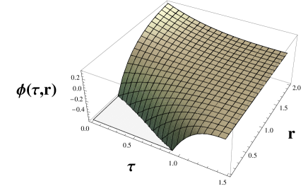
Figure 4: Behavior of the BD scalar field with respect to $\tau$ and r for $\omega=-1$, $w=-\frac{1}{3}$. For the initial energy density, scale factor and proper time we have adopted the values $\rho_{{}_{{}_{0}m}}=1$, $a*=1$ and $t*=0$, respectively.

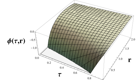
Figure 5: Behavior of the BD scalar field with respect to $\tau$ and r for $\omega=-1$, $w=0$. For the initial energy density, scale factor and proper time we have adopted the values $\rho_{{}_{{}_{0}m}}=1$, $a*=1$ and $t*=0$, respectively.

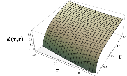
Figure 6: Behavior of the BD scalar field with respect to $\tau$ and r for $\omega=-1$, $w=-\frac{2}{3}$. For the initial energy density, scale factor and proper time we have adopted the values $\rho_{{}_{{}_{0}m}}=2$, $a*=1$ and $t*=0$, respectively.

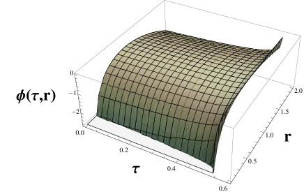
Figure 7: Behavior of the BD scalar field with respect to $\tau$ and r for $\omega=-1$, $w=\frac{1}{3}$. For the initial energy density, scale factor and proper time we have adopted the values $\rho_{{}_{{}_{0}m}}=2$, $a*=1$ and $t*=0$, respectively.

Here $\prime$ denotes partial differentiation with respect to $r$. Solving the above differential equation with a suitable choice of value for $\rho_{{}_{{}_{0}}m}$ one may find the solutions as functions of $\tau$ and $r$. Figs. 4-7 show the behavior of BD scalar field in terms of $\tau$ and $r$ in which the constants of integration have been chosen in such a way that the scalar field blows up near the singularity and get vanished faraway from the collapsing system.

VIII Conclusion and outlook

In this work we have studied the gravitational collapse of the BD scalar field with non-zero potential in the presence of matter fluid. Assuming that the energy density of the BD scalar field behaves as the inverse power law of the scale factor near the singularity, we presented a class of solutions in Brans-Dicke theory in which the naked singularity can be created being accompanied by the violation of the cosmic censorship conjecture. In section III, we found the behavior of BD scalar field as a function of scale factor for the four cases of matter fluid. In section IV, the general expressions of time behavior of the scale factor and singular epoch has been achieved. Having examined the ansatz taken for divergence of the energy density of BD scalar field, Eq. (16), together with the use of Eq. (9) for energy density of matter fluid and by using the concept of expansion parameter, we have shown in section V that the presence of BD scalar field due to the Eq. (14) can affect the formation or otherwise of the trapped surfaces and only for the two cases, $w=-\frac{1}{3}$ and $w=-\frac{2}{3}$, formation of the apparent horizon can be failed and a naked singularity may be generated as the final fate of collapse procedure. But since the absence of an apparent horizon does not necessarily implies the absence of an event horizon, we have computed the Kretschmann scalar in section VI and the result has been plotted in Fig. 1 and Fig. 2 for $w=-\frac{1}{3}$ and $w=-\frac{2}{3}$, respectively. It is seen that this quantity diverges at singular epoch, and then vanishes at late times, a behavior which can be interpreted as the absence of an event horizon and formation of a naked singularity. Also following the work of 33 we have shown at the end of this section that the Vaidya geodesic emerging from the singularity before it evaporates into free space is null.

Beside our work which have only treated exact solutions to gravitational collapse in Brans-Dicke theory, one may find numerical solutions to such a collapse scenario in the literature38 . In 25 ; 29 , the author has developed a new numerical code that solves the gravitational field equations coupled to the matter for evolution of a spherically symmetric configuration of noninteracting particles in Brans-Dicke theory. Using this code, he has shown that Oppenheimer-Snyder collapse in this theory results in black holes rather than naked singularities, at least for $|3+2\omega|\geq 3$, which are identical to those of general relativity in final equilibrium, but are quite different from those of general relativity during dynamical evolution in which they radiate mass. The reason for this behavior is due to the violation of the null energy condition even in vacuum spacetimes with positive values of $\omega$, passing of the apparent horizon of a black hole outside the event horizon, and decreasing the surface area of the event horizon over time. This numerical code enables one to decide on a number of long-standing theoretical questions about collapse in Brans-Dicke theory of gravitation. Also the gravitational collapse of a scalar field with other characteristics and couplings has been discussed in some literature. In 39 , the collapse of a self-similar scalar field has been studied, and it has shown that there exists two classes of solutions which one of them consists of a nonsingular origin in which the scalar field collapses and disperses again. There is a singularity at one point of these solutions which is not observable at a finite radius. The second class of solutions contains both black holes and naked singularities with a critical behavior interpolating between these two extremes. Numerical study of spherically symmetric collapse of a massless scalar field has presented in 40 , where it is shown that the masses of black holes which form satisfy a power law $M_{BH}\propto|p-p^{\ast}|^{\gamma}$. Where $p$ is a parameter which characterizes the strength of initial condition, $p^{\ast}$ is the threshold value and $\gamma\approx 0.37$ is a universal exponent. Also the collapse of a massless scalar field in Brans-Dicke theory has studied both analytically and numerically in 41 and it is shown that for $\omega>-\frac{3}{2}$, a continuous self-similarity continues and that the critical exponent $\gamma$ depends on $\omega$. In 42 , gravitational collapse of a self-interacting (massive) scalar field has been studied both analytically and numerically on a Reissner-Nordsr$\ddot{o}$m background and finally in 43 , one may find some examples of naked singularity formation in gravitational collapse of a scalar field.

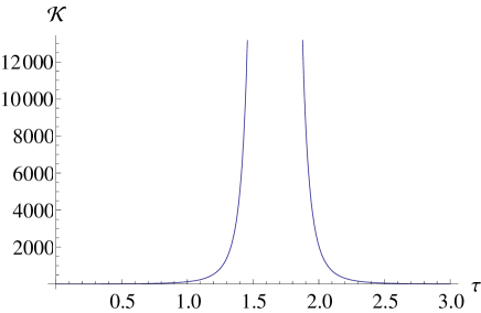
Figure 1: The behavior of Kretschmann scalar (in units of $s^{-4}$) as a function of proper time for $\omega=-1$ and $w=-\frac{1}{3}$. For the initial energy density, scale factor, and proper time we have adopted the values $\rho_{{}_{0m}}=1$, $a^{\ast}=1$, and $\tau^{\ast}=0$, respectively.

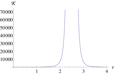
Figure 2: The behavior of Kretschmann scalar (in units of $s^{-4}$) as a function of proper time for $\omega=-1$ and $w=-\frac{2}{3}$. For the initial energy density, scale factor, and proper time we have adopted the values $\rho_{{}_{0m}}=2$, $a^{\ast}=1$, and $\tau^{\ast}=0$, respectively.

Figure 3: Behavior of potential as a function of BD scalar field for $\omega=-1$ and different values of $\rho_{{}_{{}_{0}m}}$ and $w$: $\rho_{{}_{{}_{0}m}}=1$ and $w=0$ (Dotted curve), $\rho_{{}_{{}_{0}m}}=1$ and $w=-\frac{1}{3}$ (Dashed Curve), $\rho_{{}_{{}_{0}m}}=2$ and $w=-\frac{2}{3}$ (Solid Curve), $\rho_{{}_{{}_{0}m}}=2$ and $w=\frac{1}{3}$ (Thick-Dashed Curve).

References

- (1) P. S. Joshi, Gravitational Collapse and Space-Time Singularities, (Cambridge University Press, 2007).
- (2) A. Gromov, Yu. Baryshev, D. Suson and P. Teerikorpi, gr-qc/9906041.
- (3) G. Ann. Soc. Sci Bruxelles A 53 (1933) 51.
- (4) P. S. Joshi and I. H. Dwivedi, Phys. Rev. D 47 (1993) 5357-5369, gr-qc/9303037.
- (5) R. C. Tolman, Proc. Natl. Acad. Sci. USA 20 (1934) 169.
- (6) H. Bondi, Mon. Not. Astron. Soc. 107 (1947) 410.
- (7) A. Ori and T. Piran, Phys. Rev. D 42 (1990) 1068.
- (8) P. Yodzis, H. Seifert and H. zum Hagen, Commun. Math. Phys. 34 (1973) 135.
-
(9)
D. M. Eardly and L. Smarr, Phys. Rev. D 19 (1979) 2239 ;
D. Christodoulou, Commun. Math. Phys. 93 (1984) 171. - (10) W. A. Hiscock, L. G. Williams and D. M. Eardley, Phys. Rev. D 26 (1982) 751.
- (11) R. Goswami and P. S. Joshi, Phys. Rev. D 69 (2004) 027502, gr-qc/ 0310122.
- (12) J. R. Oppenheimer and H. Snyder, Phys. Rev. 56 (1939) 455.
- (13) D. Christodoulou , gr-qc/0805.3880.
- (14) R. Penrose, Rev. Nuovo Cimento 1 (1969) 252.
- (15) F. C. Mena, B. C. Nolan and R. Tavakol, Phys. Rev. D 70 (2004) 084030, gr-qc/0405041.
-
(16)
D. Christodoulou, Ann. of Math. 149 (1999) 183;
J. M. Martin-Garcia and C. Gundlach , Phys. Rev. D 68 (2003) 024011. - (17) K. D. Patil, Phys. Rev. D 67 (2003) 024017.
-
(18)
P. S. Joshi and T. P. Singh, Phys. Rev. D 51 (1995) 6778;
I. H. Dwivedi and P. S. Joshi, Class. Quant. Grav. 14 (1997) 1223;
S. H. Ghate, R. V. Saraykar and K. D. Patil, Pramana, J. Phys. 53 (1999) 253. -
(19)
Y. Kuroda, Prog. Theor. Phys. 72 (1984) 63;
K. Rajagopal and K. Lake, Phys. Rev. D 35 (1987) 1531;
I. H. Dwivedi and P. S. Joshi, Class. Quant. Grav. 6 (1989) 1599;
P. S. Joshi and I. H. Dwivedi, Gen. Relativ. Gravit. 24 (1992) 129;
J. Lemos, Phys. Rev. Lett. 68 (1992) 1447;
K. D. Patil, R.V. Saraykar and S. H. Ghate, Pramana, J. Phys. 52 (1999) 553;
S. G. Ghosh and R. V. Saraykar, Phys. Rev. D 62 (2000) 107502. -
(20)
P. S. Joshi and I. H. Dwivedi, Commun. Math. Phys. 146
(1992) 333;
T. Harada, Phys. Rev. D 58 (1998) 104015. -
(21)
P. Szekeres and V. Lyer, Phys. Rev. D 47
(1993) 4362;
S. Brave, T. P. Singh and L. Witten, Gen. Relativ. Gravit. 32 (2000) 697. -
(22)
S. G. Ghosh and N. Dadhich, Gen. Relativ. Gravit. 35
(2003) 359;
T. Harko and S. K. Cheng, Phys. Lett. A 266 (2000) 249. - (23) P. S. Joshi, R. Goswami and N. Dadhich, gr-qc/0308012.
- (24) P. S. Joshi, N. Dadhich and R. Maartens, Phys. Rev. D 65 (2000) 101501, gr-qc/0109051.
- (25) M. A. Scheel, S. L. Shapiro, and S. A. Teukolsky, gr-qc/9411026.
- (26) P. G. O Freund, Nucl. Phys. B 209 (1982) 146.
- (27) M. B. Green, J. H. Schwarz, and E. Witten, Superstring Theory: 2 (Cambridge: Cambridge Univercity Press, 1987); C. G. Callan, D. Friedan, E. J. Martinek, and M. J. Perry, Nucl. Phys. B 262 (1985) 593.
- (28) D. La and P. J. Steinhardt, Phys. Rev. Lett. 62 (1989) 376; P. J. Steinhardt and F. S. Accetta, Phys. Rev. Lett. 64 (1990) 2740; J. Garcia-Bellido and M. Quiros, Phys. Lett. B 243 (1990) 45.
- (29) M. A. Scheel, S. L. Shapiro, and S. A. Teukolsky, gr-qc/9411025.
- (30) V. Mukhanov, Phisical Foundations of Cosmology, (Cambridge University Press, 2005).
- (31) S. Weinberg, The Quantum Theory of Fields, Vol. 2. Chap 23, Cambridge University Press (1995).
- (32) V. P. Frolov and I. D. Novikov, Black Hole Physics , Copenhagen Edmonton, October 1997.
- (33) R. Goswami and P. S. Joshi, Mod. Phys. Lett. A 22 (2007) 65.
- (34) P. S. Joshi and R. Goswami, Phys. Rev. D 69 (2004) 064027, gr-qc/0206042.
- (35) D. Garfinkle, and G. Comer Duncan, Phys. Rev. D 58 (1998) 064024, gr-qc/9802061.
- (36) P. C. Vaidya, The External Field of a Radiating Star In General Relativity, Curr. Sci. 12 (1943) 183; P. C. Vaidya, The Gravitational Field of a Radiating Star, Proc. Indian Acad. Sci. A. 33 (1951) 264; P. C. Vaidya, Newtonian Time In General Relativity, Nature, 171 (1953) 260.
- (37) P. O. Mazur, and E. Mottola, (2004).’Gravitational vacuum condensate stars’. Proc. Nat. Acad. Sci., 111, 9545.
- (38) K. S. Thorne and J. J. Dykla, Ap. J. 166, L35 (1971); S. W. Hawking, Comm. Math. Phys. 25 (1972) 167; T. Matsuda, Prog. Theo. Phys. 47 (1972) 738.
- (39) P. R. Brady, Phys. Rev. D 51 (1995) 4168.
- (40) M. W. Choptuik, Phys. Rev. Lett. 70 (1992) 9.
- (41) T. Chiba, J. Soda, Prog. Theor. Phys. 96 (1996) 567, gr-qc/9603056.
- (42) S. Hod, T. Piran, Phys, Rev. D 58 (1998) 044018, gr-qc/9801059.
- (43) D. Christodoulou, Annals, Math. 140 (1994) 607.