Properties of stellar generations in Globular Clusters and relations with global parameters

We revise the scenario of the formation of Galactic globular clusters (GCs) by adding the observed detailed chemical composition of their different stellar generations to the set of their global parameters. We exploit the unprecedented set of homogeneous abundances of more than 1200 red giants in 19 clusters, as well as additional data from literature, to give a new definition of bona fide globular clusters, as the stellar aggregates showing the presence of the Na-O anticorrelation. We propose a classification of GCs according to their kinematics and location in the Galaxy in three populations: disk/bulge, inner halo, and outer halo. We find that the luminosity function of globular clusters is fairly independent of their population, suggesting that it is imprinted by the formation mechanism, and only marginally affected by the ensuing evolution. We show that a large fraction of the primordial population should have been lost by the proto-GCs. The extremely low Al abundances found for the primordial population of massive GCs indicate a very fast enrichment process before the formation of the primordial population. We suggest a scenario for the formation of globular clusters including at least three main phases: i) the formation of a precursor population (likely due to the interaction of cosmological structures similar to those that led to the formation of dwarf spheroidals, but residing at smaller galactocentric distances, with the early Galaxy or with other structures), ii) which triggers a large episode of star formation (the primordial population), and iii) the formation of the current GC, mainly within a cooling flow formed by the slow winds of a fraction of the primordial population. The precursor population is very effective in raising the metal content in massive and/or metal-poor (mainly halo) clusters, while its rôle is minor in small and/or metal rich (mainly disk) ones. Finally, we use Principal Component Analysis and multivariate relations to study the phase of metal-enrichment from primordial to second generation. We conclude that most of the chemical signatures of GCs may be ascribed to a few parameters, the most important being metallicity, mass, and age of the cluster. Location within the Galaxy (as described by the kinematics) also plays some rôle, while additional parameters are required to describe their dynamical status.

1 Introduction

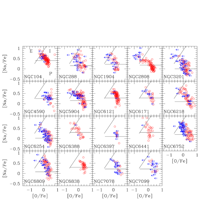
Figure 1: Summary of the Na-O anticorrelation observed in the 19 globular clusters of our sample. Arrows indicate upper limits in oxygen abundances. The two lines in each panel separate the Primordial component (located in the Na-poor/O-rich region), the Na-rich/O-poor Extreme component, and the Intermediate component in-between (called P, E, and I, respectively as indicated only in the first panel). See Sect. 2 for details.

The assembly of the early stellar populations in galaxies is one of the hottest open issues in astronomy. Globular Clusters (GCs) are a major component of these old stellar populations; they are easily detectable and can be studied in some detail even at large distances, providing a potentially powerful link between external galaxies and local stellar populations. A clear comprehension of the mechanisms that led to the formation and evolution of GCs and of the relations existing between GCs and field stars, is a basic requirement to understand how galaxies assemble (see e.g. Bekki et al. 2008). Various authors proposed scenarios for the formation of GCs (Peebles & Dicke 1968; Searle & Zinn 1978; Fall & Rees 1985; Cayrel 1986; Freeman 1990; Brown et al. 1991, 1995; Ashman & Zepf 1992; Murray & Lin 1992; Bromm & Clarke 2002; Kravtsov & Gnedin 2005; Saitoh et al. 2006; Bekki & Chiba 2002, 2007; Bekki et al. 2007; Hasegawa et al. 2009; Marcolini et al. 2009; Hartwick 2009). While very suggestive and intriguing, these scenarios either do not reproduce in a completely convincing way the whole spectrum of observations, or are likely incomplete, describing only part of the sequence of events that lead to GC formation or only a subset of them. We still lack the clear understanding we would need. However, some recent progresses are opening new promising perspectives.

Since almost forty years ago we know that large star-to-star abundance variations for several light elements are present in GCs (see Gratton et al. 2004 for a recent review). Regarded for long time as intriguing abundance “anomalies” restricted to some cluster stars, the observed peculiar chemical composition only recently was explicitly understood as an universal phenomenon in GCs, likely related to their very same nature/origin (Carretta 2006; Carretta et al. 2006, Paper I). The observational pattern of Li, C, N, O, Na, Al, Mg in cluster stars is currently well assessed (see e.g. the review by Gratton et al. 2004), thanks to several important milestones:

• variations for the heavier species (O, Na, Mg, Al) are restricted to the denser cluster environment. The signature for other elements (Li, C, N) may be reproduced by assuming a mixture of primordial composition plus evolutionary changes. The latter are due to two mixing episodes, occurring at the end of the main-sequence (the first dredge-up) and after the bump on the Red Giant Branch (RGB), both in low mass Population II field stars and in their cluster analogues (Charbonnel et al. 1998; Gratton et al. 2000b; Smith and Martell 2003).

• the observed pattern of abundance variations is established in proton-capture reactions of the CNO, NeNa and MgAl chains during H-burning at high temperature (Denisenkov and Denisenkova 1989; Langer et al. 1993);

• the variations are found also among unevolved stars currently on the main-sequence (MS) of GCs (Gratton et al. 2001; Ramirez and Cohen 2002; Carretta et al. 2004; D’Orazi et al. 2010). This unequivocally implies that this composition has been imprinted in the gas by a previous generation of stars. The necessity of this conclusion stems from the fact that low-mass MS stars are unable to reach the high temperatures for the nucleosynthetic chains required to produce the observed inter-relations between the elements (in particular the Mg-Al anticorrelation). This calls for a class of now extinct stars, more massive than the low-mass ones presently evolving in GCs, as the site for the nucleosynthesis.

Unfortunately, we do not know yet what kind of stars produced the pollution. The most popular candidates are either intermediate-mass AGB stars (e.g., D’Antona & Ventura 2007) or very massive, rotating stars (FRMS, e.g., Decressin et al. 2007).

The observed abundance variations are also connected to the helium abundance, since He is the main outcome of H-burning (i.e., Na-rich, O-poor stars should also be He-rich). However, the relation between He abundance variations and the light element abundance pattern may be quite complicate. Multiple main-sequences, attributed to populations with different He fraction Y, have been recently found in some GCs ($\omega$ Cen, NGC 2808, see Bedin et al. 2004 and Piotto et al. 2007, respectively). We have found a clear indication that Na-rich and Na-poor stars in NGC 6218 and NGC 6752 have slightly different RGB-bump luminosities (Carretta et al. 2007b, hereinafter Paper III), as expected from models of cluster sub-populations with different He content (Salaris et al. 2006). In separate papers (Gratton et al. 2010; Bragaglia et al. 2010) we examine in more detail the relation between He and light element abundance variations from evidence based on horizontal branch (HB) and RGB.

In summary, GCs are not exactly a Simple Stellar Population: they must harbour at least two stellar generations, as explained above, clearly distinct by their chemistry. These populations may be separated, provided data of adequate quality are available. The patterns of anticorrelated Na-O, Mg-Al and, partly, C-N, Li-Na (and associated correlations) must be regarded as the fingerprints of these different sub-populations, and may be used to get insights on the early phases of formation and evolution of GCs, which are still obscure. The time scale for the release of matter processed by H-burning at high temperature is of the order of $10^{7}$ yr if it comes from FMRS, and a few times longer if it comes from massive AGB stars. Thus, whatever the candidate producers, the observed patterns were certainly already in place within some $10^{8}$ yr after the start of cluster formation. These processes occurred on time-scales less than 1% of the typical total age of a GC. The dynamical evolution that occurred in the remaining 99% of the cluster lifetime, while likely important, did not completely erase these fingerprints. Their fossil record is still recognisable in the chemical composition of the low mass stars.

To decipher the relevant information we need large and homogeneous data sets, like the one we recently gathered (Carretta et al. 2009a,b). The goal of the present paper is to exploit this wealth of data to discuss the abundance patterns of the different populations within each GC. We will correlate them with global cluster parameters, such as the HB morphology, and structural or orbital parameters. This will allow to better understand which are the main properties of the stellar populations of GCs, hence to get insights into the early phases of their evolution. Using this information as a guide, we will sketch a quite simple scenario for the formation of GCs, which is essentially an updated and expanded version of what proposed thirty years ago by Searle & Zinn (1978). This scenario naturally explains the relation between GCs and other small systems (dwarf Spheroidals), and suggests a connection between GCs and field stars. In fact we propose that the primordial population of GCs might be the main building block of the halo, although other components are likely present.

The present paper is organised as follows. In Sect. 2 we give a brief summary of our previous work, to set the stage for the following discussion. In Sect. 3 we recall some general properties of the GC population and the division in subpopulations; we also present the selection criteria for our sample, discussing possible biases, and the parameters used in the analysis. In Sect. 4 we discuss the properties of the first stellar generation, and we present a scenario for GC formation. In Sect. 5 we consider the second phase of chemical enrichment in GCs, comparing the properties of the second generation with those of the primordial one and presenting a number of interesting correlations. Finally, in Sect. 6, we discuss in a more general way the correlations with global GC parameters and give a summary and conclusions. In the Appendix, we present a new classification of all Galactic GCs, dividing them into disk/bulge, inner halo, and outer halo ones on a kinematical basis; we also list their metallicities on the scale defined in Carretta et al. (2009c), their ages, re-determined from literature using these metallicities, and a compilation of [$\alpha$/Fe] values, that are used throughout the paper.

2 Synopsis of previous results

We give here a summary of results from our project “Na-O anticorrelation and HB” (Carretta et al. 2006) propaedeutic to the present discussion.

Up to a few years ago, obtaining adequate high resolution spectroscopic data sets was painstaking, since stars had to be observed one-by-one. Thanks to the efforts of many researchers, mainly of the Lick-Texas group, spectra of some 200 stars in a dozen GCs were gathered using tens of nights over several years (see the reviews by Kraft 1994, Sneden 2000 and references therein). In the last few years, we used the spectacular data collecting capability offered by the FLAMES multi-object spectrograph at the ESO VLT to secure spectra for more than 1400 giant stars, distributed over about 12% of all known GCs. With the increase of an order of magnitude in available data, the paradigm has changed. We now understand that the observed anticorrelations are not indicative of “anomalies”, rather we are dealing with the normal chemical evolution of GCs.

Our survey has already been amply described elsewhere. Results for the first five GCs have been presented in a series of papers (Papers I through VI: Carretta et al. 2006, 2007a,b,c; Gratton et al. 2006, 2007), while the remaining clusters are analysed in Carretta et al. (2009a,b: Paper VII and VIII). In Fig. 1 we show a collage of the Na-O anticorrelations observed in all 19 clusters in our sample. Solid lines separate the Primordial, Intermediate and Extreme populations, whose concept is introduced and defined in Paper VII and recalled briefly below.

Very shortly, we obtained GIRAFFE spectra (at R$\simeq$20000, comprising the Na i 568.2-568.8 nm, 615.4-6.0 nm and [O i] 630 nm lines) of about 100 stars per cluster. At the same time, we also collected UVES spectra (at R$\simeq$40000, covering the 480-680 nm region, and providing information about Mg, Al, and Si, in addition to O and Na) of about 10 stars (on average) per cluster. We homogeneously determined the atmospheric parameters for these stars using visual and near-IR photometry and the relations in Alonso et al. (1999, 2001). We measured Fe, O, and Na abundances for more than 2000 stars (more than 1200 cluster members with $both$ O and Na detected), putting together the largest sample of this kind ever collected.

This large statistics, both in the number of clusters and in stars per cluster, allowed us to recognise that the amount of the abundance variations among different clusters is related in a not trivial way to global cluster parameters (Carretta 2006; Carretta et al. 2007a; 2009a, Paper VII: GIRAFFE data; 2009b, Paper VIII: UVES data). The GCs are dominated by the second (polluted) generation of stars, the fraction of primordial stars being roughly correlated with cluster luminosity. The Na-O anticorrelation has not only different extension, but also different $shape$, in different clusters, depending on cluster luminosity and metallicity. The Mg-Al anticorrelation is sometimes absent, this occurring in low-luminosity clusters. All these are clear indications that the polluters’ properties change from cluster to cluster and that this change is apparently driven by the cluster luminosity and metallicity.

Carretta (2006) suggested to use the Interquartile Range (IQR, the difference between the upper quartile and the lower quartile, see e.g. Tukey 1977) of the [O/Na] ratio as a quantitative measure of the extension of the Na-O anticorrelation. The IQR is useful because it is less influenced by extreme values, it refers to the range of the middle 50% of the values and it is less subject to sampling fluctuations in highly skewed distributions. Statistically robust IQR values require large enough samples of stars. Our project was designed to obtain Na and O abundances for a large number of RGB stars in each cluster, typically 100 stars per cluster, although in some cases only a much smaller sample of stars could be used. The number of stars actually measured in each cluster depends on the richness of population, metallicity, $S/N$ ratio, and in some cases on field stars contamination (like for the bulge clusters NGC 6388 and NGC 6441, or the disk clusters NGC 6171 and NGC 6838). The smallest sample (16 stars with both Na and O) is for NGC 6397, the largest (115 stars) is for 47 Tuc (NGC 104).

In Paper VII we defined three population components in each cluster: the first generation stars, and two groups of second generation stars. The lines separating the three components are shown in Fig. 1. The primordial P component includes stars between the minimum [Na/Fe] observed and [Na/Fe]${}_{min}+4\sigma$ (see Paper VII). These stars are defined as first generation objects since they show the same pattern of high O and low Na typical of galactic field stars of similar metallicity, with the characteristic signature of core-collapse SNe. Since the yields of Na are metallicity-dependent (e.g.,Wheeler et al. 1989), the limit for the P component varies as a function of [Fe/H], as evident in Fig. 1. The separation between the two sub-components of second generation stars (the intermediate I stars and the extreme E stars) is somewhat more arbitrary. On the basis of the [O/Na] distributions in our clusters, they were defined in Paper VII as those stars with [O/Na] ratios larger or smaller than -0.9 dex, respectively.

Computing the fraction of stars in each component, we found that:

• the Extreme 2nd generation is not present in all GCs;

• the Intermediate 2nd generation constitutes the bulk (50-70%) of stars in a GC;

• the Primordial population is present in all GCs (at about the 30% level).

D’Antona and Caloi (2008) used the HB morphology to derive the fraction of stars in two generations in GCs. They made a claim that some clusters (including NGC 6397) could presently host exclusively second generation stars, having completely lost the first generation ones. However, our abundance analysis, in comparison with field stars, does not support that hypothesis. In Fig. 2 we show the distribution of [Na/Fe] in field stars with metallicity centred on the mean [Fe/H] value for NGC 6397. Filled circles are our RGB stars in NGC 6397 with both Na and O measurements (Paper VII and Paper VIII), separated in P and I components using our definition. To be very conservative, in Paper VII we attributed to each of the three populations only stars with both elements measured. However, the separation between first and second generation stars (between P and I components) only requires the knowledge of Na abundances. In Fig. 2 the much more numerous stars in NGC 6397 with Na detections are plotted as open star symbols. A good fraction of them fall in the region populated by the Primordial component and by normal field halo stars, unpolluted by ejecta processed in H-burning. Hence, we confirm that in all GCs analysed a primordial component of first generation stars is still observable at present.

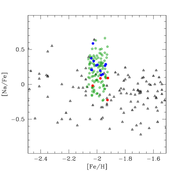
Figure 2: [Na/Fe] ratios as a function of the metallicity [Fe/H] in a range centred on the average metal abundance of NGC 6397. Filled triangles in grey-tones are field stars from Gratton et al. (2003a) and the compilation by Venn et al. (2004). Filled circles are stars in NGC 6397 with determinations of both O and Na (red: P component, blue: I component). Empty (green) star symbols are stars in NGC 6397 with only Na abundances derived.

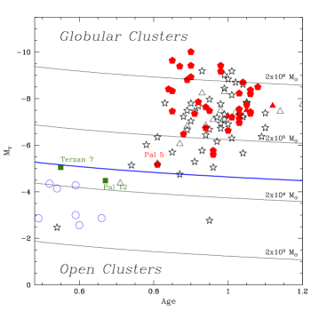
Figure 3: Relative Age parameter vs absolute magnitude $M_{V}$ for globular and old open clusters (see Appendix for details). Red filled pentagons and triangles are GCs where Na-O anticorrelation has been observed, in the Milky Way or the LMC respectively; green squares are clusters which do not show evidence for O-Na anticorrelation, both members of Sagittarius dSph, either of the main body (Terzan 7) or the stream (Pal 12). Open stars and triangles mark clusters for which not enough data is available, in the Milky Way or the LMC respectively. Finally, open circles are old open clusters (data from Lata et al. 2002). Superimposed are lines of constant mass (light solid lines, see Bellazzini et al. 2008a). The heavy blue solid line (at a mass of $4\times 10^{4}\leavevmode\nobreak\ M_{\odot}$) is the proposed separation between globular and open clusters.

3 Clusters and parameters selection

3.1 Definition of globular clusters

In this paper we intend to bring together the chemical properties derived from our in-depth study of various stellar populations in GCs with many other global observables. Moreover, we present a scenario for the formation of GCs in the more general context of the relationship between the Milky Way and its satellites. Thus, before entering into the discussion, we recall a few properties of the parent population of GCs that are of direct interest here.

The first point we would like to make concerns the operative definition of bona fide GC. The distinction between globular and other clusters (e.g., open clusters) is not well drawn, and it is ambiguous in particular for the populous clusters that are numerous in the Magellanic Clouds. To better clarify this point, we plot in Figure 3 ages and absolute magnitudes for the clusters listed in the database by Harris (1996, and web updates). This list includes 146 GCs. Seven of these GCs are actually thought to be members of the Sagittarius dwarf galaxy (see van den Bergh & Mackey 2004, and references therein). To this sample, we add GCs in other satellites of the Milky Way: 16 GCs in the Large magellanic Cloud (LMC), 8 in the Small Magellanic Cloud (SMC) and 5 in the Fornax dwarf Spheroidal, dSph). Data for all these GCs are detailed in the Appendix. Age data are actually available for slightly more than half of the sample. We also add for a few old open clusters (NGC 188, NGC 6791, Collinder 261, NGC 1193, Berkeley 31, and Berkeley 39: data from Lata et al. 2002), that fall within the limits of the plot. From this figure, there is a clear overlap between open clusters and objects from the list of GCs at the faint end of the sequence. We used filled red pentagons for those GCs where the Na-O anticorrelation has been found. One of the filled green squares indicates Terzan 7, where no spread in O abundances has been found in the (only) seven stars observed by Sbordone et al. (2007), and may then be the most massive cluster observed insofar without the Na-O anticorrelation. The other one is Pal 12, where Cohen (2004) finds very uniform O and Na abundances, but only on four stars. Finally, open symbols are for all remaining GCs, for which current data are not adequate to state if a Na-O anticorrelation exists or not. Similar data are scarce for open clusters (see Gratton 2007). However, de Silva et al. (2009) compiled data for various old open clusters, finding no evidence for a Na-O anticorrelation, and Martell & Smith (2009) did not find any evidence for CN variation among giants in three open clusters (including NGC 188). This diagram indicates that the Na-O and related anticorrelations have been observed in all old clusters with $M_{V}<-5.1$ (which roughly corresponds to a mass of $\sim 4\times 10^{4}\leavevmode\nobreak\ M_{\odot}$ for old populations), including the vast majority of galactic GCs, and almost all the objects with a relative age parameter $>0.8$. We then propose to identify the GCs with those clusters where there is a Na-O anticorrelation. As we will see in Sect. 4.1, this identification corresponds to a formation scenario which clearly separates GCs from other clusters. Operatively, we might also define GCs either as the old clusters (age larger than 5 Gyr) with a $M_{V}<-5.1$, or those with relative age parameter $>0.8$. These definitions essentially include the same list of objects, at least in the Milky Way and its satellites.

At the other mass limit for the GC population, the similarity between GCs and nuclei of dwarf galaxies has been pointed out by many authors (see e.g. Freeman 1990; Böker 2008; Georgiev et al. 2009). Those nuclei or nuclear star clusters of dwarf galaxies that can be studied in good detail (like M 54 for the Sagittarius galaxy) essentially share the whole pattern of properties with GCs (see e.g. Bellazzini et al. 2008b; Georgiev et al. 2009, Carretta et al. 2010), although they may have large spreads in Fe abundances, not observed in GCs. This occurrence suggests that also $\omega$ Cen was in the past (in) the nucleus of a galaxy.

3.2 Our sample of GCs

Ideally, we should have derived detailed chemical data for the whole parent population. However, this would have required too much observing time and we analysed only a representative subset of clusters (representing about 12% of the total sample). The selection procedure was as follows. We started from the whole sample of galactic GCs, as listed by Harris (1996). We then divided clusters in different groups, according to the morphology of the HB. For each group, we selected the two-four rich ($M_{V}<-5$) clusters, accessible from Paranal ($\delta<+20\degr$), with the smallest apparent distance modulus; however we did not consider some clusters that have quite large differential reddening (like M 22: Ivans et al. 2004). The selected clusters were: Red HB clusters: NGC 104=47 Tuc, NGC 6838=M 71, NGC 6171=M 107; Oosterhoff I clusters: NGC 6121=M 4, NGC 3201, NGC 5904=M 5; Blue Horizontal Branch clusters: NGC 6752, NGC 6218=M 12, NGC 6254=M 10, NGC 288, NGC 1904=M 79; clusters with blue, short HB’s: NGC 6397, NGC 6809=M 55; Oosterhoff II clusters: NGC 7099=M 30, NGC 4590=M 68, NGC 7078=M 15; Clusters with very extended/bimodal distribution of stars on the HB: NGC 2808, NGC 6441, NGC 6388. Hence, within each different class of HB morphology, the sample is essentially distance limited. On the other hand, this is not true for the whole sample, because the adopted limits depend on the morphological classes and reddening (so that clusters projected close to the Galactic plane are under-represented). However, for most classes of HB’s, the limit is quite uniform at about (m-M)${}_{V}<14.5-15.5$, that is $\sim 10$ kpc from the Sun. We needed to sample a larger volume ((m-M)${}_{V}<16.5$) to include GCs with very extended/bimodal distribution of stars on the HB, since these clusters are rare. Due to these choices, GCs with very extended blue HB are over-represented in our sample (42% of the total).

3.3 The Galactic GC sample

To correctly explore the relations between the chemistry of different stellar generations and global GC properties, it is important to assess to what cluster population our programme GCs belong. Zinn (1985) demonstrated that Milky Way GCs can be divided into two main groups: disk (or bulge) GCs, and halo GCs. This separation was done according to the metal abundance only (with the limit at [Fe/H]$=-0.8$ dex). These two groups correspond to the main peaks of the metallicity distribution of GCs, but they can also be clearly distinguished from other properties (location in the Galaxy, kinematics, etc.). According to Searle & Zinn (1978), halo GCs result from the evolution of individual fragments, while disk clusters likely formed within the dissipational collapse. Hence this distinction is likely to play an important rôle in defining the characteristics of GCs, and in particular of their primordial population.

Further refinements (e.g., van den Bergh & Mackey 2004, Lee et al. 2007) along Zinn’s line of thought were done by using the HB morphology which, however, is one of the features of GCs we intend to explain. In the following therefore, we will adopt a combination of location in the Galaxy and kinematics criteria to separate disk clusters from the halo ones. Full details are given in the Appendix. Briefly, using the Harris (1996) catalogue, we have first classified as outer halo GCs the ones currently located at distances greater than 15 kpc (Carollo et al. 2008) from the Galactic centre; clusters with Galactocentric distance less than 3.5 kpc were instead considered as bulge GCs. To separate the inner halo clusters from the disk ones, we used the rotational velocity around the Galactic centre by Dinescu et al. (1999) and Casetti-Dinescu et al. (2007) whenever possible. When this datum was not available, we used the differences between the observed radial velocity (corrected to the LSR) and the one expected from the Galactic rotation curve (see Clemens 1985). In the Appendix we provide the disk/inner halo/outer halo classification for each cluster listed in the Harris catalogue. Finally, we consider GCs in the LMC, SMC, and in dSph’s (Sagittarius and Fornax) as separate groups.

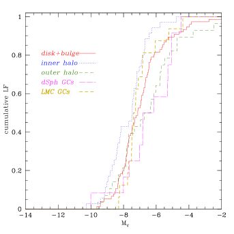
Figure 4: Cumulative luminosity functions of different groups of Galactic GCs (from the Harris 1996 catalogue) according to our present classification criteria, and of GCs in dwarf spheroidals (from van den Bergh and Mackey 2004; see Appendix for references on Fornax an LMC clusters). The red solid line indicates disk/bulge clusters, the blue dotted line the inner halo clusters, the dashed green line clusters in the outer halo, magenta dashed-dotted line is for clusters in dSphs, and the green-gold long dashed line for GCs in LMC.

The procedure to select the programme sample, described in Sect. 3.2, results in a potential selection bias as a function of the distance. This shows up in a correlation between cluster present-day mass (as represented by the proxy of cluster total absolute visual magnitude, $M_{V}$) and distance modulus: in our sample more massive GCs are typically the most distant ones. This correlation is at odds with the total sample of GCs in the Harris (1996) catalogue. However, since all programme GCs but one (NGC 1904, with $R_{GC}=18.8$ kpc) are within 15 kpc from the Galactic centre they belong either to the disk or to the inner halo. Within this sub-sample, there is a correlation of $M_{V}$ with Galactocentric distance similar to that noticed in our sample. Hence, we will assume that our sample is representative of the properties of the disk and inner halo (but not of the outer halo) GCs, and will neglect the possible bias with luminosity.

Other properties of the parent population of Galactic GCs relevant for our discussion are the masses (luminosities) and the metallicities of the disk and inner halo GCs. These are two of the main parameters driving most of the observed properties of GCs, as we will confirm later, and are worth a few more words.

Inner and outer halo clusters have clearly distinct luminosity functions (LF), as illustrated by Fig. 4. Small clusters (M${}_{\rm V}>$-6) only exist in the outer halo, where they make up half of the total. A Kolmogorov-Smirnov test returns a 1% probability that inner and outer halo LF were extracted from the same population. Of course, this difference can be at least in part attributed to the destruction mechanisms, which are more efficient for clusters closer to the centre of the Galaxy. However, other mechanisms can also be considered. In fact, all young clusters (Age parameter $<0.8$) reside in the outer halo, and they are all faint ($M_{V}>-6.5$), overlapping open clusters in the $M_{V}$/age distribution (Fig.3). If we limit to old clusters (Age parameter $>0.82$, essentially adopting the same definition of GC considered in Sect. 3.1), there is no clear difference between the LF of inner halo or disk and that of outer halo clusters (Kolmogorov-Smirnov tests for the distribution of the GCs with age parameter available return significance of 16 and 32%, respectively).

Also the comparison between the LFs of disk and inner halo GCs is worth more attention. Again, we naively expected that destruction mechanisms should be more effective for disk clusters than for the inner halo ones. In this case the LF for inner halo clusters should have a fraction of small mass clusters intermediate between those observed in the outer halo and in the disk. However, while only 19% (4%) of the inner halo GCs have $M_{V}>-7$ ($M_{V}>-6$), this percentage is 41% (15%) for disk clusters. There are very few inner halo counterparts of the very frequent small disk clusters like M 71 and NGC 6397. Since such clusters are more easily destroyed in the disk than in the inner halo, this suggests a different original mass distribution between the disk and the inner halo (see also Fraix-Burnet et al. 2009, who attempted a multi-parametric classification of GCs, different from ours and leading to different conclusions about the properties of the different cluster populations, see the Appendix for further details).

All this suggests that the main difference between disk, inner and outer halo clusters might be related to their formation (absence of young, small clusters in the inner halo) more than to the destruction efficiency, which is however very important for small clusters. This goes against a diffuse opinion, i.e., that we are now seeing only those GCs which occupied the survival zone of parameters; however, the notion that GCs can be formed only in a limited range of parameters is not new, see for instance Caputo & Castellani (1984).

It is also interesting to note that the luminosity function of the outer halo GCs is similar to that of GCs in dSph’s (see Fig.4): a Kolmogorov-Smirnov test gives a chance (73%) that they were drawn from the same parent population. This might depend on the fact that clusters in the outer halo and dSph shared similar environments at birth.

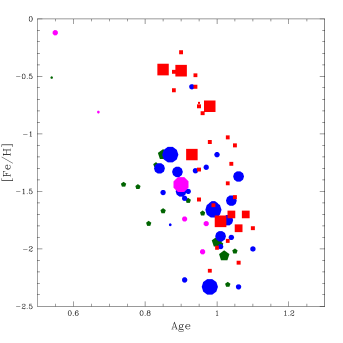
Figure 5: Age-metallicity relation for different groups of globular clusters: outer halo clusters (green pentagons), inner halo clusters (blue circles), disk/bulge clusters (red squares). Magenta circles are GCs associated to dSphs. Different symbol sizes are used for clusters of different luminosity.

Disk and halo GCs differ also in other important characteristics. Obviously, the inner halo/outer halo GCs are on average more metal poor than the disk ones (see Appendix). Furthermore, they seem to obey to different age metallicity relations: metallicity increased slower in the inner halo than in the disk, and even slower in the outer halo, see Fig. 5. The age estimates were obtained as described in the Appendix. Practically all disk/bulge GCs with [Fe/H]$<-1$ are very old, while most of the inner halo GCs of intermediate metallicity ($-2<$[Fe/H]$<-1$) have relative ages in the range 0.8-0.9, i.e., they are about 2 Gyr younger than disk GCs with the same metallicity. If the age/metallicity calibration is correct, after 2 Gyr from the Big Bang, the central region of the Milky Way was enriched to [Fe/H]$\sim-0.4$ (and [$\alpha$/H]$\sim 0$), while the inner halo metallicity was still very low.

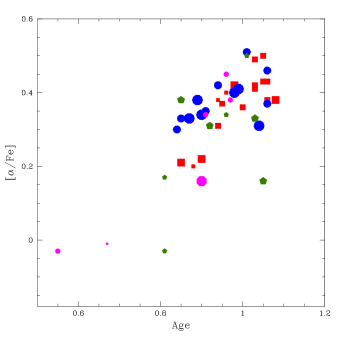
Figure 6: Relation between age and excess of $\alpha-$elements for different groups of globular clusters (the meaning of symbols is as in Fig. 5). [$\alpha$/Fe] values come from our compilation of literature data (see Appendix). Different symbol sizes are used for clusters of different luminosity.

Finally, disk and inner halo GCs may differ in their element-to-element abundance ratios, as suggested by the analysis by Lee & Carney (2002). In part, this can be attributed to an age effect (see Fig. 6); however, age cannot be the only explanation. This is shown by the close comparison between M 4 and M 5 (NGC 6121 and NGC 5904), performed by Ivans et al. (2001), which is fully confirmed by our analysis (Carretta et al. 2009b). These GCs are both inner halo clusters according to our classification, although M 5 has much more extreme kinematics, and it is also likely younger by more than 1 Gyr. M 5 has a smaller excess of $\alpha-$elements, and seems to be also deficient in nuclei produced by $s-$process nucleosynthesys (Ivans et al. 2001; Yong et al. 2008). If confirmed, these two facts might at first look contradictory, since a lower excess of $\alpha-$elements is usually attributed to a prolonged star formation, allowing significant contribution by type Ia SNe. However, such a long phase of star formation should also allow the contribution by the intermediate and small mass AGB stars, which efficiently produce $s-$elements. In the next sections, we will re-examine this point using our extensive database, and find a solution to this conundrum.

3.4 Cluster Parameters considered in the analysis

Our choice was driven by the aim of sampling the full parameter space of GCs and to derive relations between the properties of different stellar generations in GCs and global parameters.

Tab. 1 lists the 19 GCs in our programme set and gives structural and orbital parameters taken from literature. We considered the following parameters, mostly from Harris (1996):

• the apparent visual distance modulus, $(m-M)_{V}$

• the reddening, E(B-V)

• the Galactocentric distance, R_GC

• the total absolute visual magnitude, M_V

• the HB ratio, HBR, that is the fraction of blue and red HB stars over the total, as $(B-R)/(B+V+R)$

• the metallicity, [Fe/H] from our Paper VIII

• the cluster ellipticity, $ell$

• the concentration, $c$

• the tidal radius, $r_{t}$ (in pc, from Mackey and van den Bergh 2005)

• the half light radius, $r_{h}$ (in pc, from Mackey and van den Bergh 2005)

We considered the following parameters related to the Galactic orbit (from Dinescu et al. 1999; Casetti-Dinescu et al. 2007):

• the total energy of orbit, E_tot

• the period of the Galactic orbit, P

• the apogalactic distance, R_apo

• the perigalactic distance, R_per

• the maximum distance from the plan, z_max

• the eccentricity of the orbit, $ecc$

• the inclination angle of the orbit, $\psi$

• the rotational velocity, $\Theta$

These orbital parameters are mean values averaged over a large number of orbits. Hence, they represent a way to gain knowledge on the birthplace of clusters and on the conditions existing at their formation epoch, and where most of their lifetime is spent in the Galaxy. Instantaneous quantities, such as the present Galactocentric distance of a GC, may be much less informative. Unfortunately, no orbital parameters have been determined yet for the two most massive clusters in our sample, NGC 6388 and NGC 6441.

In addition, we considered the relative age parameter, mostly re-determined from Marin-Franch et al. (2009) and De Angeli et al. (2005) as described in the Appendix.

Table 1: Properties of the 19 GCs in our sample.

NGC	other	(m-M)${}_{V}^{1}$	$E(B-V)^{1}$	R${}_{GC}^{1}$	Z1	M${}_{V,tot}^{1}$	HBR1	[Fe/H]1	ell1	$c^{1}$	$r_{h}^{1}$	$r_{t}^{1}$
104	47Tuc	13.32	0.04	7.4	-3.2	-9.42	-0.99	-0.768	0.09	2.03	2.79	42.86
288		14.64	0.03	12.0	-8.8	-6.74	0.98	-1.305		0.96	2.22	12.94
1904	M79	15.53	0.01	18.8	-6.3	-7.86	0.89	-1.579	0.01	1.72	0.80	8.34
2808		15.59	0.22	11.1	-1.9	-9.39	-0.49	-1.151	0.12	1.77	0.76	15.55
3201		14.17	0.23	8.9	0.8	-7.46	0.08	-1.512	0.12	1.30	2.68	28.45
4590	M68	15.14	0.05	10.1	6.0	-7.35	0.17	-2.265	0.05	1.64	1.55	30.34
5904	M5	14.41	0.03	6.2	5.4	-8.81	0.31	-1.340	0.14	1.83	2.11	28.40
6121	M4	12.78	0.36	5.9	0.6	-7.20	-0.06	-1.168	0.00	1.59	3.65	32.49
6171	M107	15.01	0.33	3.3	2.5	-7.13	-0.73	-1.033	0.02	1.51	2.70	17.44
6218	M12	13.97	0.19	4.5	2.2	-7.32	0.97	-1.330	0.04	1.39	2.16	17.60
6254	M10	14.03	0.28	4.6	1.7	-7.48	0.98	-1.575	0.00	1.40	1.81	21.48
6388		16.49	0.37	3.2	-1.2	-9.42	-0.65	-0.441	0.01	1.70	0.67	6.21
6397		12.31	0.18	6.0	-0.5	-6.63	0.98	-1.988	0.07	2.50	2.33	15.81
6441		16.33	0.47	3.9	-1.0	-9.64	-0.76	-0.430	0.02	1.85	0.64	8.00
6752		13.08	0.04	5.2	-1.7	-7.73	1.00	-1.555	0.04	2.50	2.34	55.34
6809	M55	13.82	0.08	3.9	-2.1	-7.55	0.87	-1.934	0.02	0.76	2.89	16.28
6838	M71	13.70	0.25	6.7	-0.3	-5.60	-1.00	-0.832	0.00	1.15	1.65	8.96
7078	M15	15.31	0.10	10.4	-4.7	-9.17	0.67	-2.320	0.05	2.50	1.06	21.50
7099	M30	14.57	0.03	7.1	-5.9	-7.43	0.89	-2.344	0.01	2.50	1.15	18.34
NGC	other	E${}_{tot}^{2}$	P2	R${}_{apo}^{2}$	R${}_{per}^{2}$	z${}_{\rm max}^{2}$	ecc2	$\psi^{2}$	$\Theta$	age3
104	47Tuc	-872	190	7.3	5.2	3.1	0.17	29	161	0.95
288		-787	224	11.2	1.7	5.8	0.74	44	-27	0.90
1904	M79	-526	388	19.9	4.2	6.2	0.65	28	83	0.89
2808		-770	240	12.3	2.6	3.8	0.65	18	74	0.83
3201		-430	461	22.1	9.0	5.1	0.42	18	-301	0.82
4590	M68	-396	504	24.4	8.6	9.1	0.48	30	300	0.94
5904	M5	-289	722	35.4	2.5	18.3	0.87	33	115	0.85
6121	M4	-1121	116	5.9	0.6	1.5	0.80	23	24	0.97
6171	M107	-1198	87	3.5	2.3	2.1	0.21	44	151	0.99
6218	M12	-1063	125	5.3	2.6	2.3	0.34	33	130	0.99
6254	M10	-1053	128	4.9	3.4	2.4	0.19	33	149	0.92
6388										0.87
6397		-1017	143	6.3	3.1	1.5	0.34	18	133	0.99
6441										0.83
6752		-977	156	5.6	4.8	1.6	0.08	18	199	1.02
6809	M55	-1038	122	5.8	1.9	3.7	0.51	56	55	1.02
6838	M71	-957	165	6.7	4.8	0.3	0.17	3	180	0.94
7078	M15	-752	242	10.3	5.4	4.9	0.32	36	128	1.01
7099	M30	-937	159	6.9	3.0	4.4	0.39	52	-104	1.08

• global parameters, from Harris (1996), except [Fe/H], which is from UVES spectra (Paper VIII) and the HBR for NGC 6388, NGC 6441 calculated from Busso et al. (2007)

• orbital parameters, from Dinescu et al. (1999), Casetti-Dinescu et al. (2007). Units are: $10^{2}km^{2}sec^{-2}$ (E_tot), 10⁶ yr (P), kpc (R_apo, R_per, z_max), degrees ($\psi$), km s^-1 ($\Theta$)

• relative age (see Appendix).

Table 2: Quantities for the same GCs, derived by our works

NGC	log T${}_{\rm eff}^{\rm max}$	IQR[Na/O]1	P2	I2	E2	$\langle[\alpha/{\rm Fe}]\rangle^{3}$	[(Mg+Al+Si)	[Mg/Fe]${}_{max}^{6}$	[Mg/Fe]${}_{min}^{6}$	[Si/Fe]${}_{min}^{6}$	[Si/Fe]${}_{max}^{6}$
	(HB)						/Fe]6
104	3.7564	0.472	27	69	4	0.42	0.46	0.60	+0.47	0.35	0.43
288	4.2215	0.776	33	61	6	0.42	0.41	0.55	+0.41	0.30	0.41
1904	4.3524	0.759	40	50	10	0.31	0.31	0.40	+0.16	0.25	0.34
2808	4.5684	0.999	50	32	18	0.33	0.29	0.42	$-$0.30	0.22	0.38
3201	4.0794	0.634	35	56	9	0.33	0.32	0.45	+0.27	0.25	0.41
4590	4.0414	0.372	40	60	0	0.35	0.40	0.48	+0.28	0.30	0.48
5904	4.1764	0.741	27	66	7	0.38	0.36	0.55	+0.31	0.21	0.39
6121	3.9685	0.373	30	70	0	0.51	0.54	0.65	+0.50	0.45	0.64
6171	3.8754	0.522	33	60	7	0.49	0.53	0.60	+0.46	0.45	0.63
6218	4.2174	0.863	24	73	3	0.41	0.43	0.60	+0.46	0.22	0.43
6254	4.4005	0.565	38	60	2	0.37	0.37	0.58	+0.33	0.18	0.36
6388	4.2554	0.795	41	41	19	0.22	0.30	0.40	+0.16	0.20	0.46
6397	3.9784	0.274	25	75	0	0.36		0.55	+0.40	0.25	0.43
6441	4.2304	0.660	38	48	14	0.21	0.34	0.45	+0.20	0.15	0.45
6752	4.4715	0.772	27	71	2	0.43	0.44	0.60	+0.36	0.28	0.49
6809	4.1535	0.725	20	77	2	0.42	0.43	0.60	+0.18	0.30	0.51
6838	3.7634	0.257	28	72	0	0.40	0.44	0.60	+0.39	0.30	0.51
7078	4.4774	0.501	39	61	0	0.40	0.46	0.68	$-$0.01	0.28	0.60
7099	4.0794	0.607	41	55	3	0.37	0.44	0.60	+0.44	0.20	0.45

• IQR([Na/O]) comprises stars with GIRAFFE and UVES data

• P,I,E are fraction of stars of Primordial, Intermediate, Extreme populations from Paper VII

• [$\alpha$/Fe] is the average of [Mg/Fe]_max, [Si/Fe]_min and [Ca/Fe]

• log T${}_{\rm eff}^{\rm max}$(HB) taken from Recio-Blanco et al. (2006)

• log T${}_{\rm eff}^{\rm max}$(HB) derived in the present work (see Section 5.2)

• from Paper VIII

In Tab. LABEL:t:tabnoi we report a few of the parameters derived by our works, related to the chemistry of first and second generation stars in GCs and their link with primordial abundances existing at the epoch of their formation. Other parameters derived, but not listed, in Paper VII and VIII, are also given in this Table.

Among these, we considered parameters related to the chemistry of first generation stars:

• the maximum O abundance, [O/Fe]_max

• the minimum Na abundance, [Na/Fe]_min

• the maximum Mg abundance, [Mg/Fe]_max

• the minimum Al abundance, [Al/Fe]_min

• the minimum Si abundance, [Si/Fe]_min

• the total Mg+Al+Si content, where the average is done in number, not in logarithm, [(Mg+Al+Si)/Fe]

• the overabundance of $\alpha-$elements, [$\alpha$/Fe], as given by the average of [Mg/Fe]_max, [Si/Fe]_min and [Ca/Fe] (see Sect. 4.2.1 for an explanation of the choice).

Coupled with [Fe/H], these parameters essentially describe the starting composition of the proto-GCs. The elements here considered are mainly produced by core collapse SNe, with some contribution by thermonuclear SNe for what concerns Fe (and marginally Si). The sum Mg+Al+Si essentially describes the primordial abundance of elements with $24<{\rm A}<28$ for two reasons. First, this quantity does not differ between different stellar generations in a cluster. As an example, in NGC 2808, the average value of the ratio [(Mg+Al+Si)/Fe] is $+0.29\pm 0.01$ dex (rms=0.03 dex) for the 9 stars in the P, I components and $+0.28\pm 0.02$ dex (rms=0.04 dex) for the three stars with sub-solar Mg values, belonging to the E component (see Paper VIII, Al was measured only on UVES spectra). Second, the only way to get significant modifications of this primordial ratio is to produce the dominant species ²⁴Mg or ²⁸Si from SN nucleosynthesis. Hence, in the following we will adopt this ratio essentially as another indicator of the $\alpha-$element level in a cluster..

Parameters related to the internal chemical evolution within the clusters are:

• the minimum O abundance, [O/Fe]_min

• the maximum Na abundance, [Na/Fe]_max

• the minimum Mg abundance, [Mg/Fe]_min

• the maximum Al abundance, [Al/Fe]_max

• the maximum Si abundance, [Si/Fe]_max

• the relative fraction of stars in Primordial (P), Intermediate (I), and Extreme (E) groups

• the interquartile range of the [O/Na] ratio, IQR[O/Na]

Minimum and maximum abundances of different elements were estimated as discussed in Papers VII and VIII, using a dilution model that reproduces the run of the observed Na-O, Mg-Al and Mg-Si anticorrelations in GCs.

Finally, to explore the connection between chemical patterns of light elements, He abundances, and HB morphology we considered the maximum temperature $\log T_{\rm eff}^{\rm max}(HB)$ reached on the blue tail of the HB (taken by Recio-Blanco et al. 2006 or computed by us for programme clusters not listed in that study).

4 First generation stars, primordial abundances, and scenarios for cluster formation

The chemical pattern in GC first generation stars is strictly related to the pre-enrichment established in the precursors of GCs, an issue for which we only have, at the very best, indirect evidence. In this section we discuss what evidence can be obtained from our data on the scenario of formation of GCs.

4.1 The masses of proto-GCs and the relation between the primordial population of GCs and the field

The scenario we are devising assumes that practically $all$ globular clusters started their evolution as large cosmological fragments. To put cluster formation in a broader context, we try to establish the order of magnitude of the mass involved in cluster formation, and discuss the possible link between GCs and field stars. Using different lines of thought, several authors (Larson 1987; Suntzeff & Kraft 1996; Decressin et al. 2008; D’Ercole et al. 2008) suggested that present-day GCs are only a fraction (likely small) of the original structures where they originated. Large amounts of mass should be lost by proto-clusters during the early phases of formation (a few $10^{7}$ yr), mainly for two reasons. First, the efficiency of transformation of gas into stars is unlikely to be larger than 50%, and it is more likely between 20 to 40% (Parmentier et al. 2008). The interaction with the high velocity winds from massive stars and by their SN explosions expels the residual gas from the cluster; probably ram pressure contributes to the loss. Second, massive stars lose a large fraction of their mass before they become collapsed remnants. Several tens per cent of the initial mass of the cluster may be lost by these stars, depending on the stellar Initial Mass Function (IMF).

Due to this huge mass loss, the clusters experience a violent relaxation (Lynden-Bell 1967), with a considerable expansion - beyond the tidal radius - and ensuing loss of stars. As shown by Baumgardt et al. (2008), the gas loss may destroy as much as 95% of the clusters; this is a basic difficulty in forming bound star clusters. Only clusters with very large mass and initial concentration may survive. Clusters with a relatively flat stellar mass spectrum would be disrupted by this mass loss (Chernoff & Weinberg 1990). A bell-shaped cluster mass function, not too dissimilar from the observed one, can be reproduced by a proper tuning of parameters (efficiency of star formation, initial central concentration, original mass distribution, initial stellar mass function: see e.g., Parmentier & Gilmore 2007; Kroupa & Boily 2002). However, given the uncertainties existing in these parameters, the exact fraction of primordial mass lost by the proto-GCs is not well determined.

Table 3: Original/final mass of GCs required to produce the observed ratios between number of stars in first and second generations.

Prim/2nd gen	IMF	Mmin	Mmax	Prim/2nd gen	Original/Current	Field/GCs
Current	Slope			Original
(1)	(2)	(3)	(4)	(5)	(6)	(7)
Massive AGB Stars (HBB)
0.5	1.35	4	8	11.1	7.4	6.4
0.5	1.85	4	8	9.7	6.5	5.5
0.5	2.35	4	8	15.8	10.6	9.6
0.5	MS	4	8	7.3	4.9	3.9
Fast Rotating Massive Stars
0.5	1.35	12	50	1.8	1.2	0.2
0.5	1.85	12	50	3.3	2.2	1.2
0.5	2.35	12	50	11.2	7.5	6.5
0.5	MS	12	50	3.0	2.3	1.3

• Current ratio between primordial and second generation stars

• Slope $\alpha$ of the IMF ($N(M)=M^{-\alpha}$; Salpeter (1955) IMF has $\alpha=2.35$; MS means that the IMF by Miller & Scalo (1979) is adopted.

• Minimum polluter mass (in $M_{\odot}$).

• Maximum polluter mass (in $M_{\odot}$).

• Original ratio between primordial and second generation stars.

• Ratio between the number of low-mass stars in the proto-cluster and in the current GC.

• Current ratio of field stars (=primordial population lost by the cluster) and of GC stars. This is the value that can be compared with observational data.

On the other hand, it is currently well assessed that the second generation stars (that presently make up some 2/3 of the stars of a typical GC, see Paper VII) should have formed from the ejecta of only a fraction of the first generation, primordial stars (Prantzos & Charbonnel 2006). In order to explain the present GC mass, we should then assume that (i) the clusters originally had a much larger number of stars of the primordial generation than we currently observe; and ii) that they selectively lost most of their primordial population, while retaining most of the second generation stars. D’Ercole et al. (2008) presented a viable hydrodynamical scenario that meets both these requirements. In this scenario, a cooling flow channels the material, ejected as low velocity winds from massive AGB stars of the first generation, to the centre of the potential well. The first generation stars were at the epoch expanding due to the violent relaxation caused by the mechanisms cited above. Given their very different kinematics, first and second generation stars are lost by the cluster at very different rates (at least in the early phases), leaving a kinematically cool, compact cluster dominated by second generation stars. This selective star loss may continue until two-body relaxation redistributes energy among stars: this takes a few relaxation times, that is some $10^{8}-10^{9}$ yr in typical GCs. After that, the effect could even be reversed if He-rich second generation stars are less massive than first generation ones (see D’Ercole et al. 2008; Decressin et al. 2008).

We may roughly estimate the initial mass of the primordial population needed to provide enough mass for the second generation by the following procedure:

• We assume an IMF for both the first and second generation. For simplicity, we assume that the two populations have the same IMF. We considered both power-law (like the Salpeter 1955 one) and the Miller & Scalo (1979, MS) IMF’s. As often done, in the first case we integrated the IMF over the range 0.2-50 $M_{\odot}$, while in the second case we considered the range 0.1-100 $M_{\odot}$.

• We also assume an initial-final mass relation. In practice, we assumed a linear relation, with final mass ranging from 0.54 to 1.24 $M_{\odot}$, over the mass range from 0.9 to 8 $M_{\odot}$ (Ferrario et al. 2005). A second linear relation with final mass ranging from 1.4 to 5 $M_{\odot}$ was assumed for the mass range from 8 to 100 $M_{\odot}$. We note that the latter relation is not critical, since massive stars lose most of their mass.

• We assume that the second generation is made of the ejecta of stars in the mass range between $M_{\rm min}$ and $M_{\rm max}$. The adopted ranges were 4-8 $M_{\odot}$ for the massive AGB scenario, and 12-50 $M_{\odot}$ for the FRMS. Note that second generation stars likely result from a dilution of these ejecta with some material with the original cluster composition. A typical value for this dilution is that half of the material from which second generation stars formed was polluted, and half has the original composition. The origin of this diluting material is likely to be pristine gas (not included into primordial stars, see Prantzos and Charbonnel 2006).

• We finally assume that none of the second generation stars is lost, while a large fraction of the primordial generation stars evaporate from the clusters. Of course, this is a schematic representation.

With these assumptions, the original population ratio between primordial and second generation stars in GCs depends on the assumed IMF, as detailed in Tab. LABEL:t:tabratio. To reproduce the observed ratio between primordial and second generation stars (33%/66%=0.5), the original cluster population should have been much larger than the current value. If the polluters were massive AGB stars, larger by roughly an order of magnitude if a Salpeter (1955) IMF is adopted (the same result was obtained by Prantzos & Charbonnel 2006), and by a smaller value (about 7) if the Miller & Scalo (1979) IMF is adopted. If this is correct, we may expect to find in the field many stars coming from this primordial population. According to Tab. LABEL:t:tabratio and in the extreme hypothesis that all field stars formed in the same episode that led to the formation of present-day GCs, the ratio between field and GC stars ranges between 4 and 10 if the polluters were massive AGB stars. It may be lower by more than a factor of 2 if the polluters were instead FRMS. Of course, this is likely an underestimate, since we neglected various factors: also second generation stars may be lost by GCs; small mass stars are selectively lost; a significant fraction - even the majority - of field stars may have formed in smaller episodes of star formation.

We conclude that during the early epochs of dynamical evolution, a proto-GCs should have lost $\sim 90$% of its primordial stellar population. A GC a few $10^{7}$ yrs old should have then appeared as a compact cluster immersed in a much larger loose association of stars and an even more extended expanding cloud of gas; objects with such characteristics have been observed in galaxies with very active star formation (see e.g. Vinko et al. 2009).

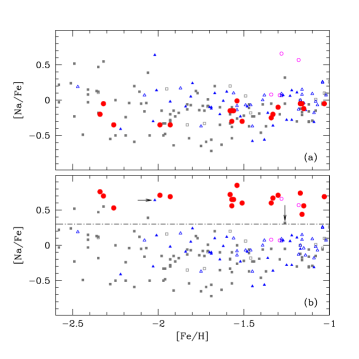
Figure 7: Comparison of [Na/Fe] values between field and GC stars as a function of metallicity. In both panels the filled red circles are for our sample of GCs, indicating [Na/Fe]_min in panel (a) and [Na/Fe]_max in panel (b), with the dot-dashed line at [Na/Fe]=0.3 (see text). [Na/Fe] ratios for field stars are the same in both panels and are taken from Fulbright et al. (2007: magenta open circles, bulge stars), Gratton et al. (2003a: blue filled triangles for accreted and open triangles for dissipation components, respectively), and Venn et al. (2004: grey filled squares for halo and open squares for thick disk stars, respectively). Small arrows in panel (b) indicate the two field stars that seem genuine second generation stars evaporated from GCs (see text) .

Observational constraints to the ratio between primordial and second generation stars may be obtained by comparing the number of stars within the GCs with that of the related field population. To have an estimate of the amount of mass lost by GCs during their evolution, we may use the peculiar composition of GC stars, namely the large excesses of Na that are often observed in GC stars, to trace these lost stars in the field. Fig. 7 shows the run of [Na/Fe] among field stars, comparing it to the extremes of the distributions for GC stars. To this purpose, we collected data for field stars from three different sources: Gratton et al. (2003a), Venn et al. (2004), and Fulbright et al. (2007). Beside the abundance ratios, they indicated the population of each star on the basis of the kinematics. Gratton et al. divided stars into ”accretion” and ”dissipation”, while Venn et al. used the more common separation between halo and disk (the correspondence accretion/halo and dissipation/disk is largely true for the stars in common); finally all stars from Fulbright et al. are bulge ones. In Fig. 7 we plot field stars -taken only once if they are present in more than one source- between metallicity $-2.5$ (to fit the lower limit of the GC metallicity range) and $-1$ (to avoid thin disk stars). In the upper panel we also plot [Na/Fe]_min for our GCs, i.e. the original, first generation value that sits in the middle of the field stars distribution. In the lower panel we plot instead [Na/Fe]_max for our GCs, i.e. the second generation value, well above the bulk of field stars.

Examining this plot, we find that while most of the field stars roughly have [Na/Fe]$\la 0$, there are a few objects with rather large excess of Na, comparable to that observed in second generation stars of GCs. In the sample of 144 field stars with [Fe/H]$<-1$, there are six stars with [Na/Fe]$>0.3$; for comparison, 50% (735 over 1483) of the stars in our survey of GC stars have such large Na excesses. However, only two of these field stars are likely to be second generation stars evaporated from GCs: they are HD74000 and HIP37335 (=G112-36). These two stars are also moderately depleted in Li (Hosford et al. 2009; Pilachowski et al 1993), as expected for second generation stars in GCs (see Pasquini et al. 2005). The remaining four Na-rich stars are extremely metal-poor stars residing in binary systems, and the Na excess may be attributed to mass transfer. Two of them (CS22898027 and CS22947187) are C-rich stars. G246-38 is extremely Li-poor (Boesgaard et al. 2005). Finally, also HD178443 is a giant in a binary system. While the statistics is poor, we may conclude that some 1.4% of the field metal-poor stars are likely Na-rich stars evaporated from GCs. Since these are half of the GC stars, we may conclude that stars evaporated from GCs make up 2.8% of the metal-poor component of the Milky Way. We may compare this value with the current fraction of stars in GCs, that is 1.2% using the Juric et al (2008) in situ star counts, and 5% using the Morrison (1993) ones (we neglect the impact of selective loss of small mass stars; this is not too bad an approximation because spectroscopic data are only available for stars with typically the current TO mass). We conclude that the GCs should have made up some 4% of the original mass of metal-poor stars, if Juric et al. star counts are used, and as much as 7.8% adopting the Morrison ones. Note that these values may still be underestimates. In fact, if the cooling flow scenario is correct, second generation stars were originally a very kinematically cold population; this means that they evaporated from the GCs only after dynamical relaxation led to energy equipartition, $\sim 1$ Gyr after the GC formation, i.e., much later than the formation phase. Then, there should be many more primordial stars of GCs now in the field, lost during the early phases. As discussed above, these values should be increased by an order of magnitude.

The conclusion is that precursors of GCs likely had a baryonic mass $\sim 20$ times larger than the current mass (if both the efficiency of star formation and the huge star loss factors are taken into account). If they also contained dark matter, they were likely two orders of magnitudes larger than they currently are, with total masses up to a few $10^{8}\leavevmode\nobreak\ M_{\odot}$, that is the size of dSph’s (see also Bekki et al. 2007).

We propose that the fraction of the primordial population lost by GCs is a major building block of the halo, although we do not exclude other minor contributors. This is supported by many other arguments, including their total mass, the metallicity distribution, and the location within the Milky Way; all these are discussed in a separate paper (Gratton et al. in preparation). GCs might have played a similar role in the formation of the metal-poor component of the thick disk ([Fe/H]$<-1$), while the specific frequency is much lower (by an order of magnitude) for the metal-rich component ([Fe/H]$>-1$), and they are obviously absent from the thin disk.

The formation phase of GCs may be very important to understand star formation in the early phases of the Milky Way (and likely of other galaxies). Any information on the composition of the primordial population would help to shed light on the formation mechanism of GCs. We will now examine what evidence can be obtained from our data.

4.2 The chemical evidence: the primordial abundance ratios and the scenario for GC formation

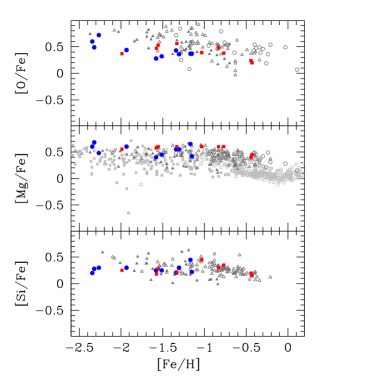
Figure 8: [O/Fe]_max, [Mg/Fe]_max, [Si/Fe]_min for our programme clusters (large filled red squares for disk/bulge clusters and blue circles for inner halo clusters, here and in the following figures) as a function of the metallicity [Fe/H], superimposed to field stars from literature (grey symbols).

4.2.1 $\alpha-$elements

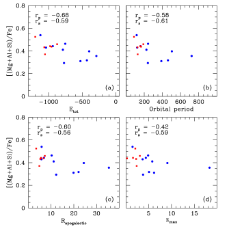
Figure 9: Relation of the ratio [(Mg+Al+Si)/Fe] as a function of several orbital parameters: (a) total energy of the orbit, (b) orbital period, (c) apogalatic distance, and (d) maximum distance above the galactic plane. Also indicated are the Spearman and Pearson correlation coefficients.

As demonstrated by several authors (Gratton et al. 1996, 2000, 2003a,b; Fuhrmann 1998, 2004), the [$\alpha$/Fe] ratio is a good population discriminator. Nissen & Schuster (1997) found that halo subdwarfs have an [$\alpha$/Fe] ratio on average lower and with more scatter than that typical of the thick disk population at the same metallicity, a result later confirmed by several other investigations (see e.g. Gratton et al. 2003b).

While several of the $\alpha$-elements are involved in the nuclear cycles related to high temperature H-burning, there are many possible indicators of the primordial [$\alpha$/Fe] ratio that we can obtain from our data. A short list includes the maximum O and Mg abundances ([O/Fe]_max and [Mg/Fe]_max), the minimum Si abundance ([Si/Fe]_min), the total Mg+Al+Si content [(Mg+Al+Si)/Fe] (see Sect. 3.4 and footnote there), and the average of [Mg/Fe]_max, [Si/Fe]_min, and the typical $\alpha-$element Ca. All these indicators give concordant results. In the following, we will mainly use the total [(Mg+Al+Si)/Fe] content.

In Fig. 8 we plotted the run of the original abundance ratio of various $\alpha-$elements with [Fe/H]: [O/Fe]_max, [Mg/Fe]_max, and [Si/Fe]_min. In the same Figure, we also plotted the distribution of field stars from Fulbright (2000), Gratton et al. (2003a), Reddy et al. (2006), Venn et al. (2004), Fulbright et al. (2003,2006). GCs lie close to the location of the field stars, specially considering possible offsets among different analyses.

We do not have an a priori idea of what we should expect for the exact form of most of the relations between the new parameters we are introducing and global cluster parameters, hence we will adopt the simpler one, a linear relation. These relations are evaluated using the Pearson coefficient for linear regressions and the Spearman coefficient of rank correlation, that can be used to characterise the strength and direction of a relationship of two given random variables (e.g. Press et al. 1992).

Tight relations are obtained between the overabundance of $\alpha-$elements (represented e.g., by Mg+Al+Si) and orbital parameters (confirming earlier findings by Lee and Carney 2002). In Fig. 9 we show the relations of the ratio [(Mg+Al+Si)/Fe] with total energy of the orbit, orbital period, apogalactic distance, and the maximum distance above the galactic plane. The correlation coefficients, represented by the Spearman and Pearson coefficients ($r_{s}$ and $r_{p}$), are high; they would further increase excluding NGC 5904 (M 5), the cluster affected by the largest uncertainties in the orbit.

Similar trends are seen when plotting the overabundance of Ca or the average between Ca and Ti i. It seems that clusters populating large-sized, more eccentric orbits, with large apogalacticon distances (i.e., mostly the inner halo GCs, in our classification), also have a proclivity to have a lower abundance of elements produced in $\alpha-$capture processes. We consider these results as an indication that the initial position affected the chemical enrichment of GCs

Is there a risk of a bias introducing spurious trends among orbital and chemical parameters? We believe that the correlation existing in our sample between absolute magnitude $M_{V}$ and distance (Sect. 3.3) is not a source of concern. We found that the total Mg+Al+Si sum is anticorrelated (with moderate significance, between 90 and 95%) with $M_{V}$: the [(Mg+Al+Si)/Fe] ratio is lower in more massive clusters. However, we found that there is a slight trend for orbital parameters to be $correlated$ with the cluster mass (luminosity) for our distance limited sample. Albeit scarcely significant from a statistical point of view, this trend is present also in the control sample of GCs with $D_{sun}<12.9$ kpc and known orbital parameters. Thus, when taken together, these opposite trends should combine in such a way to erase any dependence of the total Mg+Al+Si sum on orbital parameters, whereas we find good and significant relations. We conclude that these trends are likely significant, and should be considered when discussing scenarios for cluster formation.

We conclude that disk and halo GCs share the same [$\alpha$/Fe] ratio of thick disk and halo stars respectively. As observed in the field, halo GCs have on average smaller excess of $\alpha-$elements, and a scatter larger than that observed for the (thick) disk populations. From the [$\alpha$/Fe] ratios collected in the Appendix we found that below a metallicity of [Fe/H]$=-1$, the average values are $+0.42\pm 0.01$ dex ($rms=0.05$ dex from 15 GCs) for disk/bulge clusters and $+0.36\pm 0.02$ dex ($rms=0.07$ dex from 14 GCs) for inner halo ones.

The explanation that we propose here is not the classical one requiring the contribution of SNe Ia to raise the iron content, hence lower the [$\alpha$/Fe] ratio. We propose the possibility that the contribution of core-collapse SNe to metal enrichment is weighted towards higher-mass SNe for the precursors of lower-mass clusters: the most kinematically energetic products (rich in particular in $\alpha-$elements) might have been lost in more massive GCs, due to a powerful wind. Evidence for such a wind is found around very massive and young star clusters, like that observed in NGC 6946 (Sanchez Gil et al. 2009). Note also that in the Milky Way these massive GCs are preferentially found in the inner halo. This explanation is substantiated by the comparison of M 5 and M 4, providing a solution to the conundrum described in Sect. 3.3 .

4.2.2 Aluminium

In Paper VIII we presented the run of [Al/Fe]_min with [Fe/H] in GCs. [Al/Fe]_min is expected to represent the Al abundance of the primordial population. We underlined there the large scatter observed in this diagram, which exceeds the observational uncertainties by far; we also noticed that there is a group of clusters, mainly belonging to the inner halo, characterised by very low values of [Al/Fe]_min. Similar results were obtained previously for individual clusters (see e.g. Melendez & Cohen 2009), but our extensive survey shows that this is a widespread property of GCs.

However, Fe is not the best reference element for Al, because it has a very different nucleosynthesis. Cleaner insight can be obtained considering Mg as reference. Mg and Al may both be produced by massive stars exploding as core collapse SNe. While Mg is an $\alpha-$rich element, whose production is primary, Al requires the existence of free neutrons for its synthesis, and therefore its production is sensitive to the initial metallicity (Arnett & Truran 1969; Truran & Arnett 1971; Woosley & Weaver 1995). The exact dependence of the ratio of Al to Mg as a function of overall metallicity has never been defined satisfactorily by theory, but it should likely show some sort of secondary behaviour with respect to Mg.

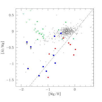
Figure 10: Run of the [Al/Mg] ratio as a function of the [Mg/H] ratio in field stars (grey-tone open circles), globular cluster in our sample (red and blue filled circles and squares, respectively) and stars in dSphs (green triangles, the open ones are upper limits in Al, see text for references). The [Al/Mg] ratio in our sample refers to primordial abundances, namely [Al/Fe]_min and [Mg/Fe]_max. The dot-dashed line indicate the line of secondary production [Al/Mg]=[Mg/H].

Fig. 10 shows the run of [Al_min/Mg_max] (that is the ratio for the primordial population) with [Mg_max/H] for our programme cluster. We also plot, with different symbols, the run of [Al/Mg] with [Mg/H] for metal-poor field stars in the Milky Way (Fulbright et al. 2007; Reddy et al. 2003; Gehren et al. 2006; Jonsell et al. 2005; Fulbright 2000), as well as for stars in dSph galaxies (Koch et al. 2008; Geisler et al. 2004; Shetrone et al. 2001, 2003; Sbordone et al. 2004). As shown by Gehren et al. (2006), the local subdwarfs have markedly different [Al/Mg], depending on their kinematics: halo subdwarfs have much lower [Al/Mg] than thick disk ones, so much that Gehren et al. proposed to use this ratio as a population diagnostics. The locus occupied by primordial populations in most GCs is clearly distinct from that for the thick disk subdwarfs, and close to that defined by halo subdwarfs. Several clusters, including the most massive ones, have very low primordial Al abundances and lie close to the line of secondary production: [Al/Mg]=[Mg/H]. The exception consists in a few small clusters (NGC 288, NGC 6121, NGC 6171, NGC 6838), that have large primordial Al abundances. A multivariate analysis, using [Mg_max/H] and $M_{V}$ as independent variables, and [Al_min/Mg_max] as dependent one, yields:

$$[{\rm Al_{\rm min}}/{\rm Mg_{\rm max}}] =(-0.01\pm 0.24)+(0.66\pm 0.14)[{\rm Mg_{\rm max}/H}]+$$ (1)

$$(0.13\pm 0.06)({\rm M_{V}}+7.5),$$

with a highly significant linear correlation coefficient of r=0.80 (16 clusters, 13 degrees of freedom). This behaviour is different from what is observed in dSph’s, that are typically characterised by rather large Al abundances.

4.2.3 A scenario for the formation of GCs

How may we explain this behaviour? First, the primary-like run of Mg and Al observed in disk subdwarfs requires that most of the Al in these stars was produced in a site different from massive stars (where the production is secondary). Second, we observed very high Al_max abundances within second generation stars in GCs (Paper VIII, and Table LABEL:t:tabnoi) even exceeding the values observed in disk subdwarfs, and similar to those observed in dSph’s stars. This suggests an obvious astrophysical site where these large amounts of Al can be produced: the same stars responsible for the Mg-Al anticorrelation (either fast rotating massive stars - FRMS - or intermediate mass AGB stars). In this case the very low Al abundances, characteristic of the primordial population of massive GCs, may be explained if the raise in metal content in the environment where these stars formed was so fast that no star with intermediate metallicity could form. On the other hand, pre-enrichment should have had to be more gradual for small mass clusters, with different generations having little difference in the Mg content, and an efficient re-processing of Mg into Al in the next generation. A similar conclusion was drawn for the case of M 71 (NGC 6838) by Melendez & Cohen (2009). However, we find that this is a general feature of GCs, even of clusters reputed younger with respect to the disk ones. This is unlikely to be a coincidence, rather is more probably related to the typical sequence of events that led to cluster formation.

This consideration suggests a (still qualitative) sketch for the formation of typical massive GCs, which is a more elaborated and updated version of what proposed more than thirty years ago by Searle & Zinn (1978) and later elaborated by many other authors (see e.g. Böker 2008 and references therein).

1. Consider a cosmological fragment/satellite of $10^{6}-10^{9}\leavevmode\nobreak\ M_{\odot}$  i.e. the same range of masses of dSph’s, but which is near the Milky Way (R${}_{GC}\sim 10$ kpc) at a very early epoch ($<2$ Gyr from Big Bang). In a cold dark matter (CDM) scenario, we expect many such satellites to have existed (see e.g. Bromm & Clarke 2002; De Lucia & Helmi 2008). At this very early epoch, this satellite is still made of dark matter and gas ($10^{5}-10^{8}\leavevmode\nobreak\ M_{\odot}$), with negligible/small stellar contribution and metal pre-enrichment, depending on its age, i.e., on the time allowed for an isolated evolution before the phases described in the following.

2. Likely due to its motion, which brings the cluster in proximity of the denser central region of the Milky Way, this fragment has a strong interaction, possibly with the same early disk of the Milky Way or with another substructure (Bekki 2004). This strong interaction triggers an early star formation (Whitmore & Schweizer 1995). In a short timescale (a few million years) $10^{4}-10^{5}\leavevmode\nobreak\ M_{\odot}$ of gas are transformed into stars; the most massive of these stars explode as SNe after $\sim 10^{7}$ yr. Hereinafter, we will call this population $precursor$, because while needed to form the GC itself, it is unlikely that we will find any representative of this population within the present GC (see below).

3. The precursor core collapse SNe have two relevant effects: i) they enrich the remaining part of the fragment/satellite of metals, raising its metallicity to the value currently observed in the GC; and ii) efficiently trigger star formation in the remaining part of the cloud, before the intermediate mass stars can efficiently contribute to nucleosynthesis. This second episode (or phase, since it is not clear that there should not be a continuum in star formation) forms a few $10^{5}-10^{6}\leavevmode\nobreak\ M_{\odot}$ of stars, in a large association. These associations have mass and size ($\sim$ 100 pc) comparable to the knots commonly observed in luminous and ultra-luminous infrared galaxies (see e.g. Rodriguez Zaurin et al. 2007).

4. The strong wind from massive stars and core collapse SNe of this huge association disperses the remaining primordial gas on a timescale of $\sim 10^{7}$ yr (see the case of the super star cluster in NGC 6946, Sanchez Gil et al. 2009).

5. While the large association is expanding, the low velocity winds from FRMS or, perhaps more likely, from the more massive intermediate mass stars feed a cooling flow, that forms a kinematically cool population at the centre of the association (D’Ercole et al. 2008). Possible examples of objects in this phase are Sandage-96 in NGC 2403 (Vinko et al. 2009) or the super star cluster in NGC 6946 (Hodge 1967, Larsen & Richtler 1999, Larsen et al. 2006). A fraction of the primordial population stars (but very few precursors if any, since they are much rarer and possibly were at some distance from the newly forming cluster) remains trapped into the very compact central cluster formed by this second generation stars. This is the GC that may survive over a Hubble time, depending on its long-scale dynamical evolution, and that we observe at present.

6. Core collapse SNe from this second generation sweep the remaining gas within the cluster, terminating this last episode of star formation. This occurs earlier in more massive clusters: these clusters will be then enriched by stars over a restricted range of mass (only the most massive among the potential polluters), leading to very large He abundances. Hence, there should be correlations between He enrichment, cluster mass, and fraction of primordial stars. Note however that this may occur naturally only in a cooling flow scenario, where second generation star formation is well separated from the evolution of individual stars. In the original FRMS scenario of Decressin et al. (2008), second generation stars form within the individual equatorial disks around the stars, as a consequence of the large mass loss rate and fast rotation. Within this scenario, it is difficult (although not strictly impossible) to link properties of individual stars to global cluster properties.

7. At some point during these processes or just after, the DM halo is stripped from the GC and merges with the general DM halo (see e.g. Saitoh et al. 2006; Maschenko & Sills 2005). It is not unlikely that the loss of the DM halo is due to the same interaction causing the formation of the GC. The cluster has now acquired the typical dynamical characteristics that we observe at present, and has hereinafter essentially a passive evolution (see e.g. Ashman & Zepf 1992).

Small and/or metal rich clusters (mainly residing in the disk) differ in many respects: forming within a disk (not necessarily the disk of the main galaxy), they have a considerable pre-enrichment of metals. In the smaller clusters, the precursor population (if it exists) does not enrich significantly the next generation, which will share the chemical composition of the field. Moreover, as we recall in Sect. 3.3, the typical luminosity of disk GCs is smaller than that of halo GCs. A large fraction of disk stars form in small clusters and association, which are easily disrupted due to infant mortality and dynamical evolution (this might be closely related to the low specific frequency of clusters in spirals: Harris and Racine 1979; Harris 1988). In addition, dynamical interaction with the disk or the presence of other nearby star forming regions might delay or reduce the efficiency of cooling flows in forming second generation stars. Observations of many clusters with multiple turn-off’s in the Magellanic Clouds (Mackey et al. 2008; Milone et al. 2009a) might indicate that this effect is not so important; see however Bastian & De Mink (2009) for a different interpretation of these observations. Finally, disk GCs all formed very early in the galactic history (Fall & Rees 1988; Zinn 1988). After these very early phases, conditions within the Milky Way disk were never again suitable for formation of very massive GCs, likely due to the low pressure characteristic of quiet disks (Ashman & Zepf 2001).

As noticed by Zinn (1985), within this scheme the different chemical history of disk and halo GCs may easily explain the most obvious characteristics of GCs, systematically observed in virtually all GC systems, such as: i) the bimodal colour and metallicity distribution , because blue clusters are essentially self-enriched, while red clusters form from pre-enriched material in the early phases of dissipational collapses (note however that there should be a few blue and metal-poor disk clusters); ii) the absence of discernible metallicity trends with R_GC for halo GCs (see Searle & Zinn 1978); and iii) the presence of relatively young GCs in the halo (Zinn 1985).

This scenario also unifies the view of GCs and dSph’s. In fact, according to this scheme, both GCs and dSph’s start as DM-dominated cosmological structures with masses in the range $10^{6}-10^{9}\leavevmode\nobreak\ M_{\odot}$. The main difference is their location with respect to the Galaxy. GCs formed from DM halos closer to the centre of the Galaxy or to other structures (even NGC 2419, the farthest known GC). They had only a limited significant independent chemical evolution prior to their interaction with the Galaxy, which occurred quite early, when the structures were still gas-rich. The age-metallicity relation for halo GCs (see Fig. 5) suggests that pre-clusters clouds that had more time to evolve, actually produced part of their metals during this pre-cluster phase. When they interacted with other structures or with the main Galaxy body itself, their independent evolution was interrupted by the sequence of phases we described above (see Melendez & Cohen 2009 for a similar view).

On the other hand, dSph’s formed much farther, at typical distances of several hundred kpc. They could have a long independent evolution before interaction (if any) with the Milky Way. Their evolution is essentially determined by their initial mass, so that they obey mass-luminosity and mass-metallicity relations. If any interaction with the Milky Way occurred (as is the case for Sagittarius), this happened once the dSph had become gas poor; this did not lead to any further GC formation (although more massive dSph’s could include a few already formed GCs).

As noticed by the referee, the scenario we considered implies that significant GC formation may still occur in gas-rich environments insofar the high pressure needed is available, e.g. due to galaxy-to-galaxy interaction. This is possibly the case of the Antennae (Whitmore & Schweizer 1995) or even of the Magellanic Clouds, where there is evidence of formation of six young clusters in the Magellanic Bridge (Irwin et al. 1985).

5 The second phase of cluster self-enrichment

In our scenario, the early phases of the evolution of the structures that will ultimately form GCs are linked to the composition of the primordial population; the late phases determine the cluster self-enrichment processes. We expect that such processes are linked to some global characteristic of GCs. In Paper VII and VIII we showed that very important rôles are played by mass and metallicity of the cluster. In this Section, we revisit this issue, considering many other parameters; a more global approach will be applied in next Section.

5.1 The chemistry of second generation stars

The chemical properties of second generation stars in GCs were discussed quite extensively in Papers VII and VIII. They may be described by the fraction of the intermediate I and of the extreme E components, and by the extreme values associated to the polluted stars using a dilution model, namely [O/Fe]_min, [Na/Fe]_max, [Mg/Fe]_min, [Al/Fe]_max. In Paper VIII we demonstrated that the ratio [Si/Fe]_max is an additional marker of second generation stars, because of the leakage of the Mg-Al cycle which produces ²⁸Si at temperatures in excess of about 65 million K (Carretta et al. 2009b; Arnould et al. 1999; Yong et al. 2005).

Table 4: Pearson’s correlation coefficients and level of significance for relations in P, I, and E stars

Par	IQR	P	I	E
IQR[O/Na]		+0.25 $<$90%	$-$0.49 95-98%	+0.65 $>$99%
P	+0.25, $<$90%		$-$0.91, $>$99%	+0.56, $>$99%
I	$-$0.49, 95-98%	$-$0.91, $>$99%		$-$0.85, $>$99%
E	+0.65, $>$99%	+0.56, 98-99%	$-$0.85, $>$99%
$[$(Mg+Al+Si)/Fe$]$	$-$0.56, $>$99%	$-$0.59, 99%	+0.69, $>$99%	$-$0.73, $>$99%
$[$Ca/Fe$]$	+0.03, $<$90%	$-$0.43, 90-95%	+0.52,  98%	$-$0.51, 95-98%
$[$O/Fe$]_{\rm min}$	$-$0.79, $>$99%	$-$0.37, $<$90%	+0.62, $>$99%	$-$0.78, $>$99%
$[$O/Fe$]_{\rm max}$	$-$0.23, $<$90%	$-$0.12, $<$90%	+0.40, 90-95%	$-$0.67, $>$99%
$[$Na/Fe$]_{\rm min}$	$-$0.03, $<$90%	+0.13, $<$90%	$-$0.20, $<$90%	+0.27, $<$90%
$[$Na/Fe$]_{\rm max}$	$-$0.26, $<$90%	$-$0.26, $<$90%	+0.21, $<$90%	$-$0.10, $<$90%
$[$Al/Fe$]_{\rm min}$	$-$0.46, 95%	$-$0.26, $<$90%	+0.36, $<$90%	$-$0.35, $<$90%
$[$Al/Fe$]_{\rm max}$	+0.10, $<$90%	+0.49, 95-98%	$-$0.38, , $<$90%	+0.10, $<$90%
$[$Mg/Fe$]_{\rm max}$	$-$0.42,   95%	$-$0.55, 98-99%	+0.74, $>$99%	$-$0.80, $>$99%
$[$Mg/Fe$]_{\rm min}$	$-$0.48, 95-98%	$-$0.61, $>$99%	+0.67, $>$99%	$-$0.56, 98-99%
$[$Si/Fe$]_{\rm max}$	$-$0.47, 95-98%	$-$0.21, $<$90%	+0.32, $<$90%	$-$0.38,  90%
$[$Si/Fe$]_{\rm min}$	$-$0.44, 95%	$-$0.32, $<$90%	+0.40, 90-95%	$-$0.40, 90-95%
${\rm[Fe/H]}$	+0.18, $<$90%	+0.01, $<$90%	$-$0.28, $<$90%	+0.58, 98-99%
MV	$-$0.46,95-98%	$-$0.39,   95%	+0.55, 98-99%	$-$0.61, $>$99%
age	$-$0.33, $<$90%	$-$0.40,   95%	+0.59, $>$99%	$-$0.71, $>$99%
T${}_{\rm eff}^{\rm max}$(HB)	+0.69, $>$99%	+0.45,   95%	$-$0.47, 95-98%	+0.36, $<$90%

• Note - The number of degrees of freedom is generally 17, except for the cases involving [(Mg+Al+Si)/Fe], [Al/Fe]_min, and [Al/Fe]_max, where it is 16.

In Tab. LABEL:t:corrtab we list the Pearson’s correlation coefficients, the number of degrees of freedom, and the statistical significance level of the correlations involving the extremes of the abundance distributions and the fraction of P, I, and E stars. In addition, we also considered the interquartile of the Na-O distribution IQR[O/Na]. We find several correlations with high statistical significance level (better than 99%), as can be seen from the Table. The most interesting correlations are shown in Figs. 11 to 16.

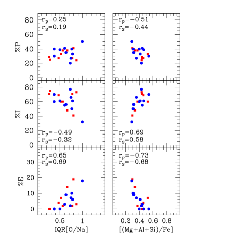
Figure 11: Left: Fraction of stars in the primordial P (upper panel), intermediate I (middle panel) and Extreme E (lower panel, with different scale on the y-axis) components of GCs as a function of the IQR[O/Na]. Right: the same, as a function of [(Mg+Al+Si)/Fe]. The Pearson and the Spearman Rank Correlation coefficients are shown in the box, here and in the next figures.

From Tab. LABEL:t:corrtab and the left panels in Fig. 11 we see that there is a tight correlation between the E fraction and the extension of the Na-O anticorrelation, IQR[O/Na]. This does not come as a surprise, since IQR[O/Na] is driven by the stars with extreme chemical modifications. The I fraction, which is the dominant group in all GCs, is anticorrelated with IQR[O/Na], while the primordial P component is not related to the extension of the Na-O anticorrelation.

The run of the P, I and E fractions as a function of the total Mg+Al+Si sum is illustrated in the left panels of Fig. 11. The fraction of stars in the P population is higher when this total sum is lower. Even tighter relations do exist for the I and E components. The sign of these relations is opposite to those with IQR[O/Na]. The combination of the left and right panels in Fig. 11 results in the statistically significant anticorrelation between IQR[O/Na] and total Mg+Al+Si sum shown in Fig. 12: clusters where the Na-O anticorrelation is more extended have a lower value of the total Mg+Al+Si sum. This result is confirmed by the relations existing between the P, I, and E fractions and [Ca/Fe] (right panels in Fig. 13). However, we also notice that these findings are strongly influenced by the two bulge clusters NGC 6388 and NGC 6441.

The E population is the only one showing a significant correlation with [Fe/H]. However, this is not surprising, because we found (Carretta et al. 2009a) that O_min, whose value is related to the presence of the E component, is well represented by a linear combination of M_V and [Fe/H]. We interpreted this result as a proof that the mass of the average polluters varies regularly as a function both of cluster mass and metal abundance.

In Fig. 14 (right panels) the fractions of first and second generation stars are shown as a function of the relative GC ages. These relations are statistically significant, the P and E components being anticorrelated and the I fraction correlated with age. This result might be an artefact due to the relations with $M_{V}$ (left panels of the same figure). As seen in Sect. 3, the more massive clusters in our sample are those in the inner halo, where the younger clusters reside. However, we cannot exclude other factors. For instance, the presence of a population with enhanced He might alter the derivation of ages; this is discussed in detail in Gratton et al. (2010).

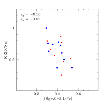
Figure 12: Extension of the Na-O anticorrelation, measured by the IQR[O/Na], as a function of the total sum of Mg+Al+Si atoms for our sample of clusters.

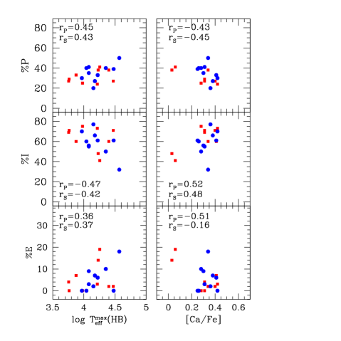
Figure 13: Left: fraction of stars of the P, I and E components (upper, middle and lower panels, respectively) as a function of log T${}_{\rm eff}^{\rm max}$(HB). Right: the same, as a function of the mean [Ca/Fe] ratio.

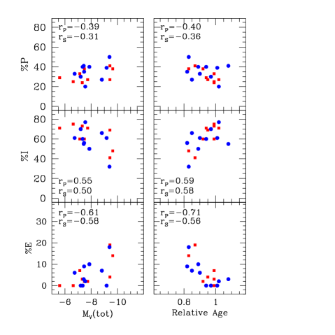
Figure 14: Left panels: The fraction of stars in the P, I and E components of second generation stars as a function of the total absolute magnitude (hence, mass) of clusters. Right: the same, as a function of relative age.

In summary:

• a P component of first generation stars is present in each GC; its incidence does not depend on the cluster metallicity, being approximatively constant (at a level of about one third of the cluster stars, Paper VII) in each GCs. This component does not affect the extension of the Na-O anticorrelation, but it is less conspicuous in GCs with higher abundances of $\alpha-$elements.

• the bulk of second generation stars is composed of stars with moderate alterations in the light elements Na, O, Mg, Al participating to proton-capture reactions in H-burning at high temperature (see Paper VII). This I component is lower in GCs with longer Na-O anticorrelations, and this fraction is higher in GCs with larger $\alpha-$element ratio.

• the E component, with extreme changes in light element abundances with respect to first generation stars, is not present in all clusters (Paper VII). It is anticorrelated to the complementary I component, and is the key component driving the extension of the Na-O anticorrelation, showing a very tight and significant correlation with IQR[O/Na]. The E component decreases with increasing overabundance of $\alpha-$elements.

In the following, we will analyse the relations between the chemistry of different sub-populations and global cluster parameters.

5.2 Extension of the Na-O anticorrelation and (blue) HB

We demonstrated in Carretta et al. (2007d) that there is a tight correlation between IQR[O/Na] (derived from part of our sample or from the literature) and the maximum temperature of HB stars, $\log{\rm T}_{\rm eff}^{\rm max}$(HB) (Recio-Blanco et al. 2006). To verify that this relation holds also for the more extended sample of clusters considered here, we complemented the values of $\log{\rm T}_{\rm eff}^{\rm max}$(HB) obtained by Recio-Blanco et al. with new ones. We employed good quality CMDs (Bellazzini et al. 2001 for NGC 288; Marino et al. 2008 for NGC 6121; Rosenberg et al. 1999 for NGC 6254; Momany et al. 2003 for NGC 6752; Vargas Alvarez & Sandquist 2007 for NGC 6809) with the same HB models (Cassisi et al. 1999) used by those authors. Furthermore, we replaced the values of IQRs of Carretta et al. (2007d) that were derived from the limited samples of stars with UVES spectra available at the time, with new ones obtained from the full sample of stars with Na and O determinations from GIRAFFE and UVES in all the 19 GCs in our sample (Tab. LABEL:t:tabnoi). We fully confirm our previous findings, as seen in Fig. 15.

The position of M 15 (NGC 7078) in Fig. 15 is somewhat uncertain. The value from literature lies very well on the relation defined by all other clusters, while the value we derive is more offset from the main trend. Since M 15 is among the most metal-poor GCs and our GIRAFFE resolution is worse than the one in Sneden et al. (1997), it is possible that we missed some very O-poor or Na-poor stars. However, the O abundance of two most O-poor stars in Sneden et al. is flagged as uncertain. With these caveats in mind, we adopt here the value of the IQR[O/Na] for M 15 derived in our analysis for homogeneity. The correlation is anyhow very tight: the Spearman test returns coefficients $r_{S}$ of 0.69 (with our value for M 15), 0.82 (with M 15 from literature), or 0.81 (without M 15). The probability to get such a tight relation by chance is negligible: the (one-tailed) $t-$test returns values of 2$\times$10^-4, 1$\times$ 10^-6, or 4$\times$ 10^-6 in the three cases, respectively.

We confirm that this is a real, very strong relation: the first conclusion we can draw is that the same mechanism drives/affects the extent of the pollution on the RGB and the morphology of the bluest end of the HB.

However, this can be only considered $a$ second parameter: the global distribution of stars on the HB [as indicated e.g., by the HB ratio HBR=(B-R)/(B+R+V) -see Harris 1996 and web updates] is $not$ correlated with IQR[O/Na], i.e. with the extension of the Na-O anticorrelation, as already discussed by Carretta (2006) and Carretta et al. (2007d). The relation between the distribution of stars along the HB and the Na-O anticorrelation is further discussed in a separate paper (Gratton et al. 2010).

Finally, the relations of the three individual stellar components P, I, E with log T${}_{\rm eff}^{\rm max}$(HB), shown in the right panels of Fig. 13, simply reflect the correlations and anticorrelations of the latter with IQR[O/Na].

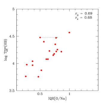
Figure 15: Interquartile range of the [O/Na] ratio as a function of the maximum temperature reached on the HB (taken from Recio-Blanco et al. 2006 or derived here). The line connects the value for M 15 based on our data and the one derived from literature (open green triangle, see text).

5.3 Extension of the Na-O anticorrelation and total cluster mass

Possibly a major result of our analysis is the good correlation we found between the IQR[O/Na] and the present-day total mass of the GCs (using the absolute magnitude M_V as a proxy for the mass), see Table LABEL:t:corrtab and Fig. 16. A large mass seems to be a requisite for an extended anticorrelation. This is not unexpected, because Recio-Blanco et al. (2006) already found a good correlation between total mass and highest temperature on the HB, and in the previous Section we found that the latter is strictly related to the extent of the Na-O anticorrelation.

The correlation found in Recio-Blanco et al. is also a good test for the reliability of our sample against a possible bias related to selection criteria. We do not have values of IQR[O/Na] for all clusters in the Harris catalogue: however, our distance-limited sample of 19 GCs shows a correlation between $M_{V}$ and log T${}_{\rm eff}^{\rm max}$(HB), with a Pearson correlation coefficient $r_{p}=-0.47$, 17 degrees of freedom, significant at better than 95% level of confidence. The same correlation is present in all clusters in the Harris catalogue with available log T${}_{\rm eff}^{\rm max}$(HB) ($r_{p}=-0.43$, 54 GCs) and for clusters in the control sample restricted to distances less than 12.9 kpc from the Sun ($r_{p}=-0.52$, 42 GCs), both significant to more than 99%.

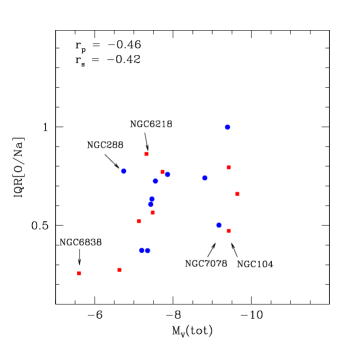
Figure 16: The extension of the Na-O anticorrelation (measured using IQR[O/Na]) as a function of the clusters’ absolute magnitude M_V from Harris (1996). The Pearson correlation coefficient is given and five GCs discussed in the text are indicated.

Thus this correlation is not due to selection bias. Moreover, since we included GCs with all morphologies of HB in our sample, it is not biased against HB type or log T${}_{\rm eff}^{\rm max}$(HB). It follows that the correlation we found between IQR[O/Na] and $M_{V}$ is real.

The explanation of this correlation is likely quite complex. On one hand, it is clear that only massive enough cluster can have a second generation. However, i) (almost) all GCs are massive enough (while open clusters likely are not, see Fig. 3), and ii) IQR[O/Na] does not depend on the fraction of second generation stars (that is on I+E, or P=1-(I+E)). Rather, IQR[O/Na] is correlated with E, and anticorrelated with I (see left panels of Fig. 11). This indicates that what is related to $M_{V}$ is the extreme of the anti-correlation, not its median value. This has been already found in Paper VII and VIII, where we showed that O_min and Al_max are strongly correlated with a combination of $M_{V}$ and [Fe/H]. In these papers we connected this fact to the typical mass of the polluters: the larger this mass, the higher the H-burning temperature, the lower is O_min and the higher is Al_max.

Hence, available data indicate that the typical polluter mass is related to $M_{V}$ (i.e., total cluster mass). To explain this relation, either the maximum or the minimum mass (or both) defining the range of polluters is changing. This might be understood quite easily in the case of AGB polluters. The maximum mass may be reduced if the cooling flow is delayed due to the presence of adjacent regions where massive stars are still present, as expected e.g. from formation of clusters in spiral arm. The minimum mass may be larger in more massive clusters: the larger the cluster mass, the faster the critical mass needed for second generation star formation is reached, before the earliest second generation SNe explode, halting further star formation. In the case of massive stars polluters, the arguments are more complex but similar: only stars formed by the ejecta of the most massive stars may contribute if the cluster mass is very large, perhaps due to devastating effect of super-winds blowing in very massive clusters.

However, the scatter we observe in Fig. 16 suggests that high mass alone is not a sufficient condition.

Clusters lying off the global relation, at the left edge, namely NGC 288, NGC 6218, (M 12) and NGC 6838 (M 71) might be reconciled with the bulk of other clusters if we assume that they lost a higher than average fraction of their original mass (we already mentioned in Sect. 4.1 arguments suggesting that a noticeable fraction of the original mass of GCs is lost after the formation phase). We searched the literature for observational evidence. De Marchi et al. (2006) argue for severe tidal stripping in NGC 6218, and they estimate that the present mass of this cluster might even be only one fifth of the original one. The flat mass function of NGC 6218 is also consistent with a large fraction of stars lost by evaporation or tidal stripping. A tidal tail is also suspected to be associated to NGC 288 (Leon et al. 2000), although other studies (Kiss et al. 2007) found no extended extra-tidal structures. The most intriguing evidence of large mass loss in these later phases is maybe the one for M 71. It comes from a totally independent line of thought. With its total absolute magnitude of $M_{V}=-5.6$ (Harris 1996), this cluster is the less massive and leftmost object in Fig. 16. Elsner et al. (2008) published a study based on $Chandra$ X-ray observations of M 71; they found that there is an excess of sources for the present cluster mass, with respect to the relation defined by 47 Tuc, M 4 and NGC 6397. Another way to state the problem is that in order to bring M 71 on the relation given by the other clusters one must assume that 50 to 70% of its original mass was lost in the past. Elsner et al. use scaled values of the mass $M_{h}$ inside the half-mass radii and a relation by Kong et al. (2006) linking $M_{h}$ to the cluster absolute visual magnitude. Using the same relation, but assuming that the scaled mass of M 71 is 1 instead of 0.3, we get a value of $M_{V}=-7.2$ which would bring this cluster perfectly on the relation between IQR[O/Na] and $M_{V}$.

On the other hand, even if accounting for less massive clusters is perhaps possible, some problems are left also at the high mass end. A large mass is not always matched by a very extended Na-O anticorrelation. NGC 104 (47 Tuc) is a notable example: this cluster simply does not show very O-poor stars and presents a short/normal Na-O anticorrelation even if it is a very massive object. Some other factors must be involved. We reconsider the case of 47 Tuc in Gratton et al. (2010)

6 The next level of the game and conclusions

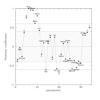
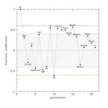
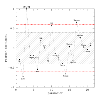
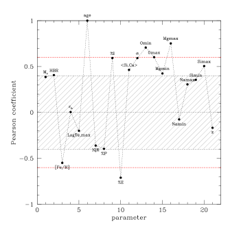
Figure 17: Example of the linear monovariate correlations found for E_tot (left upper panel), $M_{V}$ (right upper panel), [Fe/H] (left lower panel), and age (right lower panel). The first is for 15 GCs, the three other for 19 GCs. The grey zone indicates that there is no significant correlation, while the horizontal lines are drawn at (anti-)correlations larger than 0.4 and 0.6, which represent limits for a significance better than about 90% and 99% for our samples.

In the previous sections, as well as in Paper VII and VIII, we have seen the key rôle of the main parameters affecting the formation and early evolution of GCs, namely (i) the mass, (ii) the metallicity, and (iii) the galactic population/region to whom they belong (inner/outer halo vs disk). These main parameters well summarise the history of a GC, in the context of the evolution of the Galaxy itself. The correlations with chemical properties suggest that both the initial conditions at cluster’s birth and the following evolution while orbiting the Galaxy determine the resulting ratio of first and second generation stars and several other properties.

The next step is to systematically explore all the possible relations between the chemical signatures (in particular of second generation stars) of GCs and global cluster parameters, to see whether they are independent relations or may be explained with a combination of the three main parameters seen above. We can divide the parameters in five broad groups: i) structural parameters (including HBR, concentration $c$, ellipticity, $r_{h}$, $r_{t}$, and $\log$ T${}_{\rm eff}^{max}$(HB)); ii) orbital parameters and/or parameters depending on the location in the Galaxy (R_GC, $|Z|$, E_tot, age, $M_{V}$, [Fe/H]); iii) primordial abundances ([(Mg+Al+Si)/Fe] and average [$\alpha$/Fe]) and first generation ones (Mg_max, Si_min, Al_min, Na_min, O_max, plus fraction of P stars); iv) chemical parameters of second generation stars (Mg_min, Si_max, Al_max, Na_max, O_min, and fractions of I and E stars); and v) parameters linking first and second generation stars (slope of the [Al/Fe] vs [Na/Fe] ratios and IQR[O/Na]).

The GC family is a complex one, with properties depending on many parameters, often interconnected (see e.g., Djorgovski and Meylan 1994). While finding dependencies of a particular cluster property on others may be a viable approach, a more comprehensive and detailed analysis should take into account all clusters’ parameter using a multivariate approach, so we applied the Principal Component Analysis (PCA) on our set. This method has been used many times to understand the properties of the GC system (e.g., Fusi Pecci et al. 1993; Djorgovski and Meylan 1994; Recio-Blanco et al. 2006) but this is the first time that it is also extended to the properties of the different stellar generations in GCs. The method finds the correlation matrix of the whole parameter set and defines the dimensionality of the data set, i.e., the minimum number of dimensions required to fully explain the data.

Unfortunately, a rigourous study using the PCA is hampered by i) the limited sizes of the sample, 19 GCs only, since this is the only set for which detailed and homogeneous abundances of first and second generation stars are available at present; and ii) the fact that not all parameters are available for all (neither for the same) clusters. We first tried it on the maximum sample for which all the 34 above mentioned parameters are available. This means 15 GCs: NGC 6388 and NGC 6441 were excluded because they do not have orbital information, NGC 6397 because we did not measure Al, and NGC 288 because it lacks a measure of ellipticity in Harris (1996). However, excluding four clusters could result in loss of significance in some cases. For instance, $\alpha$-elements show a good correlation with $M_{V}$ in our complete sample, but not in the reduced one, possibly because two very massive clusters are excluded. We repeated the analysis using the whole GC sample, excluding those parameters that were absent for at least one of the GCs; this was possible for 21 parameters.

We give in Table 5 (available only on-line) the complete list of the correlation coefficients among the 21 parameters. We show in Fig. 17 four examples, one taken from the first computation (E_tot) and three from the second one ($M_{V}$, [Fe/H], and age); the correlation coefficients are for linear relations. Table 6 gives information on the dimensionality (the number of eigenvalues larger than 1, the limiting value usually assumed in this kind of analysis), and on the fractional and cumulative contributions of the components. This Table refers to both cases: 34 parameters for 15 GCs (first four columns) and 21 parameters for 19 GCs (last four columns). In the first case, the dimensionality is eight, the first three eigenvalues account only for 62% of the total variance, while eight components account for 93 %. In the second case, the dimensionality is five (or six), the first three eigenvalues account for 66% of the total variance, while five (six) components account for 83 (87) %.

Table 6: Eigenvalues, fractional, and cumulative contributions for the two cases discussed in the text.

34 parameters, 15 GCs						21 parameters, 19 GCs
$i$	$e_{i}$	$V_{i}$	$C_{i}$			$i$	$e_{i}$	$V_{i}$	$C_{i}$
1	11.35	33.39	33.39			1	8.25	39.30	39.30
2	5.19	15.28	48.67			2	3.61	17.18	56.48
3	4.52	13.28	61.95			3	2.11	10.05	66.53
4	2.99	8.79	70.73			4	1.86	8.83	75.36
5	2.40	7.06	77.79			5	1.56	7.51	82.87
6	2.06	6.17	83.96			6	0.96	4.57	87.44
7	1.76	5.17	89.13			7	0.69	3.20	90.74
8	1.16	3.42	92.55			8	0.61	2.91	93.65

Besides monovariate relations, we tried a semiempirical approach to explore the dependencies of cluster parameters from the fundamental quantities. In particular, we wanted to test whether the key parameters mass, metallicity, age, and orbital elements (the last two representing the position in the Galaxy) are actually those giving the most significant relations with structural and chemical parameters of GCs. We derived the correlations for parameters chosen in all the groups defined above as a function of all bi-variate combinations of $M_{V}$, [Fe/H], age, and $E_{tot}$; then, we counted the frequency of the most significant correlations (larger than 99%) for each combination in each group. The results are are given in Table 7 (on-line only) and are summarised in Table 8. The best combinations are essentially two: $M_{V}-$age and [Fe/H]-age.

Table 8: Number of significant correlations with different class of parameters.

	Struct.	Orbit./	Primord.	Chem.	Chem.	Total
		posit.	abund.	of FG	of SG
$M_{V}$	0	0	0	0	1	1
${\rm[Fe/H]}$	1	0	0	2	0	3
age	0	1	2	2	3	8
Etot	0	1	2	0	0	3
RGC	0	1	0	0	0	1
$M_{V}$,${\rm[Fe/H]}$	1	0	0	2	2	5
$M_{V}$,age	1	1	2	2	4	10
$M_{V}$,Etot	3	1	2	1	0	7
$M_{V}$,RGC	0	1	0	0	3	4
${\rm[Fe/H]}$,age	1	1	2	3	3	10
${\rm[Fe/H]}$,Etot	2	1	2	1	0	6
${\rm[Fe/H]}$,RGC	0	1	0	2	1	4
Etot,age	2	0	2	2	2	8
RGC,age	0	1	2	2	3	8
RGC,Etot	1	1	2	1	0	5

Obviously, this is meaningful only if the main parameters we are using are independent. From the monovariate correlations we see that $M_{V}$ is not correlated with age. A significant correlation does instead exist between [Fe/H] and age. This is evident both in our sample (Fig. 17) and in the global one of galactic GCs (Fig. 5), and it is stronger when individual sub-populations (inner halo vs disk/bulge) are considered. However, the age-metallicity relation is a physical one, intrinsic to the system of GCs, and not a spurious bias affecting our sample. We may safely conclude that most of the “phenotypes” of GCs can be explained rather well by the variations of three fundamental parameters: total mass, metallicity, and age, linked by the origin and the interaction of GCs in, and with, our Galaxy.

In summary, in this paper we combine the results of our extensive survey of abundances in RGB stars in 19 GCs (Carretta et al. 2009a,b,c) with previous knowledge of globular cluster, in order to discuss scenarios for their formation. The novelty of our approach is to fully take into account the fact that GCs cannot anymore be regarded as Simple Stellar Populations. For the first time it is possible to include among the properties of GCs a quantitative estimate of the ratio and of the chemical composition of different stellar generations. Our main findings are:

• We first analyse the definition of globular clusters. The presence of the Na-O anticorrelation may be very well used to separate GCs from smaller (open) clusters. Second, we divide GCs according to their kinematics and location in the Galaxy in three populations: disk/bulge, inner halo, and outer halo. We find that the LF of bona fide GCs (that is, those which exhibit the Na-O anticorrelation) is fairly independent on their population. This suggests that it is imprinted by the formation mechanism, and only marginally affected by the following evolution.

• We then use the evidence of different generations within GCs given by their chemistry, and consider separately the composition of the primordial population and of the second generation. A large fraction of the primordial population should have been lost by the proto-globular clusters. We propose that the fraction of primordial population stars lost by GCs make up the main component of halo field stars. Arguments in favour include the total number of stars, the metallicity, kinematic and density distribution, and the chemistry.

• In addition, we argue that the extremely low Al abundances found for the primordial population of massive GCs is an indication of a very fast enrichment process before the formation of the primordial population. We then suggest a scenario for the formation of GCs including at least three main phases: a) the formation of a precursor population (likely due to the interaction with the early Galaxy or with other cosmological structures similar to those that led to the formation of dwarf spheroidals, but residing at smaller Galactocentric distances), b) which triggers a large episode of star formation (the primordial population), and c) then the formation of the current GC, mainly within a cooling flow formed by the slow winds of a fraction of this primordial population. Some stars of the primordial population remains trapped in the newly forming cluster, producing the primordial component still observed in GCs. The precursor population is very effective in raising the metal content in massive and/or metal-poor (mainly halo) clusters, while its rôle is minor in small and/or metal rich (mainly disk) ones.

• We then re-examine the second phase of metal-enrichment (from primordial to second generation): we consider monovariate, bivariate relations, and an explorative PCA. Our conclusion is that most of the “phenotypes” of globular clusters (and in particular their detailed chemical characteristics) may be ascribed to a few parameters, the most important being metallicity, mass, and age of the cluster. Location within the Galaxy (as described by the kinematics) also plays some rôle, while additional parameters are required to describe their dynamical status.

The proposed scenario for the origin of GCs offers a first framework to interpret the increasing information coming from spectroscopy and photometry of GCs, and implicitly suggests several tests that can be performed. Some are currently undertaken by our and other groups. Is it possible to reproduce the observed features of the HBs in term of the fundamental parameters mass, metallicity and age (see e.g., Gratton et al. 2010)? Is the proposed scenario (precursor-present GC hosting multiple stellar generations) valid also outside the typical mass range of GCs? We are presently exploring both the very low-mass end, with the old open cluster NGC~6791, and the high-mass end, with M~54 (NGC 6715); results will be published in the next future.

While corroborating evidence is coming from these studies, several issues are still dramatically open and/or poorly explored. A full hydrodynamical treatment of the formation and early evolution of GCs is still missing, the relation between GCs and past and present dSphs needs to be well studied, the nature and the precise yields of candidate first generation polluters has still to be definitively assessed, the rôle of binaries has to be well understood, to mention only a few open problems. Although in the past few years the road to a deeper understanding of the globular clusters has been opened, the way is still long.

Appendix A Classification of Galactic globular clusters

Since the work by Zinn (1985) a few progresses were done with respect to his criteria for the separation of the sub-populations of Galactic globular clusters. Many classification schemes rest on the appearance of the clusters’ CMD and related parameters (namely metallicity, age and HBR index). However, one of the main aim of our project is to explain the HB morphology and its relations with chemical signatures of stellar generations in GC, thus we cannot use the distribution of stars along the HB as a separation criterion. In Tab. A we list the quantities used in Sect. 3.3 to separate disk/bulge clusters from the halo ones according to the combination of their location in the Galaxy and their kinematics.

As said in Sect. 3.3, outer halo clusters were simply classified as those currently located at more than 15 kpc from the centre of the Galaxy (see Carollo et al. 2008). Clusters with R_GC below 3.5 kpc were considered as bulge GCs, even though some of them might be halo clusters on very elongated orbits presently close to the pericentres. To separate the remaining clusters in inner halo and disk GCs, we computed the differences ($dV$, column 8 in Tab. A) between the observed radial velocity (corrected to the LSR) and the one expected from the Galactic rotation curve (see Clemens 1985). In the $dV-Z$ plane (where $Z$ is the clusters’ distance from the Galactic plane, in kpc, see Col. 10 of Tab. A) we defined an ellipse with equation:

$$y=\left(\frac{|dV|}{120}\right)^{2}+\left(\frac{|z|}{4}\right)^{2}.$$

Clusters with y$<$1 were classified as disk GCs, while we considered as halo GCs the ones with y$>$1, see Fig 18. Of course, a better estimate of GC kinematic is possible when the whole orbit is available. Given the quite good correlation (see Fig. 19) between $dV$ and the rotational velocity (Col. 9 of Tab. A, where $\Theta^{\star}$=$\Theta$-220) given by Dinescu et al. (1999) and Casetti-Dinescu et al. (2007), we replaced, when available, our $dV$ values with the ones provided from those studies. Since we find that $|dV|=(0.74\pm 0.06)|\Theta^{\star}|$, the definition of $y$ was in this case:

$$y=\left(\frac{|\Theta^{\star}|}{162}\right)^{2}+\left(\frac{|z|}{4}\right)^{2}.$$

It should however be clear that $dV$ is not at all a synonymous of ($\Theta$-220), and the existing correlation has only a statistical meaning.

Column 11 in Tab. A shows our classification for the population of the Galactic globular clusters in disk/bulge (D/B), inner halo (IH), outer halo (OH) and dwarf Spheroidal’s clusters (dSph). For each cluster we report the integrated magnitude (M_V, Col. 2), the horizontal branch morphology parameter (HBR, Col. 6), and the Galactocentric distance (R_GC, Col. 7) as directly retrieved from Harris’ catalogue. The metallicity values ([Fe/H] , Col. 3) were instead replaced with the determinations by Carretta et al. (2009c). Additionally, we list in Col. 4 the [$\alpha$/Fe] ratios (the corresponding references are given in the table notes). Column 5 displays the age parameter: more in detail, we computed an average value between the two different estimates by Marin-Franch et al. (2009) and De Angeli et al. (2005), after applying a correction of 0.08 to the second ones for GCs with [Fe/H] ranging from -1.8 to -1.1 dex, as suggested by a cluster-to-cluster comparison. When neither of these estimates were available, we adopted the ones calculated by Vandenberg (2000), normalised to the Marin-Franch scale by assuming that 13.5 Gyr = 1.00. We then corrected the values so obtained for the difference between the metallicities considered in those papers and those listed in Carretta et al. (2009c), transformed into [M/H] using an average [$\alpha$/Fe] of +0.4 (see Table LABEL:t:tabnoi). This correction was made using the sensitivity of age on metallicity given by Marin-Franch et al. (2009).

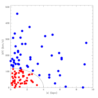
Figure 18: Classification of disk (red squares) and inner halo (blue dots) clusters. The curve is the discriminating line as obtained from our selection criteria.

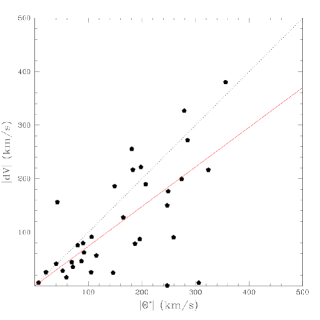
Figure 19: Absolute values of the difference $dV$ between the observed radial velocity of globular clusters and the one expected from the galactic rotation curve, as a function of the rotational velocity given by Dinescu et al. (1999) and Casetti-Dinescu et al. (2007). The dotted line indicates one-to-one correlation, while the red solid lines indicates the linear regression.

First, we decided to compare our new classification with the previous ones relying only on metallicity and HB morphology (see Sect. 3.3): as representative of this approach, we choose the work by Mackey & van den Bergh (2005). Briefly, they defined as disk component all the GCs with [Fe/H]$>$$-$0.8 dex; the so-called “old” halo and “young” halo clusters were then divided following Zinn (1993), namely by computing the offset in HB type -at a given metallicity- with respect to the fiducial line of the inner halo clusters. GCs with an offset larger and smaller than $-$0.3 in HB type were classified as old halo and young halo, respectively. The Table  9 schematically shows the comparison and emphasises the different nature of the two classifications. As (partially) expected, the matrix is not diagonal, i.e. there is not a one-to-one correlation between old halo (young halo) and inner halo (outer halo) subgroups. More in detail, the metallicity criterion is largely responsible for such a discrepancy: had we adopted the requirement of [Fe/H]$>$$-$0.8 dex, 35 of the 36 clusters that we classified as disk/bulge and Mackey & van den Bergh as old halo, should be moved into inner halo+old halo cell; while all the 5 GCs placed in the disk+young halo box should become inner halo+young halo clusters thanks to their low metallicity. However, and most important, even taking into account these changes in the relative population of the matrix cells, the resulting correspondence is not yet one-to-one: as to the inner halo GCs, 80% constitute the old halo and the remaining 20% the young halo clusters; for the outer halo GCs, the promiscuity is even larger resulting in 40% and 60%, respectively for old and young halo. This is the direct evidence of the strong difference between kinematics (and/or positional) criteria and the ones based only on metallicity and HB type.

One last word on the classification. While this work was in preparation a paper by Fraix-Burnet et al. (2009) appeared; they used a cladistic technique to divide a sample of 54 GCs into three sub-samples (called Group 1, 2, and 3 and later identify with inner halo, outer halo, and disk, respectively) on the basis of [Fe/H], M_V, T${}_{eff}^{max}(HB)$, and age. We cross-checked the assignments for the clusters in common and found a good agreement only for disk clusters, and also this in a limited sense. When they classify a cluster as disk, we agree (in 17 cases out of 18), but we have many other disk clusters that they instead classify in the halo sub-samples. In particular, for the 19 GCs in our FLAMES sample, the two classifications agree for seven clusters and disagree for seven others (five GCs are not present in their data set). We think that the main factor producing this difference is in the fact that they ignored the kinematics, although the information is present for their sample, while our method rests on that.

To conclude, we report in Table 10 the analogous of Table A but for the LMC, SMC and Fornax globular cluster system; as in the previous case, the number in brackets corresponds to the reference (for [$\alpha$/Fe], [Fe/H], age and HBR) whose decoding is given in the Notes. The integrated magnitudes $M_{V}$ for the LMC and Fornax GCs are taken from van den Bergh & Mackey (2004), while for the SMC were computed from the apparent magnitudes UBV by van den Bergh (1981) along with the distance moduli as given in those papers providing the clusters’ age. (ref. 15, 16, 17 see Table 10). As to age, for LMC and SMC GCs, since absolute values were available (see ref. given in Table 10) we report them to our relative scale adopting the previous conversion of 13.5 Gyr = 1.00. For the Fornax clusters, the ages were instead derived starting from the cluster-to-cluster relative differences ($\Delta$Age) obtained by Buonanno et al. (1998, 1999) and assuming that 1.05 = 14.2 Gyr.

[x]lccccccccccl
Name $M_{V}$ [Fe/H] [$\alpha$/Fe] $<$Age$>$ HBR R_GC dV $\Theta^{\star}$ Z Pop.
(kpc) (km/s) (km/s) (kpc)
continued.
Name $M_{V}$ [Fe/H] [$\alpha$/Fe] $<$Age$>$ HBR R_GC dV $\Theta^{\star}$ Z Pop.
(kpc) (km/s) (km/s) (kpc)
NGC 104 -9.42 -0.76  0.42(1) 0.95 -0.99   7.4  -15  59  -3.2 D/B
NGC 288 -6.74 -1.32  0.42(1) 0.90  0.99  12.0    1 247  -8.8 IH
NGC 362 -8.41 -1.30  0.30(2) 0.80 -0.87   8.9 -176 249  -6.2 IH
NGC 1261 -7.81 -1.27 — 0.79 -0.71  18.2 — — -12.9 OH
Pal 1 -2.47 -0.51 — 0.52 -1.00  17.0 — —   3.6 OH
AM1 -4.71 -1.84 — — -0.93 123.2 — — -91.3 OH
Eridanus -5.14 -1.44 — 0.71 -1.00  95.2 — — -59.6 OH
Pal 2 -8.01 -1.29 — — —  35.4 — —  -4.3 dSph
NGC 1851 -8.33 -1.18  0.38(3) 0.81 -0.36  16.7 — 87  -6.9 OH
NGC 1904 -7.86 -1.58  0.31(1) 0.89  0.89  18.8 — 137  -6.3 OH
NGC 2298 -6.30 -1.96  0.50(4) 1.01  0.93  15.7 — 246  -3.0 OH
NGC 2419 -9.58 -2.20  0.20(5) —  0.86  91.5 — —  35.9 OH
Pyxis -5.75 -1.33 — — -1.00  41.7 — —   4.8 OH
NGC 2808 -9.39 -1.18  0.33(1) 0.83 -0.49  11.1  -26 146  -1.9 IH
E3 -2.77 -0.73 — 0.92 —   7.6 — —  -1.4 D/B
Pal 3 -5.70 -1.67 — 0.83 -0.50  95.9 — 72  61.8 OH
NGC 3201 -7.46 -1.51  0.33(1) 0.82  0.08   8.9 -458 521   0.8 IH
Pal 4 -6.02 -1.46 — 0.76 -1.00 111.8 — — 103.7 OH
NGC 4147 -6.16 -1.78  0.38(6) 0.96  0.55  21.3 — 174  18.8 dSph
NGC 4372 -7.77 -2.19 — 1.00  1.00   7.1  -91 106  -1.0 D/B
Rup 106 -6.35 -1.78 -0.03(7) 0.79 -0.82  18.5 — —   4.3 OH
NGC 4590 -7.35 -2.27  0.35(1) 0.94  0.17  10.1   76 -80   6.0 IH
NGC 4833 -8.16 -1.89 — 1.01  0.97   8.7 -221 198   5.0 IH
NGC 5024 -8.70 -2.06 — 1.04  0.81  18.3 — -18  17.5 OH
NGC 5053 -6.72 -2.30 — 1.01  0.52  16.9 — —  16.1 OH
NGC 5139 -10.29 -1.64 — — —   6.4 -271 285   1.4 IH
NGC 5272 -8.93 -1.50  0.34(8) 0.88  0.08  12.2  -56 115  10.2 IH
NGC 5286 -8.61 -1.70 — 1.02  0.80   8.4  -60 —   2.0 D/B
AM 4 -1.60 -2.07 — — —  25.5 — —  16.5 OH
NGC 5466 -6.96 -2.31  0.33(9) 1.07  0.58  16.2 — 280  15.2 OH
NGC 5634 -7.69 -1.93 — — —  21.2 — —  19.1 OH
NGC 5694 -7.81 -2.02  0.16(10) 1.05  1.00  29.1 — —  17.5 OH
IC 4499 -7.33 -1.62 — —  0.11  15.7 — —  -6.6 OH
NGC 5824 -8.84 -1.94 — 1.00  0.79  25.8 — —  12.0 OH
Pal 5 -5.17 -1.41  0.17(11) — -0.40  18.6 — 178  16.7 OH
NGC 5897 -7.21 -1.90 — 1.03  0.86   7.3 -184 149  6.2 IH
NGC 5904 -8.81 -1.33  0.38(1) 0.85  0.31   6.2   26 105   5.4 IH
NGC 5927 -7.80 -0.29 — 0.91 -1.00   4.5    8  -7   0.6 D/B
NGC 5946 -7.20 -1.29 — 0.93 —   5.8 -186 —   0.8 IH
BH 176 -4.35 — — 0.55 -1.00   9.7   -3 —   1.2 Open Cluster
NGC 5986 -8.44 -1.63 — 0.97  0.97   4.8 -188 207   2.4 IH
Lynga 7 -6.37 -0.68 — — -1.00   4.2 -115 —  -0.3 D/B
Pal 14 -4.73 -1.63 — — -1.00 69.0 — —  49.6 OH
NGC 6093 -8.23 -1.75  0.24(12) 1.01  0.93   3.8 -147 247   3.3 IH
NGC 6121 -7.20 -1.98  0.51(1) 0.97 -0.06   5.9  -87 196   0.6 IH
NGC 6101 -6.91 -1.18 — 1.01  0.84  11.1 -319 —  -4.2 IH
NGC 6144 -6.75 -1.82 — 1.08  1.00   2.6 -376 356   2.3 D/B
NGC 6139 -8.36 -1.71 — 0.89  0.91   3.6 -120 —   1.2 IH
Terzan 3 -4.61 -0.755 — — —   2.4  -23 —   1.2 D/B
NGC 6171 -7.13 -1.03  0.49(1) 0.99 -0.73   3.3  -44  69   2.5 D/B
1636-283 -3.97 -1.525 — — —   2.0 — —   1.6 D/B
NGC 6205 -8.70 -1.58  0.31(8) 1.02  0.97   8.7 -199 274   5.0 IH
NGC 6229 -8.05 -1.33 — —  0.24  29.7 — —   2.7 OH
NGC 6218 -7.32 -1.43  0.41(1 ) 0.99  0.97   4.5   78  90   2.2 D/B
NGC 6235 -6.44 -1.38 — —  0.89  4.1 -105 —   2.7 IH
NGC 6254 -7.48 -1.57  0.37(1) 0.92  0.98   4.6  -36  71   1.7 D/B
NGC 6256 -6.52 -0.62 — — —   1.8  -79 —   0.5 D/B
Pal 15 -5.49 -2.10 — —  1.00  37.9 — —  18.3 OH
NGC 6266 -9.19 -1.18 — 0.89  0.32   1.7  -31 —   0.9 D/B
NGC 6273 -9.18 -1.76 — 0.99  0.96   1.6 -351 —   1.4 D/B
NGC 6284 -7.97 -1.31 — 0.91  0.88   7.6  -39 —   2.6 D/B
NGC 6287 -7.36 -2.12  0.38(13) 1.07  0.98  2.1   271 —   1.8 D/B
NGC 6293 -7.77 -2.01  0.42(13) —  0.90   1.4  -49 —   1.2 D/B
NGC 6304 -7.32 -0.37 — — -1.00   2.2   63 —   0.6 D/B
NGC 6316 -8.35 -0.36 — — -1.00   3.2 -105 —   1.1 D/B
NGC 6341 -8.20 -2.35  0.46(14) 1.11  0.91   9.6   79 187   4.7 IH
NGC 6325 -6.95 -1.37 — — —   1.1   -5 —   1.1 D/B
NGC 6333 -7.94 -1.79 — —  0.87   1.7  -99 —   1.5 D/B
NGC 6342 -6.44 -0.49  0.38(15) 0.92 -1.00   1.7   74 —   1.5 D/B
NGC 6356 -8.52 -0.35 — — -1.00   7.6  -33 —   2.7 D/B
NGC 6355 -8.08 -1.33 — — —   1.8  147 —   0.9 D/B
NGC 6352 -6.48 -0.62  0.20(16) 0.87 -1.00   3.3   21 —   0.7 D/B
IC 1257 -6.15 -1.725 — —  1.00  17.9 — —   6.5 OH
Terzan 2 -5.27 -0.29 — — -1.00   0.9 -308 —   0.3 D/B
NGC 6366 -5.77 -0.59 — 0.91 -0.97   5.0  144 —   1.0 IH
Terzan 4 -6.09 -1.62  0.50(17) —  1.00   1.3  -89 —   0.2 D/B
HP 1 -6.44 -1.57  0.34(18) —  0.75   6.1  -67 —   0.5 D/B
NGC 6362 -6.94 -1.07 — 0.94 -0.58   5.1  -81 —  -2.3 D/B
Liller 1 — 0.40 — — -7.63   1.8 -165 —   0.0 D/B
NGC 6380 -7.46 -0.40 — — —   3.2  -83 —  -0.6 D/B
Terzan 1 -4.90 -1.29 — — —   2.5 -139 —   0.1 D/B
Ton 2 -6.14 -0.525 — — —   1.4    0 —  -0.5 D/B
NGC 6388 -9.42 -0.45  0.22(1) 0.87 -0.65   3.2 -204 —  -1.2 D/B
NGC 6402 -9.12 -1.39 — —  0.65   4.1  175 —   2.4 IH
NGC 6401 -7.90 -1.01 — — —   2.7   90 —   0.7 D/B
NGC 6397 -6.63 -1.99  0.36(1) 0.99  0.98   6.0  -46  87  -0.5 D/B
Pal 6 -6.81 -1.06  0.40(19) — -1.00   2.2 -177 —   0.2 D/B
NGC 6426 -6.69 -2.36 — —  0.58  14.6  103 —   5.8 IH
Djorg 1 -6.26 -2.025 — — —   4.1  335 —  -0.5 IH
Terzan 5 -7.87 0.16  0.32(17) — -1.00   2.4  138 —   0.3 D/B
NGC 6440 -8.75 -0.20 — — -1.00   1.3  256 —   0.6 D/B
NGC 6441 -9.64 -0.44  0.21(1) 0.83 -0.76   3.9   -64 —  -1.0 D/B
Terzan 6 -7.67 -0.40 — — -1.00   1.6 -168 —  -0.4 D/B
NGC 6453 -6.88 -1.48 — — —   1.8  -13 —  -0.6 D/B
UKS-1 -6.88 -0.40  0.33(15) — -1.00   0.8 — —   0.1 D/B
NGC 6496 -7.23 -0.46 — 0.87 -1.00   4.3   43 —  -2.0 D/B
Terzan 9 -3.85 -2.07 — — —   1.6  -29 —  -0.2 D/B
Djorg 2 -6.98 -0.525 — — -1.00   1.4 — —  -0.3 D/B
NGC 6517 -8.28 -1.24 — — —   4.3  110 —   1.3 D/B
Terzan 10 -6.31 -0.725 — — -1.00   2.4 — —  -0.2 D/B
NGC 6522 -7.67 -1.45 — —  0.71   0.6   38 —  -0.5 D/B
NGC 6535 -4.75 -1.79 — 0.86  1.00   3.9  310 —   1.2 IH
NGC 6528 -6.56 0.07  0.24(20) — -1.00   0.6 -146 —  -0.6 D/B
NGC 6539 -8.30 -0.53  0.43(15) — -1.00   3.1   170 —   1.0 D/B
NGC 6540 -5.38 -1.225 — — —   4.4 16 —  -0.2 D/B
NGC 6544 -6.66 -1.47 — 0.86  1.00   5.3   27 —  -0.1 D/B
NGC 6541 -8.37 -1.82  0.43(13) 1.05  1.00   2.2   28 —  -1.4 D/B
NGC 6553 -7.77 -0.16  0.26(21) — -1.00   2.2   36 —  -0.3 D/B
NGC 6558 -6.46 -1.37  0.37(22) —  0.70   1.0  187 —  -0.8 D/B
IC 1276 -6.67 -0.65 — — —   3.7  -80 —   0.5 D/B
Terzan 12 -4.14 -0.525 — — —   3.4  -67 —  -0.2 D/B
NGC 6569 -8.30 -0.72 — — —   2.9   25 —  -1.2 D/B
NGC 6584 -7.68 -1.50 — 0.89 -0.15   7.0 -255 181  -3.8 IH
NGC 6624 -7.49 -0.42 — 0.88 -1.00   1.2   44 —  -1.1 D/B
NGC 6626 -8.18 -1.46 — —  0.90   2.7   27  52  -0.5 D/B
NGC 6638 -7.13 -0.99 — — -0.30   2.3  103 —  -1.2 D/B
NGC 6637 -7.64 -0.59  0.31(23) 0.91 -1.00   1.9   72 —  -1.6 D/B
NGC 6642 -6.77 -1.19 — — —   1.7  227 —  -0.9 D/B
NGC 6652 -6.68 -0.76 — 0.91 -1.00   2.8  135 —  -2.0 D/B
NGC 6656 -8.50 -1.70  0.38(24) 1.06  0.91   4.9  156  42  -0.4 D/B
Pal 8 -5.52 -0.37 — — -1.00   5.6   67 —  -1.5 D/B
NGC 6681 -7.11 -1.62 — 0.97  0.96   2.1  -44 —  -1.9 D/B
NGC 6712 -7.50 -1.02 — — -0.62   3.5  214 183  -0.5 IH
NGC 6715 -10.01 -1.44  0.16(25) 0.87  0.75  19.2 — —  -6.5 dSph
NGC 6717 -5.66 -1.26 — 1.00  0.98   2.4  100 —  -1.3 D/B
NGC 6723 -7.84 -1.10  0.50(26) 1.01 -0.08   2.6   83 —  -2.6 D/B
NGC 6749 -6.70 -1.62 — —  1.00   5.0  130 —  -0.3 IH
NGC 6752 -7.73 -1.55  0.43(1) 1.02  1.00   5.2  -24  21  -1.7 D/B
NGC 6760 -7.86 -0.40 — — -1.00   4.8  100 —  -0.5 D/B
NGC 6779 -7.38 -2.00 — 1.10  0.98   9.7   91 259   1.5 IH
Terzan 7 -5.05 -0.12 -0.03(27) 0.53 -1.00  16.0 — —  -8.0 dSph
Pal 10 -5.79 -0.125 — — -1.00   6.4   58 —   0.3 D/B
Arp 2 -5.29 -1.74  0.34(28) 0.89  0.86  21.4 — — -10.2 dSph
NGC 6809 -7.55 -1.93  0.42(1) 1.02  0.87   3.9  -129 165  -2.1 D/B
Terzan 8 -5.05 -2.025  0.45(28) 0.97  1.00  19.1 — — -10.8 dSph
Pal 11 -6.86 -0.45 — — —   7.9   77 —  -3.5 IH
NGC 6838 -5.60 -0.82  0.40(1) 0.94 -1.00   6.7    40  40  -0.3 D/B
NGC 6864 -8.55 -1.29 — — -0.07  14.6  144 —  -9.0 IH
NGC 6934 -7.46 -1.56 — 0.88  0.25  12.8  328 279  -5.1 IH
NGC 6981 -7.04 -1.48 — 0.87  0.14  12.9  277 —  -9.2 IH
NGC 7006 -7.68 -1.46  0.28(29) — -0.28  38.8 — — -13.8 OH
NGC 7078 -9.17 -2.33  0.40(1) 1.01  0.67  10.4   63  92  -4.7 IH
NGC 7089 -9.02 -1.66  0.41(30) 0.96  0.96  10.4    5 306  -6.7 IH
NGC 7099 -7.43 -2.33  0.37(1) 1.08  0.89   7.1  214 324  -5.9 IH
Pal 12 -4.48 -0.81 -0.01(7) 0.64 -1.00  15.9 — — -14.1 dSph
Pal 13 -3.74 -1.78 — — -0.20  26.7 — — -17.5 OH
NGC 7492 -5.77 -1.69  0.34(31) 0.93  0.81  24.9 — — -23.1 OH
Notes: (1) Carretta et al. (2009b); (2) Shetrone & Keane (2000); (3) Yong & Grundahl (2008); (4) McWilliam, Geisler & Rich (1992); (5) Shetrone et al. (2001); (6) Ivans (2009); (7) Brown, Wallerstein & Zucker (1997); (8) Sneden et al. (2004); (9) McCarthy & Nemec (1997); (10) Lee et al. (2006); (11) Smith, Sneden & Kraft (2002); (12) Cavallo et al. (2004); (13) Lee & Carney (2002); (14) Sneden et al. (2000); (15) Origlia et al. (2005); (16) Feltzing et al. (2009); (17) Origlia & Rich (2004); (18) Barbuy et al. (2006, corrrected upward by 0.20 dex); (19) Lee et al. (2004); (20) Carretta et al. (2001); (21) Cohen et al. (1999); (22) Barbuy et al. (2007, corrrected upward by 0.20 dex); (23) Lee (2007); (24) Marino et al. (2009); (25) Brown et al. (1999); (26) Fulton & Carney (1996); (27) Sbordone et al. (2007); (28) Mottini et al. (2008); (29) Kraft et al. (1998); (30) Russell (1996); (31) Cohen & Melendez (2005).

Table 9: Comparison of our classification with the one by Mackey and van den Bergh 2005

	Disk/Bulge	Old Halo	Young Halo	SGR
Disk/Bulge	34	36	5	—
Inner Halo	1	23	9	—
Outer Halo	1	11	15	—
dSph	—	—	1	6

Table 10: Globular clusters of LMC, SMC, Fornax dSph and their properties

Name	$M_{V}$	[Fe/H]	[$\alpha$/Fe]	Age	HBR
NGC 1466	-7.26	-1.76(1)	—	1.04(5)	0.41(4,6)
NGC 1754	-7.09	-1.50(1,2)	—	0.96(2,3)	0.46(3,6)
NGC 1786	-7.70	-1.76(1,2,9)	0.43(9)	1.12(2,3)	0.39(6)
NGC 1835	-8.30	-1.72(1,2)	—	0.99(2,3)	0.52(3,6)
NGC 1841	-6.82	-2.02(1)	—	0.89(8)	0.72(4,6)
NGC 1898	-7.49	-1.32(1,2,10)	0.06(10)	0.98(2,3)	-0.02(3,6)
NGC 1916	-8.24	-2.05(1,2)	—	0.93(2,3)	0.97(6)
NGC 1928	-6.06	-1.27(6)	—	0.87(13)	0.94(6)
NGC 1939	-6.85	-2.02(2,6)	—	0.94(2,3,13)	0.94(6)
NGC 2005	-7.40	-1.74(1,2,10)	0.17(10)	1.02(2,3)	0.88(6)
NGC 2019	-7.75	-1.56(1,2,10)	0.28(10)	1.20(2,3)	0.61(3,6)
NGC 2210	-7.51	-1.76(1,12,9)	0.37(9)	1.05(12)	0.61(4,6)
NGC 2257	-7.25	-1.83(1,9)	0.34(9)	1.00(5)	0.46(4,6)
Hodge 11	-7.45	-2.09(1,10)	0.38(10)	1.14(5)	0.98(4,6)
Reticulum	-5.22	-1.64(1,6)	—	0.81(13)	-0.02(4,6)
ESO121-SC03	-4.37	-0.93(12,7)	—	0.71(14)	-1.00(6)
NGC 121	-7.82	-1.46(15)	0.24(18)	0.87(15)	-0.95(6)
Lindsay 1	-5.46	-1.14(16)	—	0.58(16)	-1.00(6)
Kron 3	-6.86	-1.08(16)	—	0.51(16)	-1.00(6)
NGC 339	-5.96	-1.12(16)	—	0.47(16)	-1.00(6)
NGC 361	-6.12	-1.45(17)	—	0.63(17)	-1.00(6)
NGC 416	-7.48	-1.00(16)	—	0.47(16)	-1.00(6)
Lindsay 38	—	-1.59(16)	—	0.51(16)	-1.00(6)
Lindsay 113	-5.29	-1.38(17)	—	0.31(17)	—
Fornax 1	-5.32	-2.50(19)	0.25(19)	1.04	-0.30(6)
Fornax 2	-7.03	-2.10(19)	0.31(19)	1.01	0.50(6)
Fornax 3	-7.66	-2.40(19)	0.15(19)	1.09	0.44(6)
Fornax 4	-6.83	-1.90(20)	—	0.83	-0.42(6)
Fornax 5	-6.82	-2.20(20)	—	1.08	0.52(6)

• Notes: (1) Suntzeff et al. 1992; (2) Beasley et al. 2002; (3) Olsen et al. 1998;(4) Walker 1992b; (5) Johnson et al. 1999; (6) Mackey & Gilmore 2004a; (7) Geisler et al. 1997; (8) Saviane et al. 2002; (9) Mucciarelli et al. 2009; (10) Johnson et al. 2006; (11) van den Bergh 2006; (12) Hill et al. 2000; (13) Mackey & Gilmore 2004b; (14) Mackey et al. 2006; (15) Glatt et al. 2008a; (16) Glatt et al. 2008b; (17) Kayser et al. 2006; (18) Johnson et al. 2004; (19) Letarte et al. (2006); (20) Buonanno et al. (1999).

Table 5: Correlation coefficients for 21 parameters of the 19 GCs.

	$M_{V}$	HBR	[Fe/H]	$r_{h}$	$\log T_{eff}^{max}$	relage	IQR	%P	%I	%E	$<$SiCa$>$	[$\alpha$/Fe]	Omin	Omax	Mgmin	Mgmax	Namin	Namax	Simin	Simax	Z
	1	2	3	4	5	6	7	8	9	10	11	12	13	14	15	16	17	18	19	20	21
1	–	0.304	-0.293	0.113	-0.433	0.387	-0.463	-0.393	0.551	-0.614	0.533	0.495	0.495	0.375	0.564	0.336	-0.350	0.074	0.349	0.178	0.071
2	0.304	–	-0.731	0.131	0.454	0.407	0.198	-0.204	0.329	-0.420	0.128	0.178	0.121	0.366	0.096	0.224	-0.657	-0.181	-0.244	-0.254	-0.229
3	-0.293	-0.731	–	-0.187	-0.195	-0.549	0.182	0.003	-0.277	0.585	-0.142	-0.252	-0.387	-0.658	0.045	-0.310	0.661	0.271	0.026	-0.034	0.070
4	0.113	0.131	-0.187	–	-0.157	0.005	0.138	-0.214	0.195	-0.131	0.439	0.376	-0.078	0.197	0.193	0.127	-0.146	-0.219	0.371	0.078	0.050
5	-0.433	0.454	-0.195	-0.157	–	-0.199	0.693	0.453	-0.468	0.361	-0.347	-0.333	-0.471	-0.056	-0.681	-0.272	-0.207	-0.389	-0.530	-0.334	-0.232
6	0.387	0.407	-0.549	0.005	-0.199	–	-0.332	-0.396	0.593	-0.710	0.464	0.592	0.707	0.603	0.425	0.752	-0.075	0.306	0.356	0.505	-0.167
7	-0.463	0.198	0.182	0.138	0.693	-0.332	–	0.248	-0.486	0.654	-0.188	-0.297	-0.788	-0.228	-0.475	-0.423	-0.030	-0.262	-0.438	-0.465	-0.207
8	-0.393	-0.204	0.003	-0.214	0.453	-0.396	0.248	–	-0.914	0.561	-0.484	-0.517	-0.372	-0.118	-0.615	-0.551	0.130	-0.263	-0.321	-0.206	-0.185
9	0.551	0.329	-0.277	0.195	-0.468	0.593	-0.486	-0.914	–	-0.848	0.573	0.661	0.621	0.398	0.671	0.740	-0.204	0.211	0.404	0.320	0.187
10	-0.614	-0.420	0.585	-0.131	0.361	-0.710	0.654	0.561	-0.848	–	-0.542	-0.680	-0.779	-0.667	-0.559	-0.797	0.265	-0.097	-0.397	-0.378	-0.121
11	0.533	0.128	-0.142	0.439	-0.347	0.464	-0.188	-0.484	0.573	-0.542	–	0.957	0.218	0.368	0.503	0.630	0.012	-0.032	0.801	0.473	0.153
12	0.495	0.178	-0.252	0.376	-0.333	0.592	-0.297	-0.517	0.661	-0.680	0.957	–	0.345	0.419	0.485	0.805	0.054	0.053	0.784	0.547	0.060
13	0.495	0.121	-0.387	-0.078	-0.471	0.707	-0.788	-0.372	0.621	-0.779	0.218	0.345	–	0.486	0.462	0.598	-0.074	0.372	0.336	0.561	0.074
14	0.375	0.366	-0.658	0.197	-0.056	0.603	-0.228	-0.118	0.398	-0.667	0.368	0.419	0.486	–	0.219	0.477	-0.376	-0.352	0.089	0.157	0.292
15	0.564	0.096	0.045	0.193	-0.681	0.425	-0.475	-0.615	0.671	-0.559	0.503	0.485	0.462	0.219	–	0.486	0.036	0.350	0.386	0.224	0.156
16	0.336	0.224	-0.310	0.127	-0.272	0.752	-0.423	-0.551	0.740	-0.797	0.630	0.805	0.598	0.477	0.486	–	0.108	0.277	0.476	0.599	-0.007
17	-0.350	-0.657	0.661	-0.146	-0.207	-0.075	-0.030	0.130	-0.204	0.265	0.012	0.054	-0.074	-0.379	0.036	0.108	–	0.539	0.310	0.308	-0.349
18	0.074	-0.181	0.271	-0.219	-0.389	0.306	-0.262	-0.263	0.211	-0.097	-0.032	0.053	0.372	-0.352	0.350	0.277	0.539	–	0.176	0.330	-0.536
19	0.349	-0.244	0.026	0.371	-0.530	0.356	-0.438	-0.321	0.404	-0.397	0.801	0.784	0.336	0.089	0.386	0.476	0.310	0.176	–	0.721	0.061
20	0.178	-0.254	-0.034	0.078	-0.334	0.505	-0.465	-0.206	0.320	-0.378	0.473	0.547	0.561	0.157	0.224	0.599	0.308	0.330	0.721	–	0.120
21	0.071	-0.229	0.070	0.050	-0.232	-0.167	-0.207	-0.185	0.187	-0.121	0.153	0.060	0.074	0.292	0.156	-0.007	-0.349	-0.536	0.061	0.120	–

Table 7: Correlations, with number of clusters, degrees of liberty, Pearson coefficients (without sign), and significance in percent.

	$M_{V}$	[Fe/H]	age	Etot
Structural parameters
HBR	19 17 0.30 $<$90	19 17 0.73 $>99$	19 17 0.41 90-95	17 15 0.01 $<$90
c	19 17 0.35 $<$90	19 17 0.29 $<$90	19 17 0.31 $<$90	17 15 0.03 $<$90
ellipticity	18 16 0.36 $<$90	18 16 0.05 $<$90	18 16 0.44 90-95	16 14 0.61 98-99
$r_{h}$	19 17 0.11 $<$90	19 17 0.19 $<$90	19 17 0.00 $<$90	17 15 0.33 $<$90
$r_{t}$	19 17 0.33 $<$90	19 17 0.41 90-95	19 17 0.04 $<$90	17 15 0.59 98-99
logTeff	19 17 0.43 90-95	19 17 0.20 $<$90	19 17 0.20 $<$90	17 15 0.18 $<$90
Orbital and positional parameters
RGC	19 17 0.00 $<$90	19 17 0.30 $<$90	19 17 0.24 $<$90	17 15 0.59 98-99
$|Z|$	19 17 0.02 $<$90	19 17 0.40 90-95	19 17 0.07 $<$90	17 15 0.48 95.0
Etot	17 15 0.34 $<$90	17 15 0.20 $<$90	17 15 0.64 $>99$
age	19 17 0.43 90-95	19 17 0.37 $<$90		17 15 0.78 $>99$
$M)V$		19 17 0.29 $<$90	19 17 0.39 90.0	17 15 0.34 $<$90
${\rm[Fe/H]}$	19 17 0.29 $<$90		19 17 0.55 98-99	17 15 0.20 $<$90
Primordial abundances
Mg+Al+Si	18 16 0.42 90-95	18 16 0.18 $<$90	18 16 0.77 $>99$	16 14 0.68 $>99$
$\alpha$	19 17 0.49 95-98	19 17 0.25 $<$90	19 17 0.59 $>99$	17 15 0.64 $>99$
First generation abundances
Mgmax	19 17 0.34 $<$90	19 17 0.31 $<$90	19 17 0.75 $>99$	17 15 0.61 99.0
Simin	19 17 0.35 $<$90	19 17 0.03 $<$90	19 17 0.36 $<$90	17 15 0.37 $<$90
Almin	18 16 0.19 $<$90	18 16 0.23 $<$90	18 16 0.23 $<$90	16 14 0.24 $<$90
Namin	19 17 0.35 $<$90	19 17 0.66 $>99$	19 17 0.08 $<$90	17 15 0.26 $<$90
Omax	19 17 0.37 $<$90	19 17 0.66 $>99$	19 17 0.60 $>99$	17 15 0.00 $<$90
P	19 17 0.39 90.0	19 17 0.00 $<$90	19 17 0.40 90-95	17 15 0.33 $<$90
Second generation abundances
Mgmin	19 17 0.56 98-99	19 17 0.04 $<$90	19 17 0.42 90-95	17 15 0.35 $<$90
Simax	19 17 0.18 $<$90	19 17 0.03 $<$90	19 17 0.51 95-98	17 15 0.46 90-95
Almax	18 16 0.26 $<$90	18 16 0.40 90.0	18 16 0.15 $<$90	16 14 0.13 $<$90
Omin	19 17 0.50 95-98	19 17 0.39 90.0	19 17 0.71 $>99$	17 15 0.40 $<$90
Namax	19 17 0.07 $<$90	19 17 0.27 $<$90	19 17 0.31 $<$90	17 15 0.46 90-95
I	19 17 0.55 98-99	19 17 0.28 $<$90	19 17 0.59 $>99$	17 15 0.37 $<$90
E	19 17 0.61 $>99$	19 17 0.58 99.0	19 17 0.71 $>99$	17 15 0.34 $<$90
Link first-second generation
slope[Na/Al]	18 16 0.46 95.0	18 16 0.08 $<$90	18 16 0.35 $<$90	16 14 0.34 $<$90
IQR[O/Na]	19 17 0.46 95-98	19 17 0.18 $<$90	19 17 0.33 $<$90	17 15 0.18 $<$90