Realization of the farad from the dc quantum Hall effect with digitally-assisted impedance bridges

Abstract

A new traceability chain for the derivation of the farad from dc quantum Hall effect has been implemented at INRIM. Main components of the chain are two new coaxial transformer bridges: a resistance ratio bridge, and a quadrature bridge, both operating at 1541Hz. The bridges are energized and controlled with a polyphase direct-digital-synthesizer, which permits to achieve both main and auxiliary equilibria in an automated way; the bridges and do not include any variable inductive divider or variable impedance box. The relative uncertainty in the realization of the farad, at the level of 1000pF, is estimated to be 64E-9. A first verification of the realization is given by a comparison with the maintained national capacitance standard, where an agreement between measurements within their relative combined uncertainty of 420E-9 is obtained.

1 Introduction

A number of National Metrology Institutes work on measurement setups to trace the farad to the representation of the ohm given by the dc quantum Hall effect [1, 2, 3, 4, 5, 6, 7, 8, 9, 10, 11] . The traceability chains employed involve a number of experimental steps, usually requiring not less than three different coaxial ac bridges. The bridges are complex networks of passive electromagnetic devices [12]: some of such devices are fixed (transformers and single-decade inductive voltage dividers), and several are variable (resistance and capacitance boxes, multi-decadic inductive voltage dividers). Bridges are balanced by operating on the variable devices to reach equilibrium; that is, the detection of zero voltage or current on a number of nodes in their electrical networks. Variable devices, especially inductive voltage dividers, are typically manually operated; only a few models have been described [13, 14, 7, 15] which permit remote control. Consequently, a large part of existing bridges are manually operated.

In most cases, the role of variable devices in a bridge is to synthesize signals (voltages or currents) to be injected in the bridge network to bring a detector position to zero. The signals are isofrequential with the main bridge supply, and can be adjusted in their amplitude and phase relationships. The amplitude and phase of one (or more) of the signals enters the measurement model equation, and must be calibrated (main balance), but the others (auxiliary balances) don’t need a calibration.

In this view, it is straightforward to consider a substitution in the bridge network of most, or all, variable passive devices with a corresponding number of active sinewave generators, locked to the same frequency but adjustable in amplitude and phase independently of each other. Direct digital synthesis (DDS) of sinewaves [16] is a well-established technique that permit the realization of such generators; hence, in this sense, we may speak of digitally-assisted impedance bridges when DDS generators are used. Digitally-assisted bridges impedance have been considered both theoretically [17, 18] and in a number of implementations [19, 20, 21, 22, 23, 24, 25, 26, 27, 28, 29]; some commercial impedance meters are also digitally-assisted.

In this paper, we consider for the first time the feasibility of a complete ohm to farad traceability chain based on digitally-assisted bridges. We constructed a resistance ratio bridge and a quadrature bridge, to measure capacitance (at the level of 1000pF) in terms of dc quantum Hall resistance (at the level of $R_{\mathrm{K}}/2\approx$12906.4, where $R_{\mathrm{K}}$ is the Von Klitzing constant). The bridges are automated, and a single measurement can be conducted in minutes. The estimated relative uncertainty of the capacitance determination related to the traceability chain is 64E-9.

This accuracy claim hasn’t yet been verified with a comparison with other farad realization. However, by completing the chain with an older manual transformer ratio bridge [30], we performed a comparison between the new realization and the present national capacitance standard, maintained as a group value at the level of 10pF with a relative uncertainty of 400E-9. The measurement results of the comparison are compatible within the relative compound uncertainty.

2 The traceability chain

The traceability chain which has been set up, including the steps for the comparison (Sec. 6.5) with the maintained capacitance standard is shown in graphical form in Fig. 1. Its steps are here summarized and will be described in more detail in the course of the paper.

• The quantum Hall effect is employed to calibrate a resistor $R_{\mathrm{Q}}$ having the nominal value $R_{\mathrm{K}}/2\approx$ 12906.4 and a calculable frequency performance;

• $R_{\mathrm{Q}}$ is employed in a 8:1 resistance ratio bridge to calibrate two resistance standards $R_{1,2}$, with nominal value $4\times R_{\mathrm{K}}\approx$ 103.251k, at the frequency $f\approx$1541.4Hz;

• $R_{1,2}$ are employed in a quadrature bridge to calibrate the product $C_{1}\times C_{2}$ of two capacitance standards $C_{1,2}$ with nominal value of 1000pF;

• in order to perform the comparison with the maintained capacitance standard, maintained at the level of 10pF, a capacitance ratio bridge is employed to perform a scaling up to 1000pF and the measurement of $C_{1}$ and $C_{2}$;

• a small calculated frequency correction is applied to permit the comparison.

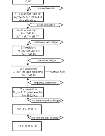
Figure 1: Graphical representation of the traceability chain for the realization of the farad unit from the quantum Hall effect.

3 Impedance standards

The standards employed in the traceability chain are:

$R_{\mathrm{Q}}$

a quadrifilar resistance standard, having a nominal value $R_{\mathrm{Q}}=R_{\mathrm{K}}/2$. Its frequency performance and reactive parameter are calculable from geometrical dimensions [31]: the result of the calculation is shown in Fig. 2. The standard is thermostated to improve its stability. The original standard has an inductance of $\approx$3H; in order to reduce its phase angle, a small gas-dielectric capacitor has been added in parallel to its current terminals.

$R_{1,2}$

two resistance standards with nominal value $R_{1,2}=4\times R_{\mathrm{K}}$. Presently, two thin film resistors encased in a metal shield and defined as two terminal-pair standards are employed. The casings are within a single air bath, having 1mK temperature stability. Two new standards with independent thermostats are under construction.

$C_{1,2}$

two gas-dielectric capacitance standards $C_{1,2}=$1nF are constructed from General Radio 1404-A standards, re-encased in a thermostated bath at 23 with 1mK stability and redefined as two terminal-pair impedance standards. Ref. [7] gives a detailed description of the construction and characterization.

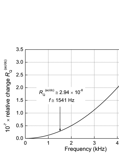
Figure 2: Frequency performance of the $R_{\mathrm{Q}}$ resistor.

4 Digitally-assisted coaxial bridges

The digitally-assisted bridges developed are a 8:1 resistance ratio bridge, and a quadrature bridge. The coaxial schematics can be seen in Fig. 3 and Fig. 4 respectively. The bridges are based on the same design concept and share common instrumentation: the polyphase generator (Sec. 4.1), the impedance standards (Sec. 3), and the detector. A photo of both bridges is shown in Fig. 5.

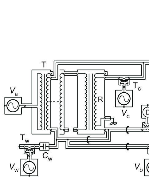
Figure 3: Simplified diagram of the 8:1 resistance ratio bridge. Black rings along the mesh are current equalizers.

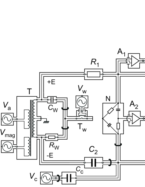
Figure 4: Simplified diagram of the two-terminal-pair quadrature bridge.

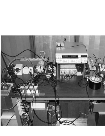
Figure 5: A photo of the two bridges. On the left the quadrature bridge; on the right the resistance ratio bridge. The instruments in the middle are common to both bridges.

4.1 Polyphase generator

Both bridges are energized (one at a time) by a polyphase DDS generator; the schematic diagram is reported in Fig. 6. The core of the generator is a commercial digital-to-analogue (DAC) board. The board is programmed for a continuous generation of sinewaves; each wave can be updated without stopping the generation (large amplitude or phase changes are gradually achieved to avoid steps in the output).

Since the sinewaves are represented by an integer number of samples (presently 628), the output frequency is finely tuned by changing the common DAC update clock frequency, typically ranging between 950kHz and 1MHz. The clock is given by a commercial synthesizer connected to the DAC board by an optical fibre link [32] to minimize high-frequency interferences. The synthesizer is in turn locked to INRIM 10MHz timebase; hence, the frequency uncertainty of the polyphase generator is better than 1E-10.

Five DAC channels are used. Four are employed on the bridge network, the fifth gives a reference signal for the lock-in amplifier which acts as zero detector. The four channels enter a purposely-built analog electronics which include, for each channel, a line receiver (which decouple the computer ground from the bridge ground), a 200kHz low pass two-pole Butterworth filter to reduce the quantization noise, and a buffer amplifier with automatic control of dc offset [33] to avoid possible magnetizations of the electromagnetic components. The analog gain of each channel can be finely trimmed.

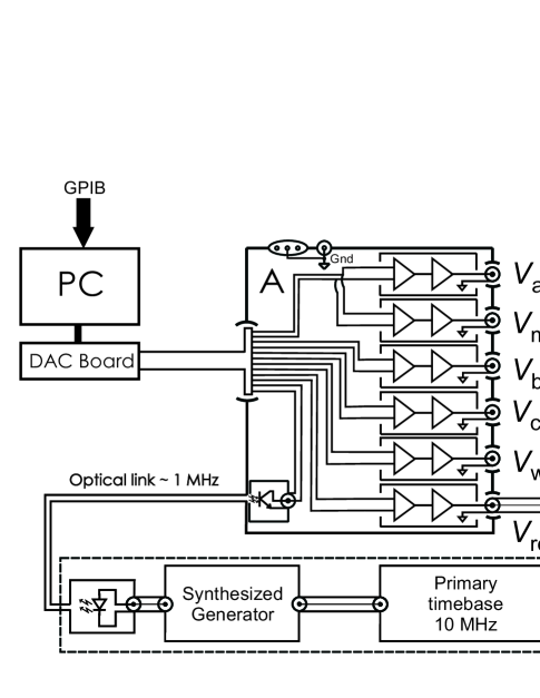
Figure 6: Schematic diagram of the sinewave synthesizer, see Sec. 4.1 for details.

4.2 Resistance ratio bridge

A simplified coaxial diagram is shown in Fig. 3. Output $V_{\mathrm{a}}$ of the polyphase generator energizes the main isolation transformer T, which has two secondary windings: one supplies the measurement current, the other energizes the magnetizing winding of the main ratio divider R. $R_{Q}$ is defined as a four terminal-pair impedance, whereas $R_{1,2}$ is defined as two terminal-pair impedance. Output $V_{\mathrm{b}}$ of the generator, with injection transformer T_b, adjusts the current in $R_{\mathrm{Q}}$. Output $V_{\mathrm{c}}$, and injection transformer T_c having ratio $D_{\mathrm{c}}$, provide the main balance by adjusting R ratio. Output $V_{\mathrm{W}}$, with transformer T_W and injection capacitance $C_{\mathrm{W}}$, provides Wagner balance. The detector D is the input of the lock-in amplifier (in floating mode), manually switched between detection points.

The result of measurement $R_{1,2}/R_{\mathrm{Q}}\approx 8$ can be expressed as

$$\frac{R_{1,2}}{R_{\mathrm{Q}}}=8\left\{1+\frac{10}{8}\cdot\frac{1}{D_{\mathrm{c}}}\cdot\frac{\left|V_{\mathrm{c}}\right|}{\left|V_{\mathrm{a}}\right|}\cos\left[\arg(V_{\mathrm{c}})-\arg(V_{\mathrm{a}})\right]-\frac{81}{8}\epsilon_{\mathrm{ph}}\right\},$$ (1)

Eq. 1 takes into account also the complex deviation $\epsilon$ of the ratio $k$ of R from its nominal value $1/9$, expressed as $k=1/9+\epsilon_{\mathrm{ph}}+j\epsilon_{\mathrm{qd}}$. R is calibrated using a bootstrap technique [34] validated in an international intercomparison [35].

4.3 Quadrature bridge

The quadrature bridge is shown in Fig. 4. The bridge measure the product $C_{1}C_{2}$ in terms of $R_{1}R_{2}$; it is an evolution of a similar bridge presented in [36].

The main ratio transformer T has a magnetizing winding (driven by generator output $V_{\mathrm{mag}}$) and a primary winding (driven by output $V_{\mathrm{a}}$). The secondary winding is a center-tapped bifilar winding providing two nominally equal outputs +E and -E.

The double equilibrium of the quadrature bridge is obtained by adjustments of the quadrature voltage (provided by generator output $V_{Q}$) and of a balancing current (provided by output $V_{\mathrm{c}}$ and an injection capacitor $C_{\mathrm{c}}$).

A fixed combining network N decouples the adjustments; detector points are monitored with low-noise amplifiers $\mathrm{A_{1}}$ and $\mathrm{A_{2}}$ and the lock-in amplifier, manually switched between the two detection points .

Output $V_{\mathrm{W}}$, with transformer T_W and injection network $C_{\mathrm{W}}$-$R_{\mathrm{W}}$, provides Wagner balance.

The reading of the quadrature bridge can be expressed as (see Ref. [12], ch. 6.2.2)

$$\omega^{2}R_{1}R_{2}C_{1}C_{2}=1+\delta$$ (2)

The real part $\mathrm{Re}\left[\delta\right]$ of $\delta$, which links principal values of $R_{1},R_{2},C_{1},C_{2}$ (the imaginary part $\mathrm{Im}\left[\delta\right]$ links resistance time constants to capacitance losses) is given by the expression

$$\mathrm{Re}\left[\delta\right]=\frac{\left|V_{\mathrm{c}}\right|}{\left|V_{\mathrm{Q}}\right|}\,\omega\,C_{\mathrm{c}}\,R_{2}\sin\left[\arg(V_{\mathrm{c}})-\arg(V_{\mathrm{Q}})\right]$$ (3)

where $\left|V_{\mathrm{c}}\right|$ and $\left|V_{\mathrm{Q}}\right|$ are the amplitudes of phasors $V_{\mathrm{c}}$ and $V_{\mathrm{Q}}$, and $\arg(V_{\mathrm{c}})$, $\arg(V_{\mathrm{Q}})$ are their phases.

Eq. 3 does not take into account possible asymmetries of transformer T; however, these are compensated by exchanging the connections of the outputs of T to the bridge network, and by averaging the two values of $\mathrm{Re}\left[\delta\right]$ obtained with the two equilibria.

4.4 Bridge operation

The bridges are operated in a similar way, with the same control program. The user interface permits to set the amplitude and relative phase of each generator output; to achieve equilibrium, an automated procedure [37] is implemented, resulting an increased speed and ease of operation. Presently the detector input must be manually switched between different detection points; despite this, equilibrium is reached from an arbitrary setting in a few minutes; if the if the bridge is already near equilibrium condition the procedure is faster.

5 Maintained capacitance unit

The Italian capacitance national standard is presently maintained as the group value of several 10pF quartz-dielectric capacitors [30]. The capacitance differences are periodically monitored, and the group value is updated by drift prediction and by participating to international comparisons [38]. The scaling from 10pF to 1000pF is performed with a manual two terminal-pair coaxial ratio bridge [30] and a step-up procedure which permits to compensate for possible deviations of the transformer ratio from its nominal value.

6 Results

6.1 Measurements of $R_{\mathrm{Q}}$

The representation of the ohm at INRIM is given [39] by the dc quantum Hall effect on the $i=2$ step, $R_{\mathrm{K}}/2\approx$ 12906.4. A dc potentiometer [40] performs calibrations of resistance standards. A time series of measurements of $R_{\mathrm{Q}}$ is shown in Fig. 7: a significant, but predictable, drift of 5n  ^-1 d^-1 is estimated.

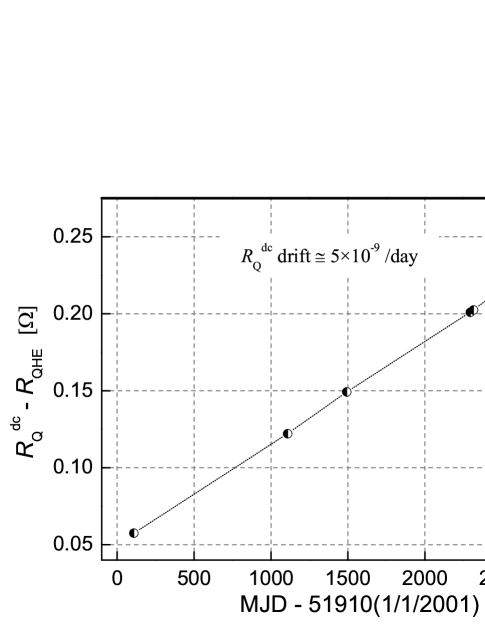
Figure 7: Time drift of the quadrifilar resistor $R_{\mathrm{Q}}$.

6.2 Characterization of the polyphase generator

As shown in Sec. 4.2 and 4.3, the reading of each bridge is given by a mathematical expression whose input quantity is the complex ratio of the nominal settings of two generators ($V_{\mathrm{c}}/V_{\mathrm{a}}$ for the ratio bridge, $V_{\mathrm{c}}/V_{\mathrm{Q}}$ for the quadrature bridge). The tracking of the different outputs of the generator (under proper loading conditions) has been adjusted and calibrated; the deviations from nominal values are within a few parts in $10^{4}$. Since the impedance standards deviate from their nominal values by less than a few parts in $10^{-5}$, and their relative phases have been adjusted, the contribution to final accuracy of each bridge caused by the generators can be kept near 1E-8.

The stability and noise of the polyphase generator can be inferred from drifts of detector readings of the bridge after an equilibrium. Fig. 8 show the time evolution of the detector reading at the combining network of the quadrature bridge, which is affected by all generator output drifts.

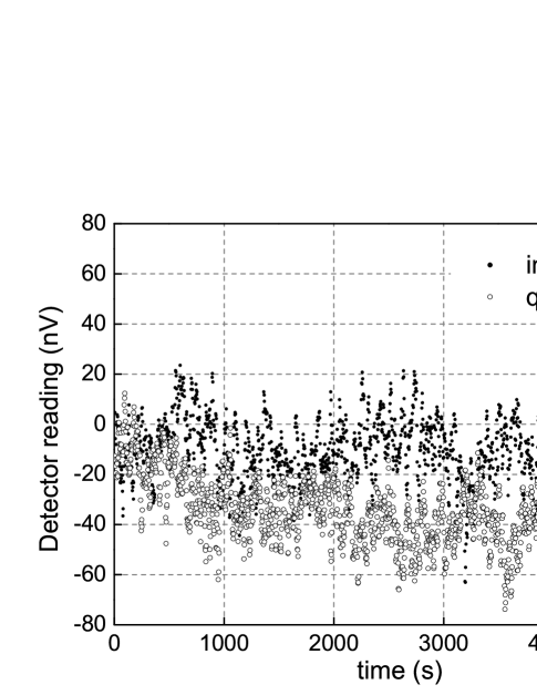
Figure 8: Typical time evolution of the detector reading (in-phase and quadrature components) at the combining network detection point of the quadrature bridge, after an equilibrium operation (for $t=0$).

6.3 Ratio bridge measurements

Fig. 9 shows the measurement of $R_{2}/R_{\mathrm{Q}}$ with the resistance ratio bridge (the result of $R_{1}/R_{\mathrm{Q}}$, not shown, is very similar) over a period of more than one year of operation. The ratio drift is caused by the compound drift of both $R_{2}$ and $R_{\mathrm{Q}}$. The inset of Fig. 9 shows the repeatability of measurements over a few days.

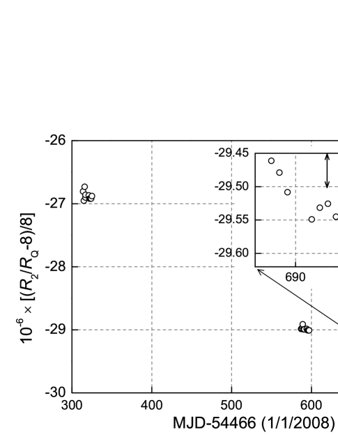
Figure 9: Results of measurement of $R_{2}/R_{\mathrm{Q}}$ with the 8:1 resistance ratio bridge over a period of 400 days. Data is expressed as relative deviation (in parts per $10^{6}$) from the nominal ratio $[R_{2}/R_{\mathrm{Q}}]_{\mathrm{nominal}}=8$.

6.4 Quadrature bridge measurements

Fig. 10 shows the measurement of $\delta$ (see Eq. 2) with the quadrature bridge over the same time period of Fig. 9. The drift is the compound drift of the standards $R_{1}$, $R_{2}$, $C_{1}$, $C_{2}$. The inset of Fig. 9 shows the repeatability of measurements over a few days.

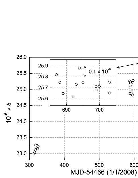
Figure 10: Results of measurement of $\delta\equiv\omega^{2}R_{1}R_{2}C_{1}C_{2}-1$ with the quadrature bridge over a period of 400 days. The inset shows the repeatability of the measurement over a few days.

6.5 Final result, and comparison with the maintained capacitance standard

Fig. 11 shows the geometric mean of $C_{1}$ and $C_{2}$ from the nominal (1000pF) value. The result is computed from all data previously described. The observed drift is attributed to coumpond drift of $C_{1}$ and $C_{2}$.

In the same figure, the result (with uncertainty bars) given by a step-up measurement from the maintained national capacitance standard is shown; a visual agreement can be appreciated. This measurement is performed at the frequency of 1592Hz and should be corrected to 1541Hz because of the frequency dependence of $C_{1}$ and $C_{2}$. Indirect measurements of such dependence, performed with the so-called S-matrix method [41] give a correction below 1E-9. An uncertainty contribution associated with the correction has been nevertheless added to the uncertainty budget (see Sec. 7).

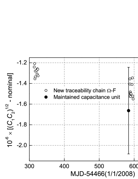
Figure 11: Comparison between quadrature bridge and step up procedure.

7 Uncertainty

Tables 1–3 give the uncertainty expression corresponding to the measurements described in Sec. 6:

• Tab. 1 lists the uncertainty contributions related to the various measurements and standards employed in the new traceability chain;

• Tab. 2 gives the uncertainty budget for the measurement of the geometric mean $(C_{\mathrm{1}}C_{\mathrm{2}})^{1/2}$ of the 1000pF capacitance standards $C_{\mathrm{1}}$ and $C_{\mathrm{2}}$ in terms of the INRIM representation of the ohm given by the quantum Hall effect in dc regime;

• Tab. 3 gives the uncertainty budget for the comparison described in Sec. 6.5 and shown in graphic form in Fig. 11.

Table 1: Measurement steps of the ohm-farad traceability chain: relative uncertainty expression (contributions and root-sum-square RSS)

Source of uncertainty	Type	$u_{\mathrm{r}}$	Note
1: Calibration of $\textit{R}_{Q}$ @ 1541Hz		nΩ⋅Ω^-1
DC calibration of $R_{\mathrm{Q}}$	A, B	25	Calibration with dc QHE
phase correction of $R_{\mathrm{Q}}$	B	12	1E-5 loss angle of 10pF capacitor
Frequency dependence	B	3	10% of calculated frequency deviation
Short-term stability	B	10	Estimated drift is $5\times 10^{-9}$/day
RSS		30
2: Resistance ratio bridge		nΩ⋅Ω^-1
Noise	A	10	Std of the mean of 10 measurements
Main balance injection	B	12	5E-4 of a 25E-6 injection
4TP impedance definition	B	10
4TP cable corrections	B	1	See [12]
2TP contact resistance repeatability	B	1	BPO repeatability, 100Ω
Residual loading on main IVD	B	10
Main IVD ratio	B	45	Bootstrap calibration [34]
Noncoaxiality	B	5
RSS		50	Calibration of $R_{\mathrm{1}}$ and $R_{\mathrm{2}}$
3: Quadrature bridge		nF ⋅F^-1
Noise	A	20	Std of the mean of 10 measurements
Frequency	B	0	Lock to INRIM 10MHz frequency standard
Main balance injection	B	12	5E-4 of a 25E-6 injection
Distortion	B	6	Harmonic amplitude and lock-in rejection ratio
Residual offset after inversion	B	3	Average of difference of direct and reverse meas.
2TP contact resistance repeatability	B	1	BPO repeatability, 100Ω
2TP capacitance repeatability	B	1
Noncoaxiality	B	5
RSS		25	Calibration of $(C_{\mathrm{1}}C_{\mathrm{2}})^{1/2}$

Table 2: Measurement of the geometric mean $(C_{\mathrm{1}}C_{\mathrm{2}})^{1/2}$ of the capacitance standards from dc quantum Hall effect with the new traceability chain: uncertainty expression.

Source of uncertainty	$u_{\mathrm{r}}\times 10^{-9}$	Note
Calibration of $R_{\mathrm{Q}}$ @ 1541Hz	25	Tab. 1, #1.
Resistance ratio bridge	50	Tab. 1, #2.
Short-term stability of $R_{\mathrm{1}}$ and $R_{\mathrm{2}}$	10	TC of 2E-6K^-1; 5mK std over 1h
Quadrature bridge	25	Tab. 1, #3.
RSS	64

Table 3: Comparison between the measurement with the new traceability chain, and the maintained capacitance national standard.

Source of uncertainty	Type	$u_{\mathrm{r}}$	Note
1: Calibration of $\textit{R}_{Q}$ @ 1541Hz		nF ⋅F^-1
10pF maintained group value at 1592Hz	B	400
Capacitance bridge, 10pF to 100pF step-up	B	40
Capacitance bridge, 100pF to 1000pF step-up	B	100	2 measurements
Short-term stability of 1000pF capacitors	B	4	TC 4E-6K^-1; 1mK controller stability
Frequency correction	B	5	1541Hz to 1592Hz, gas-dielectric
New traceability chain, $(C_{\mathrm{1}}C_{\mathrm{2}})^{1/2}$	B	64	Tab. 2
RSS		419

8 Conclusions

The paper described a new traceability chain for the realization of the farad from the quantum Hall effect, which include two bridges, a resistance ratio bridge and a quadrature bridge, based on a polyphase sinewave generator. The bridges do not contain variable passive components like multi-decadic inductive voltage dividers or impedance decadic boxes; the equilibrium is obtained by direct digital synthesis of the necessary signals. In the present implementation the bridge operation is semi-automated and the equilibrium is reached in short time.

The total relative uncertainty of the traceability chain is estimated to be 64E-9 at the level of 1000pF, therefore adequate for a national metrology institute. A first verification of the realization accuracy is given by a comparison with the maintained capacitance national standard, but an international comparison is being planned in the next months.

Future improvements of the implementation will include the installation of individually thermostatted resistance standards for $R_{1}$ and $R_{2}$, and the complete automation of the bridges with a remotely-controlled coaxial switch. Since the digital assistance of primary impedance bridges has proved as a successful approach, the realization of a digitally-assisted 10:1 ratio bridge for scaling 1000pF to maintained 10pF standards is under consideration.

References

References

- [1] A. Jeffery, R. E. Elmquist, J. Q. Shields, L. H. Lee, M. E. Cage, S. H. Shields, and R. F. Dziuba. Determination of the von Klitzing constant and the fine-structure constant through a comparison of the quantized Hall resistance and the ohm derived from the NIST calculable capacitor. Metrologia, 35:83–96, 1998.
- [2] Y. Nakamura, Y. Sakamoto, T. Endo, and G. Small. A multifrequency quadrature bridge for the realization of the capacitance standard at ETL. IEEE Trans. Instr. Meas., 48(2):351–355, Apr 1999.
- [3] S. W. Chua, B. P. Kibble, and A. Hartland. Comparision of capacitance with AC quantized hall resistance. IEEE Trans. Instr. Meas., 48(2):342–345, Apr 1999.
- [4] J. C. Hsu and Y. S. Ku. Comparison of capacitance with resistance by IVD–based quadrature bridge at frequencies from 50 Hz to 10 kHz. IEEE Trans. Instr. Meas., 43(2):429–431, Apr 2000.
- [5] J. Boháček. A multifrequency quadrature bridge. In IEEE Instr. Meas., Technology Conference Budapaest, pages 102–105, May 2001.
- [6] G. W. Small, J. R. Fiander, and P. C. Cogan. A bridge for the comparision of resistance with capacitance at frequencies from 200 Hz to 2 kHz. Metrologia, 38(2):363–368, May 2001.
- [7] PTB, NPL, IEN, METAS, CTU, NML, and INETI. Modular system for the calibration of capacitance standards based on the quantum hall effect. documentation and operating manual. In Eur. Project SMT4–CT98–2231 Final Rep., 2001.
- [8] S. A. Awan, R. G. Jones, and B. P. Kibble. Evaluation of coaxial bridge systems for accurate determination of the SI Farad from the DC quantum Hall effect. Metrologia, 40:264–270, 2003.
- [9] J. Melcher, J. Schurr, K. Pierz, J. M. Williams, S. P. Giblin, F. Cabiati, L. Callegaro, G. Marullo-Reedtz, C. Cassiago, B. Jeckelmann, B. Jeanneret, , F. Overney, J. Boháček, J. R̂íha, O. Power, J. Murray, M. Nunes, M. Lobo, and I. Godinho. The European ACQHE project: Modular system for the calibration of capacitance standards based on the quantum hall effect. IEEE Trans. Instr. Meas., 52(2):563–568, Apr 2003.
- [10] A. D. Inglis, B. M. Wood, Member, IEEE, M. Côté, R. B. Young, and M. D. Early. Direct determination of capacitance standards using a quadrature bridge and a pair of quantized hall resistors. IEEE Trans. Instr. Meas., 52(2):388–391, Apr 2003.
- [11] J. Schurr, V. Bürkel, and B. P. Kibble. Realizing the farad from two ac quantum Hall resistance. Metrologia, 46:619–628, 2009.
- [12] B. P. Kibble and G. H. Rayner. Coaxial AC Bridges. Adam Hilger Ltd, UK, Bristol, 1984.
- [13] G. Ramm, R. Vollmert, and H. Bachmair. Microprocessor-controlled binary inductive voltage dividers. IEEE Trans. Instr. Meas., IM–34(2):335–337, June 1985.
- [14] S. Avramov, N. Oldham, D. G. Jarrett, and B. C. Waltrip. Automatic inductive voltage divider bridge for operation from 10 Hz to 100 kHz. IEEE Trans. Instr. Meas., 42(2):131–135, Apr 1993.
- [15] S. P. Giblin and J. M. Williams. Automation of a coaxial bridge for calibration of ac resistors. IEEE Trans. Instr. Meas., 56(2):363–377, 2007.
- [16] Analog Devices. A technical tutorial on digital signal synthesis. http://www.analog.com/static/imported-files/tutorials/450968421DDS_Tuto%rial_rev12-2-99.pdf, 1999.
- [17] W. Helbach and H. Schollmeyer. Impedance measuring methods based on multiple digital generators. IEEE Trans. Instr. Meas., IM–36:400–405, June 1987.
- [18] D. Tarach and G. Trenkler. High-accuracy N-port impedance measurement by means of modular digital AC compensator. IEEE Trans. Instr. Meas., 42(2):622–626, Apr 1993.
- [19] H. Bachmair and R. Vollmert. Comparison of admittances by means of a double-sinewave generator. IEEE Trans. Instr. Meas., IM–29(4):370–372, December 1980.
- [20] W. Helbach, P. Marczinowski, and G. Trenkler. High-precision automatic digital AC bridge. IEEE Trans. Instr. Meas., IM–32(1):159–162, March 1983.
- [21] F. Cabiati and G. C. Bosco. LC comparison system based on a two–phase generator. IEEE Trans. Instr. Meas., IM–34(2):344–349, June 1985.
- [22] G. Ramm. Impedance measuring device based on an AC potentiometer. IEEE Trans. Instr. Meas., IM–34(2):341–344, June 1985.
- [23] F. Cabiati and U.Pogliano. High-accuracy two–phase digital generator with automatic ratio and phase control. IEEE Trans. Instr. Meas., IM–36(2):411–417, June 1987.
- [24] B. C. Waltrip and N. M. Oldham. Digital impedance bridge. IEEE Trans. Instr. Meas., 44(2):436–439, Apr 1995.
- [25] A. Muciek. Digital impedance bridge based on a two–phase generator. IEEE Trans. Instr. Meas., 46(2):467–470, Apr 1997.
- [26] M. Dutta, A. Rakshit, and S. N. Bhattacharyya. Development and study of an automatic AC bridge for impedance measurement. IEEE Trans. Instr. Meas., 50(5):1048–1052, Oct 2001.
- [27] L. Callegaro, G. Galzerano, and C. Svelto. A multiphase direct-digital-synthesis sinewave generator for high-accuracy impedance comparison. IEEE Trans. Instr. Meas., 50(52):926–929, Aug 2001.
- [28] L. Callegaro, G. Galzerano, and C. Svelto. Impedance measurement by means of a high–stability multiphase DDS generator, with the three voltage method. In IEEE Instr. Meas., Technology Conference Anchorage, pages 1183–1185, UK, USA, May 2002.
- [29] A. C. Corney. Digital generator-assisted impedance bridge. IEEE Trans. Instr. Meas., 52(2):388–391, 2003.
- [30] G. C. Bosco, F. Cabiati, and G. Zago. Partecipazione dell’IEN al secondo ciclo di confronto internazionale per campioni di capacit da 10 pF (in italian). Technical report, I.E.N.G.F–R.T 270, April 1978.
- [31] D. L. H. Gibbings. A design for resistors of calculable a.c./d.c. resistance ratio. Proc. Inst. Elec. Eng., 110:335–347.
- [32] L. Callegaro, C. Cassiago, and V. D’Elia. Optical linking of reference channel for lock–in amplifiers. Meas. Sci. Technol., 10:N91–N92, Apr 1999.
- [33] R. Mark Stitt. Application note AB-008: Ac coupling instrumentation and difference amplifiers, 1990.
- [34] L. Callegaro, G. C. Bosco, V. D’Elia, and D. Serazio. Direct-reading absolute calibration of AC voltage ratio standards. IEEE Trans. Instr. Meas., 52(2):380–383, 2003.
- [35] CCEM-K7 Key Comparison on AC voltage ratio. See BIPM Key Comparison Database.
- [36] B. Trinchera, L. Callegaro, and V. D’Elia. Quadrature bridge for R–C comparisons based on polyphase digital synthesis. IEEE Trans. Instr. Meas., 58(1):202–206, Jan 2009.
- [37] L. Callegaro. On strategies for automatic bridge balancing. IEEE Trans. Instr. Meas., 54(2):529–532, Apr 2005.
- [38] J. H. Belliss. Final report on key comparison EUROMET.EM-K4 of 10 pF and 100 pF capacitance standards. Metrologia Tech. Supp., 39:01004–1, 2002.
- [39] G. Boella and G. Marullo Reedtz. The representation of the ohm using the quantum Hall effect at IEN. IEEE Trans. Instr. Meas., 40(2):245–248, Apr 1991.
- [40] G. Marullo Reedtz and M. E. Cage. An automated potentiometric system for precision measurement of the quantized hall resistance. J. Res. Nat. Bureau Std., 92(5):303–310, 1987.
- [41] L. Callegaro and F. Durbiano. Four terminal-pair impedances and scattering parameters. Meas. Sci. Technol., 14:523–529, 2003.