Real Time Dynamics of Hole Propagation in Strongly
Correlated Conjugated Molecular Chains: A time-dependent DMRG Study

Tirthankar Dutta , and S. Ramasesha

Solid State $\&$ Structural Chemistry Unit,
Indian Institute of Science,
Bangalore-560012, INDIA.

Abstract

In this paper, we address the role of electron-electron interactions on the velocities of spin and charge transport in one-dimensional systems typified by conjugated polymers. We employ the Hubbard model to model electron-electron interactions. The recently developed technique of time dependent Density Matrix Renormalization Group (tdDMRG) is used to follow the spin and charge evolution in an initial wavepacket described by a hole doped in the ground state of the neutral system. We find that the charge and spin velocities are different in the presence of correlations and are in accordance with results from earlier studies; the charge and spin move together in noninteracting picture while interaction slows down only the spin velocity. We also note that dimerization of the chain only weakly affects these velocities.

1 Introduction

Low-dimensional many-body systems have always been the focus of theoretical and experimental interest. The physics of these systems is quite different from those of three (3D) systems. For example, these materials show the phenomena of spin-charge separation, wherein the spin and charge degrees of freedom of the electron get decoupled and evolve independently of each other with different velocities. These materials find wide scale applications in the field of molecular electronics (spintronics). Amongst low-dimensional materials, the $\pi$-conjugated polymers have attracted a lot of interest, being potential candidates for various molecular electronics and spintronics applications; examples include the organic light emitting diodes (OLEDS), organic semiconductors, organic thin film transistors, etc. dodabalapur , katz , bradeley , nitzan . However, spin and charge transport in these systems is still not well established because of the strong electron-electron correlations that exist in these systems. Transport in these materials is strictly a non-equilibrium phenomena to understand which, one needs to investigate the time evolution of strongly interacting quantum many body systems. Recently, there has been a considerable progress in investigation of non-equilibrium time evolution of many body systems. Analytical approaches like the perturbative Keldysh formalism keldysh , is restricted to a few integrable models only, but in the case of low-dimensional systems, efficient numerically accurate techniques have been developed and successfully applied to a variety of models. One such efficient method which has gained tremendous impetus in recent years, is the time-dependent Density Matrix Renormalization Group technique (tdDMRG) dmrg1 , dmrg2 , dmrg3 , dmrg4 , dmrg5 , dmrg6 . In this paper, we use tdDMRG to address the effects of (1) electron-electron correlations and, (2) dimerization, on the charge (spin) transport in quasi 1-dimensional strongly correlated polyene chains. Moreover, we also look into the dynamics of spin-charge separation in these systems. To address the above questions, we focus our attention on the real time quantum dynamics of an hole with up spin injected at site-1 of polyene chains.

2 Model Hamiltonians and Parameters

We have modeled the $\pi$-conjugated chains using three model Hamiltonians: (a) the Tight-Binding (TB) Hamiltonian, known as Hückel model to chemists huckel1 , huckel2 , (b) the single-band Hubbard model hubbard1 , hubbard2 , hubbard3 , and (c) Pariser-Parr-Pople (PPP) model ppp1 , ppp2 . Amongst these, (2) and (3) are interacting Hamiltonians that include explicit electron correlations and (3) is a realistic model Hamiltonian used for describing $\pi$-conjugated polymers. In second quantized formalism, these three model Hamiltonians can be expressed as given below huckel3 :

$$H_{\text{H\"{u}ckel}}=t_{0}\sum^{N-1}_{i=1,\sigma=\uparrow,\downarrow}(a^{\dagger}_{i+1\sigma}a_{i\sigma}+h.c)$$ (1)

$$H_{Hubbard}=H_{\text{H\"{u}ckel}}+U\sum_{i=1}^{N}n_{i\uparrow}n_{i\downarrow}$$ (2)

$$H_{PPP}=H_{Hubbard}+\sum_{i>j}V_{ij}(n_{i}-z_{i})(n_{j}-z_{j})$$ (3)

Here, $a^{\dagger}_{i\sigma}$ ($a_{i\sigma}$) creates (annihilates) an electron at site-i of the polyene chain, $t_{0}$ is the nearest-neighbour (nn) hopping integral for an undimerized chain, and h.c refers to the hermitian conjugate. In the case of a dimerized polyene chain, the nn hopping integral is given by, $t_{i,i+1}=t_{0}(1-(-\delta)^{i})$, where $\delta$ is the dimerization parameter. For the present study, we have taken $\delta$ = 0.07, so that the nn hoping term for long and short bonds are respectively given by, $t_{long-bond}$ = 1.07 and $t_{short-bond}$ = 0.93, $t_{0}$ = 1.0 for the Hubbard model. $n_{i\uparrow}$ ($n_{i\downarrow}$) are the number density of upspin (downspin) electrons at site-i of the polyene chain. The Hubbard model is characterized by $U$, the Hubbard parameter, which represents on-site Coulomb repulsion between two electrons of opposite spins occupying the same site of the polyene chain. For homogenous systems, this parameter is same for all sites. $U$ is measured in terms of $t_{0}$, and the parameter, ($U/t_{0}$) characterizes the $\pi$-electronic motion in single band systems. In our study, we have taken $U/t_{0}$ = 0.0 (the Hückel model), 2.0, 4.0, 6.0 and 10.0. In the PPP model, the $V_{ij}$ is the inter-site Coulomb repulsion between two different sites, i and j, of the polyene chain. In keeping with the spirit of phenomenology associated with the PPP Hamiltonian, the inter-site electron repulsion integrals, $V_{ij}$ are interpolated smoothly between $U$ for zero separation and $\frac{e^{2}}{r_{12}}$ for the inter-site separation tending to infinity; thus, the explicit evaluation of the repulsion integrals is avoided. There are two widely used interpolation schemes used to evaluate $V_{ij}$, the Ohno scheme ohno , and the Mataga-Nishimoto scheme mataga . In the Ohno interpolation scheme which we use, the inter-site electron repulsion integrals, $V_{ij}$ are given by,

$$V_{ij}=14.397\biggl{[}\biggl{(}\frac{28.794}{U_{i}+U_{j}}\biggr{)}^{2}+r^{2}_{ij}\biggr{]}^{-1/2}$$ (4)

The Mataga-Nishimoto formula is given by,

$$V_{ij}=\biggl{[}\frac{2.0}{U_{i}+U_{j}}+\frac{r_{ij}}{14.397}\biggr{]}^{-1}$$ (5)

The Ohno interpolation formula decays more rapidly than that of Mataga-Nishimoto scheme. In both the above interpolation schemes, it is assumed that $r_{ij}$ is in $\AA$, while $t_{0}$, $U$, and $V_{ij}$ are in measured in ev. $z_{i}$ is the chemical potential of site-i; the function of $z_{i}$ is to keep the i^th-carbon atom neutral when singly occupied.

3 Time-dependent DMRG - Xiang’s Algorithm

For carrying out quantum dynamics of the an up spin hole injected at site-1 of the polyene chain, we first create the necessary initial state, by annihilating an up spin electron from site-1 from the ground state of the $\pi$-conjugated chain. Mathematically, this amounts to the following:

$$\mid\psi(0)\rangle=a_{1\uparrow}\mid\psi_{GS}\rangle$$ (6)

Here, $\mid\psi(0)\rangle$ is the desired initial state and $\mid\psi_{GS}\rangle$ is the ground state of the neutral polyene chain. Using $\psi(0)$, we numerically solve the time-dependent Schrödinger equation (TDSE) which is given by,

$$i\hbar\frac{\partial\mid\psi(t)\rangle}{\partial t}=H\mid\psi(t)\rangle$$ (7)

where H is any of the three time-independent model Hamiltonians discussed in sec. II. The above equation has the formal solution,

$$\mid\psi(t)\rangle=e^{-iHt}\mid\psi(0)\rangle$$ (8)

Numerically, given a small time step $\Delta t$, H and $\mid\psi(0)\rangle$, the TDSE can be solved by expanding the exponential function in equation (8), to various orders of (H $\Delta t$). The simplest of this is the Euler (EU) scheme as given below:

$$\mid\psi(t+\Delta t)\rangle=(1-iH\Delta t)\mid\psi(t)\rangle+O((H\Delta t)^{2})$$ (9)

This equation is then repeatedly used to obtain to propagate the initial wave-packet. This scheme is an explicit one without requiring any matrix inversion. However, it suffers from two serious drawbacks: (1) it is non-unitarity, and (2) there is an instability due to the lack of time inversion symmetry (t $\longrightarrow$ -t). To avoid these problems, the TDSE is solved using the implicit Crank-Nicholson (CN) scheme cn in which the exponential function is approximated by the Caley transform

$$\mid\psi(t+\Delta t)\rangle=\frac{1-iH\Delta t/2}{1+iH\Delta t/2}\mid\psi(t)\rangle+O((H\Delta t)^{3})$$ (10)

The CN scheme is unitary, unconditionally stable, and accurate up to $(H\Delta t)^{3}$. However, this scheme also has a serious limitation, namely: Each time evolution step requires a matrix inversion, which for large systems and with the increase of dimensionality, requires huge memory and CPU time, making this method prohibitive. Hence, there has been a surge towards the development of explicit, stable integration schemes. The first of these is a symmetrized version of the EU scheme, called the second order differencing scheme (MSD2) askar . This scheme is symmetric in time as seen below, is conditionally stable, and accurate upto $(H\Delta t)^{2}$.

$$\mid\psi(t+\Delta t)\rangle=-2iH\Delta t\mid\psi(t)\rangle+\mid\psi(t-\Delta t)\rangle+O((H\Delta t)^{3})$$ (11)

The MSD2 scheme can be extended to higher order accuracy forms, which are collectively called the multistep differencing (MSD) schemes iitaka , for example, the fourth and sixth order MSD (MSD4 and MSD6) which can given as below (equations (12) and,(13)):

$$\begin{split}\mid\psi(t+2\Delta t)\rangle&=\mid\psi(t-2\Delta t)\rangle+4iH\Delta t\biggl{[}\frac{1}{3}\mid\psi(t)\rangle-\frac{2}{3}\biggr{(}\mid\psi(t+\Delta t)\rangle+\mid\psi(t-\Delta t)\rangle\biggr{)}\biggr{]}\\ &+O((H\Delta t)^{5})\end{split}$$ (12)

$$\begin{split}\mid\psi(t+3\Delta t)\rangle&=\mid\psi(t-3\Delta t)\rangle-6iH\Delta t\biggl{[}\frac{13}{10}\mid\psi(t)\rangle-\frac{7}{10}\biggl{(}\mid\psi(t+\Delta t)\rangle+\mid\psi(t-\Delta t)\rangle\biggr{)}\\ &+\frac{11}{20}\biggl{(}\mid\psi(t+2\Delta t)\rangle+\mid\psi(t-2\Delta t)\rangle\biggr{)}\biggr{]}+O((H\Delta t)^{7})\end{split}$$ (13)

These higher order schemes are explicit and conditionally stable, for example, MSD4 is stable if and only $\Delta t<$ 0.4, while for MSD6, stability exists for $\Delta t<$ 0.1. Predictor-Corrector (PC) techniques are another class of ordinary differential equation solvers. For our present studies, we have developed a PC scheme of our own, which we call the MSD4-AM4 method. In this, we use the explicit MSD4 (equation (12)) scheme as the predictor, and fourth order implicit Adams-Moultan method as the corrector (equation (14)). We found this scheme to be very robust, and as efficient as the CN method; moreover, this PC technique is much faster and less memory consuming compared to the CN scheme tirthankar .

$$\begin{split}\mid\psi(t+2\Delta t)\rangle&=\mid\psi(t+\Delta t)\rangle-\frac{iH\Delta t}{24}\biggl{(}9\mid\psi(t+2\Delta t)\rangle+19\mid\psi(t+\Delta t)\rangle-5\mid\psi(t)\rangle\\ &+\mid\psi(t-\Delta t)\rangle\biggr{)}+O((H\Delta t)^{5})\end{split}$$ (14)

So far we have discussed about model Hamiltonians, preparing the initial state, and time evolution of this state by solving the TDSE numerically. For obtaining the initial and ground states of the polyene chains, we use tdDMRG as given by Xiang and coworkers xiang . However, before discussing this technique, we’ll briefly discuss the conventional infinite system DMRG method dmrg1 , dmrg2 as proposed by White and others. The basic idea of the DMRG method is to divide a given finite system into two parts, namely, system and surrounding, followed by retaining only the m most highly weighted eigenstates of the reduced density matrix of these partial ”systems” dmrg7 . Using these reduced density matrices, one or more pure states of this total system is obtained. In case of the infinite system DMRG algorithm, the system size is increased in units of ”two sites” (see fig. 1) dmrg1 , dmrg2 , dmrg3 .

Figure 1: Schematic sketch of infinite system DMRG algorithm along with the flowchart showing basics of the DMRG truncation scheme. For more details of the method, see dmrg2 , dmrg3 . n1 and n1’ are the two new sites that are attached at each infinite system DMRG step.

So far, all tdDMRG schemes can be categorized into three classes: (1) Static time-dependent DMRG, (2) Dynamic time-dependent DMRG, and (3) Adaptive time-dependent DMRG method dmrg4 . The static tdDMRG method was first introduced by Cazalilla and Marston marston , who exploited this technique for investigating time-dependent quantum many-body effects. They studied a time-dependent Hamiltonian, H(t) = H(0) + V(t), where V(t) represents the time-dependent part of the Hamiltonian. Initially, infinite system DMRG method was used for constructing a lattice of desired size keeping a substantially large number of reduced density matrix eigenstates (m). Time evolution of this final lattice system is then carried out using the time-dependent Hamiltonian, $H_{eff}$(t), which is given by, $H_{eff}$(t) = $H_{eff}$(0) + $V_{eff}$(t), where $H_{eff}$(0) is the final superblock Hamiltonian approximating H(0), and $V_{eff}$(t) is an approximation of V(t), and is built using the representations of operators in the final block bases. The basic idea of this method is to fix the reduced Hilbert space at its optimal value at time t = 0, and then, projecting all wavefunctions and operators on to it. In other words, the effective Hamiltonian which has been obtained by targeting the ground state of the t = 0 Hamiltonian is capable of representing adequately the time-dependent states that will be reached at later times. The major disadvantage of this scheme is that it fails completely for long time evolution as there is a significant loss of information due to the ’final superblock truncation’. Moreover, the number of DMRG states, m, grows with the simulation time as they need to incorporate a constantly increasing number of nonequilibrium states. To overcome this, in 2003, Luo, Xiang and Wang xiang came up with a targeting method, which is called the Dynamic tdDMRG or the LXW method, and will be utilized by us, for the present study. We will however, not discuss the Adaptive tdDMRG scheme. Interested readers can refer the relevant articles dmrg4 , dmrg5 , dmrg6 , adap1 , adap2 , adap3 . The algorithm, as implemented by us, is given in details below:
(1) The Hamiltonian of a small, exactly diagonalizable superblock(SB) of L (= 4) sites, $H^{SB}_{L=4}$, is first constructed.
(2) The ground state, $\psi_{gs}^{4}$, of this 4-site SB is obtained by exact diagonalization of $H^{SB}_{L=4}$. Using $\psi_{gs}^{4}$, a desired initial state $\psi_{0}^{4}$ of interest is prepared. Exact time evolution of this initial state is then carried out from t = 0, to t = $N_{steps}$, by solving the TDSE numerically, using a convenient integration scheme. (In our case, we use our own MSD4-AM4 scheme). At the end of the time evolution, a set of time-dependent wavefunctions are obtained, $\{\psi(t_{i}):~{}t_{i}~{}\forall\in~{}(0,N_{steps})\}$.
(3) Using this set of time-dependent wavefunctions, the reduced density matrices for the left- ($\rho_{l}$) and right-half ($\rho_{r}$) blocks for the next SB is build using LXW prescription xiang . Mathematically,

$$\rho_{l}=Tr_{r}\biggl{(}\sum_{i=0}^{N_{steps}}\omega_{i}\mid\psi(t_{i})\rangle\langle\psi(t_{i})\mid\biggr{)};~{}~{}~{}\sum_{i=0}^{N_{steps}}\omega_{i}=1$$ (15)

$$\rho_{r}=Tr_{l}\biggl{(}\sum_{i=0}^{N_{steps}}\omega_{i}\mid\psi(t_{i})\rangle\langle\psi(t_{i})\mid\biggr{)};~{}~{}~{}\sum_{i=0}^{N_{steps}}\omega_{i}=1$$ (16)

Here, $\mid\psi(t_{i})\rangle$ is called the ith-target state and $\omega_{i}$ is its corresponding weight in the half-block reduced density matrix. In the original LXW method, in building of $\rho_{l}$ and $\rho_{r}$, only $\psi(0)$ and $\psi(t_{i})$ $\forall$ i $\in$ $(1,N_{steps})$ are included. However, in our case, we have two systems at hand: neutral polyene, and ”cationic” polyene, having +1 charge on it. We found that in the case of homogeneous systems, devoid of heteroatoms, it is un-important whether we keep the ”ionic” ground state for building of the density matrices. However, for systems with heteroatoms, including the ”ionic” ground state is essential for building the density matrices. Furthermore, we have also found that by comparing tDMRG results with exact results, for small chains, $\omega_{ion}$ $<$ $\omega_{0}$ is required. Hence, the above pair of equations get modified as,

$$\rho_{l}=Tr_{r}\biggl{(}\omega_{gs,ion}\mid\psi_{gs,ion}\rangle\langle\psi_{gs,ion}\mid+\sum_{i=0}^{N_{steps}}\omega_{i}\mid\psi(t_{i})\rangle\langle\psi(t_{i})\mid\biggr{)};~{}~{}~{}\omega_{gs,ion}+\sum_{i=0}^{N_{steps}}\omega_{i}=1$$ (17)

$$\rho_{r}=Tr_{l}\biggl{(}\omega_{gs,ion}\mid\psi_{gs,ion}\rangle\langle\psi_{gs,ion}\mid+\sum_{i=0}^{N_{steps}}\omega_{i}\mid\psi(t_{i})\rangle\langle\psi(t_{i})\mid\biggr{)};~{}~{}~{}\omega_{gs,ion}+\sum_{i=0}^{N_{steps}}\omega_{i}=1$$ (18)

(4) These reduced density matrices are then diagonalized using a dense matrix diagonalization routine to obtain m eigenvectors, with largest eigenvalues. These eigenvector constitute the Density Matrix Eigen-Vector (DMEV) basis.
(5) $H_{l+1}$ ($H_{r+1}$) and other operators ($A_{l+1}$) are then constructed in the new system block and transformed to the reduced DMEV basis using the transformations, $\tilde{H}_{l+1}$ = $O_{L}^{\dagger}H_{l+1}O_{L}$,  $\tilde{A}_{l+1}$ = $O_{L}^{\dagger}A_{l+1}O_{L}$. Here, $O_{L}$ is a (4m $\times$ m) matrix whose columns contain m highest eigenvectors of $\rho_{l}$ ($\rho_{r}$), and $A_{l+1}$ is an operator in the system block (left-, or right-half block).
(6) A new SB of size (L+2) is formed, using $\tilde{H}_{l+1}$, two newly added sites, and $\tilde{H}_{r+1}$.
(7) The steps from (2) to (6) are repeated to iteratively increase the SB size by two sites at a time.
Apart from the ”ionic ground state” correction to the original LXW Algorithm, we have also introduced another modification, which we call the ”n-slot” modification. This modification basically means that instead of storing all the time-dependent non-equilibrium wavefunctions, after every ”n-th” time step, the wavefunction is stored for building the density matrix. We have studied ”n” = 10, 100, 500 and 1000 cases. It is found that for getting correct results using LXW Dynamic tdDMRG technique, we need ”n” $>$ 25. The basic idea behind this method is that, the time-dependent wavefunctions for a SB of size L, explores the Hilbert space as much as possible, and transfers the information through the reduced density matrix, towards building Hilbert space of a SB of size, (L+2). However, this technique suffers from a major problem, namely, it needs large CPU times. Parallelizing this algorithm would mitigate this drawback. The dynamical variables that we study are charge (spin) densities at site-1, site-L of the polyene chain, along with charge (spin) velocities. These variables will be discussed in detail in the next section.

4 Results and Discussion

In the previous section, dynamical variables that are calculated in this paper, were mentioned. Here, we discuss these quantities in detail, along with our results. The charge (spin) density at the i^th-site of a given polyene chain, at time $\tau$ is given by:

$$\langle n_{i}(\tau)\rangle=\langle\psi(\tau)\mid(n_{i\uparrow}+n_{i\downarrow})\mid\psi(\tau)\rangle$$ (19)

$$\langle S_{i}^{z}(\tau)\rangle=\langle\psi(\tau)\mid(n_{i\uparrow}-n_{i\downarrow})\mid\psi(\tau)\rangle$$ (20)

We have calculated these two quantities at all sites of a given polyene chain. However, we focus our attention on $\langle n_{L}(\tau)\rangle$ ($\langle S^{z}_{L}(\tau)$), ”L” being the last site of the polyene chain. We have considered chains containing 10, 20, 30 and 40 C-atoms in the present study. Two different evolution times have been used namely, 33 fs (femtoseconds) and 10 fs. The dimension of the DMEV Basis is kept at an optimal value of 200 for the Hückel and Hubbard chains. Site-L of the polyene chain at time t = 0 has $\langle n_{L}\rangle$ = 1.0, with equal probability for being occupied by either an ”up (down) spin”, thereby making $\langle S^{z}_{L}\rangle$ = 0.0. As time progresses, the injected hole propagates from the first to the last site, and this is represented by appearance of a minima in the time evolution profiles of both charge and spin densities. The time at which the 1st minima appears is therefore the time taken by the injected hole to reach the other of the chain. Hence, we focus our attention on this quantity throughout our studies.

4.1 Dynamics in Hückel Chains:

Fig. 2 shows the time evolution of charge (spin) densities at the last site of polyene chains of different lengths, governed by the Hückel Hamiltonian. The left- and right-plot depicts charge and spin density dynamics respectively. Solid curves are used for undimerized (regular) chains, while dashed curves, for the dimerized chains, with $\delta$ = 0.07. In case of Hückel chains, from fig. 2 it is seen that with increasing chain length, the time taken by the injected hole to reach the end of the chain also increases. The velocity of the hole appears to be reasonably constant for systems of different length. Furthermore, dimerization appears to slightly decrease the ”hole-velocity” compared to the uniform chain. Careful examination of the time profiles of charge (spin) densities also reveal that they are identical, in features indicating that there is no spin-charge separation.

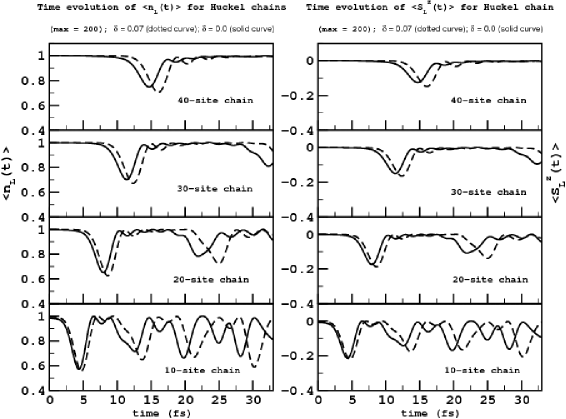
Figure 2: Time evolution of $\langle n_{L}(t)\rangle$ (Left) and $\langle S^{z}_{L}(t)\rangle$ (Right) for uniform (solid curve) and dimerized (dashed curve) Húckel chains of length 10, 20, 30 and 40 sites. 200 DMEV states per block is used.

4.2 Dynamics in Hubbard Chains:

Figs. 3, 4, and 5 gives the time evolution profiles of charge and spin densities at the last site of Hubbard chains for different chain lengths, and for several representative values of U, namely, U/t = 2.0, 4.0, and 6.0, respectively. It is observed that the charge and spin dynamics are no longer identical as was seen in case of Hückel chains clearly indicating spin-charge separation. Furthermore, as the magnitude of U increases, the extent of spin-charge decoupling also increases. In the literature, the decoupled spin and charge excitations are referred to as spinons, and holons kivelson , zou . For a given U/t, ”velocity” of the charge excitation (holon) as well as that of the spin excitation (spinon) seem to be weakly dependent on the chain length. It is however that at all chain lengths and nonzero U/t values, ”velocity” of the holon is higher than that of the spinon. If one examines the plots carefully, another interesting observation can be made; in the correlated models, dimerization plays little or no role in influencing the ”velocity” of the injected hole. Figs. 6 and 7, show the variation of $\langle n_{L}(\tau)\rangle$ and $\langle S_{L}^{z}(\tau)\rangle$ for regular and dimerized chains of given length, for different values of U. Solid curves are for U = 2.0, dashed curves represents U = 4.0, while U = 6.0 is depicted by dotted curves. It is observed that for a fixed chain length, increasing U, does not perceptibly affect the velocity of the holon appreciably, but spinon’s velocity is considerably altered. This is simply because, in case of the 1-dimensional Hubbard model, analytical expressions for the holon ($v_{h}$) and spinon ($v_{s}$) velocities are given by karen1 , coll ,

$$v_{h}=2t\sin{(\pi n)};~{}~{}v_{s}=\frac{2\pi t^{2}}{U}\biggl{[}1-\frac{\sin{(2\pi n)}}{2\pi n}\biggr{]}$$ (21)

where, $t$ and U are the nn hopping matrix element and the one-site Coulomb repulsion term, respectively, and $n$ is the particle density (n $\leq$ 1). Clearly, the velocity of the holon does not depend on U, while that of the spinon decreases, as established also from our tdDMRG studies. Furthermore, as U $\rightarrow\infty$, spin velocity goes to zero. The holon moves by virtue of the hopping matrix element while the effective spin-spin exchange, which is of the order of $\frac{t^{2}}{U}$, propagates the spinon. And, in the thermodynamic limit, that is, U $\rightarrow\infty$ limit, only the holon propagates, the spinon doesn’t ”move” at all, $v_{s}$ being zero. As the magnitude of U increases, the velocity of the spinon decreases.

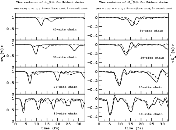
Figure 3: Time evolution of $\langle n_{L}(t)\rangle$ (Left) and $\langle S^{z}_{L}(t)\rangle$ (Right) for uniform (solid curve) and dimerized (dashed curve) Hubbard chains of length 10, 20, 30 and 40 sites, with $\frac{U}{\mid t\mid}$ = 2.0. Dimension of the DMEV basis used is 200.

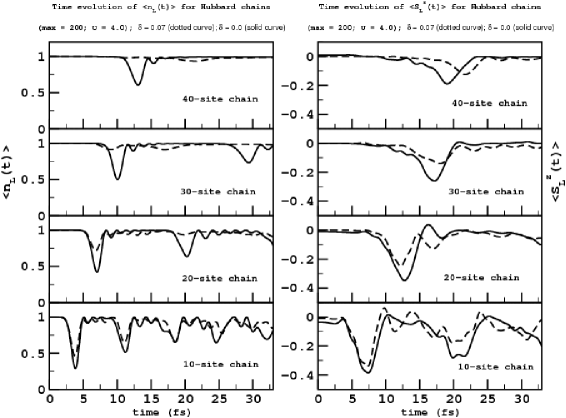
Figure 4: Time evolution of $\langle n_{L}(t)\rangle$ (Left) and $\langle S^{z}_{L}(t)\rangle$ (Right) for uniform (solid curve) and dimerized (dashed curve) Hubbard chains of length 10, 20, 30 and 40 sites, with $\frac{U}{\mid t\mid}$ = 4.0. Dimension of the DMEV basis used is 200.

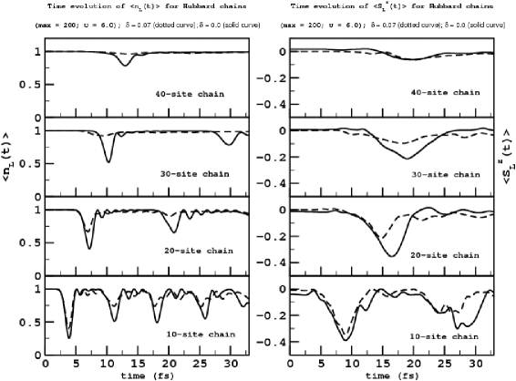
Figure 5: Time evolution of $\langle n_{L}(t)\rangle$ (Left) and $\langle S^{z}_{L}(t)\rangle$ (Right) for uniform (solid curve) and dimerized (dashed curve) Hubbard chains of length 10, 20, 30 and 40 sites, with $\frac{U}{\mid t\mid}$ = 6.0. Dimension of the DMEV basis used is 200.

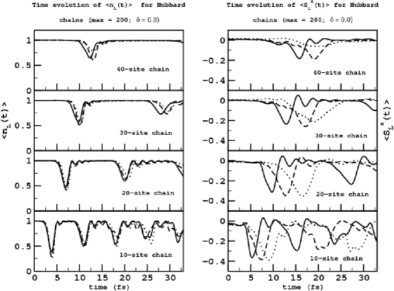
Figure 6: Comparison of the time evolutions of $\langle n_{L}(t)\rangle$ (Left) and $\langle S^{z}_{L}(t)\rangle$ (Right) for uniform Hubbard chains of length 10, 20, 30 and 40 sites, with $\frac{U}{\mid t\mid}$ = 2.0 (solid curve), 4.0 (dashed curve) and 6.0 (dotted curve). Dimension of the DMEV basis used is 200.

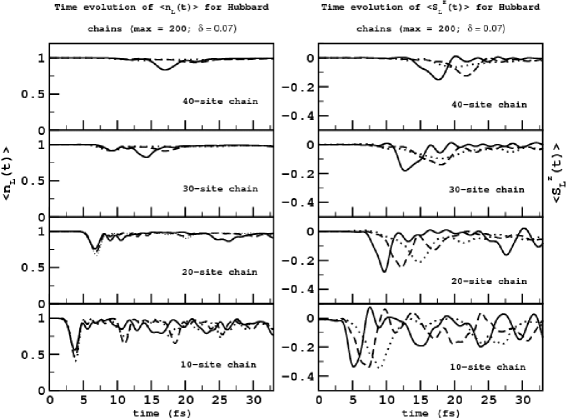
Figure 7: Comparison of the time evolutions of $\langle n_{L}(t)\rangle$ (Left) and $\langle S^{z}_{L}(t)\rangle$ (Right) for dimerized Hubbard chains ($\delta$ = 0.07) of length 10, 20, 30 and 40 sites, with $\frac{U}{\mid t\mid}$ = 2.0 (solid curve), 4.0 (dashed curve) and 6.0 (dotted curve). Dimension of the DMEV basis used is 200.

5 Summary and Outlook

To summarize, we find from our tdDMRG calculations that when a hole with a desired spin is injected at one end of the $\pi$-conjugated backbone of a polyene chain, it propagates from one end of the chain, to the other. The motion of this hole can be monitored by focusing our attention on the time evolution of the charge and spin densities at the two end-sites of the chain. In the absence of any external reservoirs (source-drain), the hole gets reflected back and forth across the length of the chain showing oscillatory motion. In the absence of electron-electron correlations, the charge and spin degrees of the hole do not get decoupled. The time taken by the hole to travel across the whole polyene backbone increases with approximately constant velocity. We are currently extending these studies to PPP model and polymer topologies involving phenyl rings. It is seen that for dimerized chains, the velocity decreases further because of the fact that velocity of the hole is determined by the smaller of the two hopping matrix element, $t_{i,i+1}=t_{0}(1-(\delta)^{i})$, where $\delta$ is the dimerization parameter and $t_{0}$ is the mean hopping matrix element. For Hubbard chains, where spin-charge separation occurs, the hole ”breaks-up” into two elementary excitations, one carrying only charge (holon), and the other, only spin (spinon), both of which moves with different velocities. It is found in accordance with the earlier literature, the holon moves faster than the spinon, and with increasing U, although the velocity of the holon remains ”almost” unaltered, that of the spinon significantly decreases.

Acknowledgment This work was supported by grants from the department of science and technology (DST), India.

References

- [1] A. Dodabalapur, L. Torsi, H.E. Katz, Science, 268 , 270 (1995).
- [2] A. Dodabalapur, H.E. Katz, L. Torsi, R.C. Haddon, Science, 269, 1560 (1995).
- [3] J.H. Burroughes, D.D.C. Bradeley, A.R. Brown, R.N. Marks, K. Machay, R.H. Friend, P.L. Burns, A.B. Holmes, Nature (London), 347, 539 (1990).
- [4] A. Nitzan and M. A. Ratner, Science, 300, 1384 (2003).
- [5] J. Rammer, and H. Smith, Rev. Mod. Phys., 58, 323-359 (2002).
- [6] S.R. White, Phys. Rev. Letters, 69, 2863 (1992).
- [7] S.R. White, Phys. Rev. B, 48, 10345 (1993).
- [8] I. Peschel, X. Wang, M. Kaulke, and K. Hallberg, Density Matrix Renormalization: A New Numerical Method in Physics, Springer Verlag, Berlin, (1999).
- [9] U. Schollwöck, J. Phys. Soc. Jpn., 74, 246 (2005); cond-mat/0409292 (2004); Rev. Mod. Phys., 77, 259 (2005).
- [10] S.R. White, and A.E. Feiguin, Phys. Rev. Letters., 93, 076401 (2004).
- [11] K. Hallberg, cond-mat/0303557, (2003).
- [12] E. Hückel, Z. Physik, 70, 204 (1931); 76, 628 (1932).
- [13] L. Salem, Molecular Orbital Theory of Conjugated Systems, Benjamin, New York, (1966).
- [14] J. Kanamori, Prog. Theor. Phys., 30, 275 (1963).
- [15] M.C. Gutzwiller, Phys. Rev. Letters, 10, 159 (1963).
- [16] J. Hubbard, Proc. Roc. Soc. (London), A276, 238 (1963).
- [17] R. Pariser, and R.G. Parr, J. Chem. Phys., 21, 466 (1953).
- [18] J.A. Pople, Trans. Farad. Soc., 49, 1375 (1953).
- [19] P.R. Surjan, Second Quantized Approach to Quantum Chemistry, Springer-Verlag, (1989).
- [20] K. Ohno, Theor. Chem. Acta., 2, 219 (1964); G. Klopman, J. Am. Chem. Soc., 86, 4550 (1964).
- [21] N. Mataga, and K. Nishimoto, Z. Physik. Chem., 12, 335 (1957); 13, 140 (1957).
- [22] J. Crank, and P. Nicholson, Proc. Cambridge. Philos. Soc., 43, 50 (1947).
- [23] A. Askar, and A.S. Cakmak, J. Chem. Phys., 68, 2794 (1978).
- [24] T. Iitaka, Phys. Rev. E, 49, 4684 (1994).
- [25] T. Dutta, and S. Ramasesha, unpublished.
- [26] H.G. Luo, T. Xiang, and X.Q. Wang, Phys. Rev. Letters., 91, 049701 (2003).
- [27] S.R. Manmana, A. Muramatsu, and R.M. Noack, cond-mat/0502396 (2005).
- [28] M. Cazalilla, and J.B. Marston, Phys. Rev. Letters., 88, 256403 (2002).
- [29] A.J. Daley, C. Kollath, U. Schollwöck, and G. Vidal, J. Stat. Mech.: Theor. Exp. , P04005 (2004).
- [30] G. Vidal, Phys. Rev. Letters., 91, 147902 (2003).
- [31] G. Vidal, Phys. Rev. Letters., 93, 040502 (2004).
- [32] S. Kivelson, D. Rokhsar, and J. Sethna, Phys. Rev. B, 35, 8865 (1987).
- [33] Z. Zou, and P.W. Anderson, Phys. Rev. B, 37, 627 (1998).
- [34] E.A. Jagla, K. Hallberg, and C.A. Balseiro, Phys. Rev. B, 47, 5849 (1993).
- [35] C.F. Coll, Phys. Rev. B, 9, 2150 (1974).