On Column-restricted and Priority Covering Integer Programs

Abstract

In a column-restricted covering integer program (CCIP), all the non-zero entries of any column of the constraint matrix are equal. Such programs capture capacitated versions of covering problems. In this paper, we study the approximability of CCIPs, in particular, their relation to the integrality gaps of the underlying 0,1-CIP.

If the underlying 0,1-CIP has an integrality gap $O(\gamma)$, and assuming that the integrality gap of the priority version of the 0,1-CIP is $O(\omega)$, we give a factor $O(\gamma+\omega)$ approximation algorithm for the CCIP. Priority versions of 0,1-CIPs (PCIPs) naturally capture quality of service type constraints in a covering problem.

We investigate priority versions of the line (PLC) and the (rooted) tree cover (PTC) problems. Apart from being natural objects to study, these problems fall in a class of fundamental geometric covering problems. We bound the integrality of certain classes of this PCIP by a constant. Algorithmically, we give a polytime exact algorithm for PLC, show that the PTC problem is APX-hard, and give a factor $2$-approximation algorithm for it.

1 Introduction

In a 0,1-covering integer program (0,1-CIP, in short), we are given a constraint matrix $A\in\{0,1\}^{m\times n}$, demands $b\in\mathbb{Z}^{m}_{+}$, non-negative costs $c\in\mathbb{Z}_{+}^{n}$, and upper bounds $d\in\mathbb{Z}^{n}_{+}$, and the goal is to solve the following integer linear program (which we denote by $\mathtt{Cov}(A,b,c,d)$).

$$\min\{c^{T}x\,:\,Ax\geq b,0\leq x\leq d,x\mbox{ integer}\}.$$

Problems that can be expressed as 0,1-CIPs are essentially equivalent to set multi-cover problems, where sets correspond to columns and elements correspond to rows. This directly implies that 0,1-CIPs are rather well understood in terms of approximability: the class admits efficient $O(\log n)$ approximation algorithms and this is best possible unless $\text{NP}=\text{P}$. Nevertheless, in many cases one can get better approximations by exploiting the structure of matrix $A$. For example, it is well known that whenever $A$ is totally unimodular (TU)(e.g., see [19]), the canonical LP relaxation of a 0,1-CIP is integral; hence, the existence of efficient algorithms for solving linear programs immediately yields fast exact algorithms for such 0,1-CIPs as well.

While a number of general techniques have been developed for obtaining improved approximation algorithms for structured $0,1$-CIPs, not much is known for structured non-$0,1$ CIP instances. In this paper, we attempt to mitigate this problem, by studying the class of column-restricted covering integer programs (CCIPs), where all the non-zero entries of any column of the constraint matrix are equal. Such CIPs arise naturally out of $0,1$-CIPs, and the main focus of this paper is to understand how the structure of the underlying 0,1-CIP can be used to derive improved approximation algorithms for CCIPs.

Column-Restricted Covering IPs (CCIPs): Given a 0,1-covering problem $\mathtt{Cov}(A,b,c,d)$ and a supply vector $s\in\mathbb{Z}^{n}_{+}$, the corresponding CCIP is obtained as follows. Let $A[s]$ be the matrix obtained by replacing all the $1$’s in the $j$th column by $s_{j}$; that is, $A[s]_{ij}=A_{ij}s_{j}$ for all $1\leq i\leq m,1\leq j\leq n$. The column-restricted covering problem is given by the following integer program.

$$\min\{c^{T}x\,:\,A[s]x\geq b,0\leq x\leq d,x\mbox{ integer}\}. \mathtt{Cov}(A[s],b,c,d)$$ ()

CCIPs naturally capture capacitated versions of 0,1-covering problems. To illustrate this we use the following 0,1-covering problem called the tree covering problem. The input is a tree $T=(V,E)$ rooted at a vertex $r\in V$, a set of segments ${\cal S}\subseteq\{(u,v):u\textrm{ is a child of}~{}v\}$, non-negative costs $c_{j}$ for all $j\in\mathcal{S}$, and demands $b_{e}\in\mathbb{Z}_{+}$ for all $e\in E$. An edge $e$ is contained in a segment $j=(u,v)$ if $e$ lies on the unique $u,v$-path in $T$. The goal is to find a minimum-cost subset $C$ of segments such that each edge $e\in E$ is contained in at least $b_{e}$ segments of $C$. When $T$ is just a line, we call the above problem, the line cover (LC) problem. In this example, the constraint matrix $A$ has a row for each edge of the tree and a column for each segment in $\mathcal{S}$. It is not too hard to show that this matrix is TU and thus these can be solved exactly in polynomial time.

In the above tree cover problem, suppose each segment $j\in\mathcal{S}$ also has a capacity supply $s_{j}$ associated with it, and call an edge $e$ covered by a collection of segments $C$ iff the total supply of the segments containing $e$ exceeds the demand of $e$. The problem of finding the minimum cost subset of segments covering every edge is precisely the column-restricted tree cover problem. The column-restricted line cover problem encodes the minimum knapsack problem and is thus NP-hard.

For general CIPs, the best known approximation algorithm, due to Kolliopoulos and Young [16], has a performance guarantee of $O(1+\log\alpha)$, where $\alpha$, called the dilation of the instance, denotes the maximum number of non-zero entries in any column of the constraint matrix. Nothing better is known for the special case of CCIPs unless one aims for bicriteria results where solutions violate the upper bound constraints $x\leq d$ (see Section 1.1 for more details).

In this paper, our main aim is to understand how the approximability of a given CCIP instance is determined by the structure of the underlying $0,1$-CIP. In particular, if a $0,1$-CIP has a constant integrality gap, under what circumstances can one get constant factor approximation for the corresponding CCIP? We make some steps toward finding an answer to this question.

In our main result, we show that there is a constant factor approximation algorithm for CCIP if two induced $0,1$-CIPs have constant integrality gap. The first is the underlying original 0,1-CIP. The second is a priority version of the 0,1-CIP (PCIP, in short), whose constraint matrix is derived from that of the 0,1-CIP as follows.

Priority versions of Covering IPs (PCIPs): Given a 0,1-covering problem $\mathtt{Cov}(A,b,c,d)$, a priority supply vector $s\in\mathbb{Z}_{+}^{n}$, and a priority demand vector $\pi\in\mathbb{Z}^{m}_{+}$, the corresponding PCIP is as follows. Define $A[s,\pi]$ to be the following 0,1 matrix

$$A[s,\pi]_{ij}=\left\{\begin{array}[]{l@{\quad:\quad}l}1&A_{ij}=1\mbox{ and }s_{j}\geq\pi_{i}\\ 0&\mbox{otherwise,}\end{array}\right.$$ (1)

Thus, a column $j$ covers row $i$, only if its priority supply is higher than the priority demand of row $i$. The priority covering problem is now as follows.

$$\min\{c^{T}x\,:\,A[s,\pi]x\geq\mathds{1},0\leq x\leq d,x\mbox{ integer}\}. \mathtt{Cov}(A[s,\pi],\mathds{1},c)$$ ()

We believe that priority covering problems are interesting in their own right, and they arise quite naturally in covering applications where one wants to model quality of service (QoS) or priority restrictions. For instance, in the tree cover problem defined above, suppose each segment $j$ has a quality of service (QoS) or priority supply $s_{j}$ associated with it and suppose each edge $e$ has a QoS or priority demand $\pi_{e}$ associated with it. We say that a segment $j$ covers $e$ iff $j$ contains $e$ and the priority supply of $j$ exceeds the priority demand of $e$. The goal is to find a minimum cost subset of segments that covers every edge. This is the priority tree cover problem.

Besides being a natural covering problem to study, we show that the priority tree cover problem is a special case of a classical geometric covering problem: that of finding a minimum cost cover of points by axis-parallel rectangles in $3$ dimensions. Finding a constant factor approximation algorithm for this problem, even when the rectangles have uniform cost, is a long standing open problem.

We show that although the tree cover is polynomial time solvable, the priority tree cover problem is APX-hard. We complement this with a factor $2$ approximation for the problem. Furthermore, we present constant upper bounds for the integrality gap of this PCIP in a number of special cases, implying constant upper bounds on the corresponding CCIPs in these special cases. We refer the reader to Section 1.2 for a formal statement of our results, which we give after summarizing works related to our paper.

1.1 Related work

There is a rich and long line of work ([10, 12, 18, 20, 21]) on approximation algorithms for CIPs, of which we state the most relevant to our work. Assuming no upper bounds on the variables, Srinivasan [20] gave a $O(1+\log\alpha)$-approximation to the problem (where $\alpha$ is the dilation as before). Later on, Kolliopoulos and Young [16] obtained the same approximation factor, respecting the upper bounds. However, these algorithms didn’t give any better results when special structure of the constraint matrix was known. On the hardness side, Trevisan [22] showed that it is NP-hard to obtain a $(\log\alpha-O(\log\log\alpha))$-approximation algorithm even for 0,1-CIPs.

The most relevant work to this paper is that of Kolliopoulos [13]. The author studies CCIPs which satisfy a rather strong assumption, called the no bottleneck assumption, that the supply of any column is smaller than the demand of any row. Kolliopoulos [13] shows that if one is allowed to violate the upper bounds by a multiplicative constant, then the integrality gap of the CCIP is within a constant factor of that of the original 0,1-CIP. As the author notes such a violation is necessary; otherwise the CCIP has unbounded integrality gap. If one is not allowed to violated upper bounds, nothing better than the result of [16] is known for the special case of CCIPs.

Our work on CCIPs parallels a large body of work on column-restricted packing integer programs (CPIPs). Assuming the no-bottleneck assumption, Kolliopoulos and Stein [15] show that CPIPs can be approximated asymptotically as well as the corresponding 0,1-PIPs. Chekuri et al. [7] subsequently improve the constants in the result from [15]. These results imply constant factor approximations for the column-restricted tree packing problem under the no-bottleneck assumption. Without the no-bottleneck assumption, however, only polylogarithmic approximation is known for the problem [6].

The only work on priority versions of covering problems that we are aware of is due to Charikar, Naor and Schieber [5] who studied the priority Steiner tree and forest problems in the context of QoS management in a network multicasting application. Charikar et al. present a $O(\log n)$-approximation algorithm for the problem, and Chuzhoy et al. [9] later show that no efficient $o(\log\log n)$ approximation algorithm can exist unless $\text{NP}\subseteq\text{DTIME}(n^{\log\log\log n})$ ($n$ is the number of vertices).

To the best of our knowledge, the column-restricted or priority versions of the line and tree cover problem have not been studied. The best known approximation algorithm known for both is the $O(\log n)$ factor implied by the results of [16] stated above. However, upon completion of our work, Nitish Korula [17] pointed out to us that a $4$-approximation for column-restricted line cover is implicit in a result of Bar-Noy et al. [2]. We remark that their algorithm is not LP-based, although our general result on CCIPs is.

1.2 Technical Contributions and Formal Statement of Results

Given a 0,1-CIP $\mathtt{Cov}(A,b,c,d)$, we obtain its canonical LP relaxation by removing the integrality constraint. The integrality gap of the CIP is defined as the supremum of the ratio of optimal IP value to optimal LP value, taken over all non-negative integral vectors $b,c$, and $d$. The integrality gap of an IP captures how much the integrality constraint affects the optimum, and is an indicator of the strength of a linear programming formulation.

CCIPs: Suppose the CCIP is $\mathtt{Cov}(A[s],b,c,d)$. We make the following two assumptions about the integrality gaps of the 0,1 covering programs, both the original 0,1-CIP and the priority version of the 0,1-CIP.

Assumption 1.

The integrality gap of the original 0,1-CIP is $\gamma\geq 1$. Specifically, for any non-negative integral vectors $b,c$, and $d$, if the canonical LP relaxation to the CIP has a fractional solution $x$, then one can find in polynomial time an integral feasible solution to the CIP of cost at most $\gamma\cdot c^{T}x$. We stress here that the entries of $b,c,d$ could be $0$ as well as $\infty$.

Assumption 2.

The integrality gap of the PCIP is $\omega\geq 1$. Specifically, for any non-negative integral vectors $s,\pi,c$, if the canonical LP relaxation to the PCIP has a fractional solution $x$, then one can find in polynomial time, an integral feasible solution to the PCIP of cost at most $\omega\cdot c^{T}x$.

We give an LP-based approximation algorithm for solving CCIPs. Since the canonical LP relaxation of a CCIP can have unbounded integrality gap, we strengthen it by adding a set of valid constraints called the knapsack cover constraints. We show that the integrality gap of this strengthened LP is $O(\gamma+\omega)$, and can be used to give a polynomial time approximation algorithm.

Theorem 1.

Under Assumptions 1 and 2, there is a $(24\gamma+8\omega)$-approximation algorithm for column-restricted CIPs.

Knapsack cover constraints to strengthen LP relaxations were introduced in [1, 11, 23]; Carr et al. [4] were the first to employ them in the design approximation algorithms. The paper of Kolliopoulos and Young [16] also use these to get their result on general CIPs.

The main technique in the design of algorithms for column-restricted problems is grouping-and-scaling developed by Kolliopoulos and Stein [14, 15] for packing problems, and later used by Kolliopoulos [13] in the covering context. In this technique, the columns of the matrix are divided into groups of ‘close-by’ supply values; in a single group, the supply values are then scaled to be the same; for a single group, the integrality gap of the original 0,1-CIP is invoked to get an integral solution for that group; the final solution is a ‘union’ of the solutions over all groups.

There are two issues in applying the technique to the new strengthened LP relaxation of our problem. Firstly, although the original constraint matrix is column-restricted, the new constraint matrix with the knapsack cover constraints is not. Secondly, unless additional assumptions are made, the current grouping-and-scaling analysis doesn’t give a handle on the degree of violation of the upper bound constraints. This is the reason why Kolliopoulos [13] needs the strong no-bottleneck assumption.

We get around the first difficulty by grouping the rows as well, into those that get most of their coverage from columns not affected by the knapsack constraints, and the remainder. On the first group of rows, we apply a subtle modification to the vanilla grouping-and-scaling analysis and obtain a $O(\gamma)$ approximate feasible solution satisfying these rows; we then show that one can treat the remainder of the rows as a PCIP and get a $O(\omega)$ approximate feasible solution satisfying them, using Assumption 2. Combining the two gives the $O(\gamma+\omega)$ factor. The full details are given in Section 2.

We stress here that apart from the integrality gap assumptions on the 0,1-CIPs, we do not make any other assumption (like the no-bottleneck assumption). In fact, we can use the modified analysis of the grouping-and-scaling technique to get a similar result as [13] for approximating CCIPs violating the upper-bound constraints, under a weaker assumption than the no-bottleneck assumption. The no-bottleneck assumption states that the supply of any column is less than the demand of any row. In particular, even though a column has entry $0$ on a certain row, its supply needs to be less than the demand of that row. We show that if we weaken the no-bottleneck assumption to assuming that the supply of a column $j$ is less than the demand of any row $i$ only if $A[s]_{ij}$ is positive, a similar result can be obtained via our modified analysis.

Theorem 2.

Under assumption 1 and assuming $A_{ij}s_{j}\leq b_{i}$, for all $i,j$, given a fractional solution $x$ to the canonical LP relaxation of $\mathtt{Cov}(A[s],b,c,d)$, one can find an integral solution $x^{\tt int}$ whose cost $c\cdot x^{\tt int}\leq 10\gamma(c\cdot x)$ and $x^{\tt int}\leq 10d$.

Priority Covering Problems.

In the following, we use PLC and PTC to refer to the priority versions of the line cover and tree cover problems, respectively. Recall that the constraint matrices for line and tree cover problems are totally unimodular, and the integrality of the corresponding 0,1-covering problems is therefore $1$ in both case. It is interesting to note that the 0,1-coefficient matrices for PLC and PTC are not totally unimodular in general. The following integrality gap bound is obtained via a primal-dual algorithm.

Theorem 3.

The canonical LP for priority line cover has an integrality gap of at least $3/2$ and at most $2$.

In the case of tree cover, we obtain constant upper bounds on the integrality gap for the case $c=\mathds{1}$, that is, for the minimum cardinality version of the problem. We believe that the PCIP for the tree cover problem with general costs also has a constant integrality gap. On the negative side, we can show an integrality gap of at least $\frac{e}{e-1}$.

Theorem 4.

The canonical LP for unweighted PTC has an integrality gap of at most $6$.

We obtain the upper bound by taking a given PTC instance and a fractional solution to its canonical LP, and decomposing it into a collection of PLC instances with corresponding fractional solutions, with the following two properties. First, the total cost of the fractional solutions of the PLC instances is within a constant of the cost of the fractional solution of the PTC instance. Second, union of integral solutions to the PLC instances gives an integral solution to the PTC instance. The upper bound follows from Theorem 3. Using Theorem 1, we get the following as an immediate corollary.

Corollary 1.

There are $O(1)$-approximation algorithms for column-restricted line cover and the cardinality version of the column-restricted tree cover.

We also obtain the following combinatorial results.

Theorem 5.

There is a polynomial-time exact algorithm for PLC.

Theorem 6.

PTC is APX-hard, even when all the costs are unit.

Theorem 7.

There is an efficient $2$-approximation algorithm for PTC.

The algorithm for PLC is a non-trivial dynamic programming approach that makes use of various structural observations about the optimal solution. The approximation algorithm for PTC is obtained via a similar decomposition used to prove Theorem 4.

We end by noting some interesting connections between the priority tree covering problem and set covering problems in computational geometry. The rectangle cover problem in $3$-dimensions is the following: given a collection of points $P$ in $\mathbb{R}^{3}$, and a collection $C$ of axis-parallel rectangles with costs, find a minimum cost collection of rectangles that covers every point. We believe studying the PTC problem could give new insights into the rectangle cover problem.

Theorem 8.

The priority tree covering problem is a special case of the rectangle cover problem in $3$-dimensions.

2 General Framework for Column Restricted CIPs

In this section we prove Theorem 1. Our goal is to round a solution to a LP relaxation of $\mathtt{Cov}(A[s],b,c,d)$ into an approximate integral solution. We strengthen the following canonical LP relaxation of the CCIP

$$\min\{c^{T}x~{}:~{}A[s]x\geq b,0\leq x\leq d,x\geq 0\}$$

by adding valid knapsack cover constraints. In the following we use $\mathcal{C}$ for the set of columns and $\mathcal{R}$ for the set of rows of $A$.

2.1 Strengthening the canonical LP Relaxation

Let $F\subset\mathcal{C}$ be a subset of the columns in the column restricted CIP $\mathtt{Cov}(A[s],b,c,d)$. For all rows $i\in\mathcal{R}$, define $b^{F}_{i}=\max\{0,b_{i}-\sum_{j\in F}A[s]_{ij}d_{j}\}$ to be the residual demand of row $i$ w.r.t. $F$. Define matrix $A^{F}[s]$ by letting

$$A^{F}[s]_{ij}=\left\{\begin{array}[]{l@{\quad:\quad}l}\min\{A[s]_{ij},b^{F}_{i}\}&j\in\mathcal{C}\setminus F\\ 0&j\in F,\end{array}\right.$$ (2)

for all $i\in\mathcal{C}$ and for all $j\in\mathcal{R}$. The following Knapsack-Cover (KC) inequality

$$\sum_{j\in\mathcal{C}}A^{F}[s]_{ij}x_{j}\geq b^{F}_{i}$$

is valid for the set of all integer solutions $x$ for $\mathtt{Cov}(A[s],b,c,d)$. Adding the set of all KC inequalities yields the following stronger LP formulation CIP. We note that the LP is not column-restricted, in that, different values appear on the same column of the new constraint matrix.

$$\mathtt{opt}_{P}:=\min\quad \sum_{j\in\mathcal{C}}c_{j}x_{j}$$ (P)

s.t. $$\sum_{j\in\mathcal{C}}A^{F}[s]_{ij}x_{j}\geq b^{F}_{i}\quad \forall F\subseteq\mathcal{C},\forall i\in\mathcal{R}$$ (3)

$$0\leq x_{j}\leq d_{j} \forall j\in\mathcal{C}$$

It is not known whether (P) can be solved in polynomial time. For $\alpha\in(0,1)$, call a vector $x^{*}$ $\alpha$-relaxed if its cost is at most $\mathtt{opt}_{P}$, and if it satisfies (3) for $F=\{j\in\mathcal{C}\,:\,x^{*}_{j}\geq\alpha d_{j}\}$. An $\alpha$-relaxed solution to (P) can be computed efficiently for any $\alpha$. To see this note that one can check whether a candidate solution satisfies (3) for a set $F$; we are done if it does, and otherwise we have found an inequality of (P) that is violated, and we can make progress via the ellipsoid method. Details can be found in [4] and [16].

We fix an $\alpha\in(0,1)$, specifying its precise value later. Compute an $\alpha$-relaxed solution, $x^{*}$, for (P), and let $F=\{j\in\mathcal{C}\,:\,x^{*}_{j}\geq\alpha d_{j}\}$. Define $\bar{x}$ as, $\bar{x}_{j}=x^{*}_{j}$ if $j\in\mathcal{C}\setminus F$, and $\bar{x}_{j}=0$, otherwise. Since $x^{*}$ is an $\alpha$-relaxed solution, we get that $\bar{x}$ is a feasible fractional solution to the residual CIP, $\mathtt{Cov}(A^{F}[s],b^{F},c,\alpha d)$. In the next subsection, our goal will be to obtain an integral feasible solution to the covering problem $\mathtt{Cov}(A^{F}[s],b^{F},c,d)$ using $\bar{x}$. The next lemma shows how this implies an approximation to our original CIP.

Lemma 1.

If there exists an integral feasible solution, $x^{\tt int}$, to $\mathtt{Cov}(A^{F}[s],b^{F},c,d)$ with $c^{T}x^{\tt int}\leq\beta\cdot c^{T}\bar{x}$, then there exists a $\max\{1/\alpha,\beta\}$-factor approximation to $\mathtt{Cov}(A[s],b,c,d)$.

Proof.

Define

$$z_{j}=\left\{\begin{array}[]{l@{\quad:\quad}l}d_{j}&j\in F\\ x^{\tt int}_{j}&j\in\mathcal{C}\setminus F,\end{array}\right.$$ (4)

Observe that $z\leq d$. $z$ is a feasible integral solution to $\mathtt{Cov}(A[s],b,c,d)$ since for any $i\in\mathcal{R}$,

$$\sum_{j\in\mathcal{C}}A[s]_{ij}z_{j}=\sum_{j\in F}A[s]_{ij}d_{j}+\sum_{j\in\mathcal{C}\setminus F}A[s]_{ij}x^{\tt int}_{j}\geq(b_{i}-b^{F}_{i})+\sum_{j\in\mathcal{C}\setminus F}A^{F}[s]_{ij}x^{\tt int}_{j}\geq b_{i}$$

where the first inequality follows from the definition of $b^{F}_{i}$ and since $A[s]_{ij}\geq A^{F}[s]_{ij}$, the second inequality follows since $x^{\tt int}$ is a feasible solution to $\mathtt{Cov}(A^{F}[s],b^{F},c,d)$.

Furthermore,

$$c^{T}z=\sum_{j\in F}c_{j}d_{j}+\sum_{j\in\mathcal{C}\setminus F}c_{j}x^{\tt int}_{j}\leq\frac{1}{\alpha}\sum_{j\in F}c_{j}x^{*}_{j}+\beta\sum_{j\in\mathcal{C}\setminus F}c_{j}x^{*}_{j}\leq\max\{\frac{1}{\alpha},\beta\}\mathtt{opt}_{P}$$

where the first inequality follows from the definition of $F$ and the second from the assumption in the theorem statement. ∎

2.2 Solving the Residual Problem

In this section we use a feasible fractional solution $\bar{x}$ of $\mathtt{Cov}(A^{F}[s],b^{F},c,\alpha d)$, to obtain an integral feasible solution $x^{\tt int}$ to the covering problem $\mathtt{Cov}(A^{F}[s],b^{F},c,d)$, with $c^{T}x^{\tt int}\leq\beta c^{T}\bar{x}$ for $\beta=24\gamma+8\omega$. Fix $\alpha=1/24$.

Converting to Powers of $2$. For ease of exposition, we first modify the input to the residual problem $\mathtt{Cov}(A^{F}[s],b^{F},c,d)$ so that all entries of are powers of $2$. For every $i\in\mathcal{R}$, let $\bar{b}_{i}$ denote the smallest power of $2$ larger than $b^{F}_{i}$. For every column $j\in\mathcal{C}$, let $\bar{s}_{j}$ denote the largest power of $2$ smaller than $s_{j}$.

Lemma 2.

$y=4\bar{x}$ is feasible for $\mathtt{Cov}(A^{F}[\bar{s}],\bar{b},c,4\alpha d)$.

Proof.

Focus on row $i\in\mathcal{R}$. We have

$$\sum_{j\in\mathcal{C}}A^{F}[\bar{s}]_{ij}y_{j}\geq 2\cdot\sum_{j\in\mathcal{C}}A^{F}[s]_{ij}\bar{x}_{j}\geq 2b^{F}_{i}\geq\bar{b}_{i},$$

where the first inequality uses the fact that $s_{j}\leq 2\bar{s}_{j}$ for all $j\in\mathcal{C}$, the second inequality uses the fact that $\bar{x}$ is feasible for $\mathtt{Cov}(A^{F}[s],b^{F},c,\alpha d)$, and the third follows from the definition of $\bar{b}_{i}$. ∎

Partitioning the rows. We call $\bar{b}_{i}$ the residual demand of row $i$. For a row $i$, a column $j\in\mathcal{C}$ is $i$-large if the supply of $j$ is at least the residual demand of row $i$; it is $i$-small otherwise. Formally,

$$\mathcal{L}_{i} = \{j\in\mathcal{C}\,:\,A_{ij}=1,\bar{s}_{j}\geq\bar{b}_{i}\}~{}~{}\mbox{ is the set of $i$-large columns}$$

$$\mathcal{S}_{i} = \{j\in\mathcal{C}\,:\,A_{ij}=1,\bar{s}_{j}<\bar{b}_{i}\}~{}~{}\mbox{ is the set of $i$-small columns}$$

Recall the definition from (2), $A^{F}[\bar{s}]_{ij}=\min(A[\bar{s}]_{ij},b^{F}_{i})$. Therefore, $A^{F}[\bar{s}]_{ij}=A_{ij}b^{F}_{i}$ for all $j\in\mathcal{L}_{i}$ since $\bar{s}_{j}\geq\bar{b}_{i}\geq b^{F}_{i}$; and $A^{F}[\bar{s}]_{ij}=A_{ij}\bar{s}_{j}$ for all $j\in\mathcal{S}_{i}$, since being powers of $2$, $\bar{s}_{j}<\bar{b}_{i}$ implies, $\bar{s}_{j}\leq\bar{b}_{i}/2\leq b^{F}_{i}$.

We now partition the rows into large and small depending on which columns most of their coverage comes from. Formally, call a row $i\in\mathcal{R}$ large if

$$\sum_{j\in\mathcal{S}_{i}}A^{F}[\bar{s}]_{ij}y_{j}\leq\sum_{j\in\mathcal{L}_{i}}A^{F}[\bar{s}]_{ij}y_{j},$$

and small otherwise. Note that Lemma 2 together with the fact that each column in row $i$’s support is either small or large implies,

$$\mbox{For a large row $i$,}~{}~{}\sum_{j\in\mathcal{L}_{i}}A^{F}[\bar{s}]_{ij}y_{j}\geq\bar{b}_{i}/2,~{}~{}\mbox{For a small row $i$,}~{}~{}\sum_{j\in\mathcal{S}_{i}}A^{F}[\bar{s}]_{ij}y_{j}\geq\bar{b}_{i}/2$$

Let $\mathcal{R}_{L}$ and $\mathcal{R}_{S}$ be the set of large and small rows.

In the following, we address small and large rows separately. We compute a pair of integral solutions $x^{{\tt int},\mathcal{S}}$ and $x^{{\tt int},\mathcal{L}}$ that are feasible for the small and large rows, respectively. We then obtain $x^{\tt int}$ by letting

$$x^{\tt int}_{j}=\max\{x^{{\tt int},\mathcal{S}}_{j},x^{{\tt int},\mathcal{L}}_{j}\},$$ (5)

for all $j\in\mathcal{C}$.

2.2.1 Small rows.

For these rows we use the grouping-and-scaling technique a la [7, 13, 14, 15]. However, as mentioned in the introduction, we use a modified analysis that bypasses the no-bottleneck assumptions made by earlier works.

Lemma 3.

We can find an integral solution $x^{{\tt int},\mathcal{S}}$ such that
a) $x^{{\tt int},\mathcal{S}}_{j}\leq d_{j}$ for all $j$,
b) $\sum_{j\in\mathcal{C}}c_{j}x^{{\tt int},\mathcal{S}}_{j}\leq 24\gamma\sum_{j\in\mathcal{C}}c_{j}\bar{x}_{j}$, and
c) for every small row $i\in\mathcal{R}_{S}$, $\sum_{j\in\mathcal{C}}A^{F}[s]_{ij}x^{{\tt int},\mathcal{S}}_{j}\geq b^{F}_{i}$.

Proof.

The complete proof is slightly technical and hence we start with a sketch. Since the rows are small, for any row $i$, we can zero out the entries that are larger than $\bar{b}_{i}$, and still $2y$ will be a feasible solution. Note that, now in each row, the entries are $<\bar{b}_{i}$, and thus are at most $\bar{b}_{i}/2$ (everything being powers of $2$). We stress that it could be that $\bar{b}_{i}$ of some row is less than the entry in some other row, that is, we don’t have the no-bottleneck assumption. However, when a particular row $i$ is fixed, $\bar{b}_{i}$ is at least any entry of the matrix in the $i$th row. Our modified analysis of grouping and scaling then makes the proof go through.

We group the columns into classes that have $s_{j}$ as the same power of $2$, and for each row $i$ we let $\bar{b}_{i}^{(t)}$ be the contribution of the class $t$ columns towards the demand of row $i$. The columns of class $t$, the small rows, and the demands $\bar{b}_{i}^{(t)}$ form a CIP where all non-zero entries of the matrix are the same power of $2$. We scale both the constraint matrix and $\bar{b}^{(t)}_{i}$ down by that power of $2$ to get a 0,1-CIP, and using assumption 1, we get an integral solution to this 0,1-CIP. Our final integral solution is obtained by concatenating all these integral solutions over all classes.

Till now the algorithm is the standard grouping-and-scaling algorithm. The difference lies in our analysis in proving that this integral solution is feasible for the original CCIP. Originally the no-bottleneck assumption was used to prove this. However, we show since the column values in different classes are geometrically decreasing, the weaker assumption of $\bar{b}_{i}$ being at least any entry in the $i$th row is enough to make the analysis go through. We now get into the full proof.

Step 1: Grouping the columns.

Let $\bar{s}_{min}$ and $\bar{s}_{max}$ be the smallest and largest supply among the columns in $\mathcal{C}\setminus F$. Since all $\bar{s}_{j}$ are powers of $2$, we introduce the shorthand, $\bar{s}^{(t)}$ for the supply $\bar{s}_{\max}/2^{t}$. We say that a column $j$ is in class $t\geq 0$, if $\bar{s}_{j}=\bar{s}^{(t)}$, and we let

$$\mathcal{C}^{(t)}:=\{j\in\mathcal{C}\setminus F\,:\,\bar{s}_{j}=\bar{s}^{(t)}\}$$

be the set of class $t$ supplies.

Step 2: Disregarding $i$-large columns of a small row $i$.

Fix a small row $i\in\mathcal{R}_{S}$. We now identify the columns $j$ that are $i$-small. To do so, define $t_{i}:=\log(\bar{s}_{max}/\bar{b}_{i})+1$. Observe that any column $j$ in class $\mathcal{C}^{(t)}$ for $t\geq t_{i}$ are $i$-small. This is because $\bar{s}_{j}=s_{max}/2^{t}\leq s_{max}/2^{t_{i}}=\bar{b}_{i}/2<\bar{b}_{i}$. Define

$$\bar{b}^{(t)}_{i}=\left\{\begin{array}[]{l@{\quad: \quad}l}2\sum_{j\in\mathcal{C}^{(t)}}A^{F}[\bar{s}]_{ij}y_{j}&t\geq t_{i}\\ 0&\mbox{otherwise}\end{array}\right.$$

as the contribution of the class $t$, $i$-small columns to the demand of row $i$, multiplied by $2$. Note that by definition of small rows, these columns contribute to more than $1/2$ of the demand, and so

$$\sum_{t\geq t_{i}}\bar{b}^{(t)}_{i}\geq\bar{b}_{i}.$$ (6)

Henceforth, we will consider only the contributions of the small $i$-columns of a small row $i$.

Step 3: Scaling and getting the integral solution.

Fix a class $t$ of columns and scale down by $\bar{s}^{(t)}$ to get a $\{0,1\}$-constraint matrix. (Recall entries of the columns in a class $t$ are all $\bar{s}^{(t)}$.) This will enable us to apply assumption $1$ and get a integral solution corresponding to these columns. The final integral solution will be the concatenation of the integral solutions over the various classes.

The constants in the next claim are carefully chosen for the calculations to work out later.

Claim 1.

For any $t\geq 0$ and for all $i\in\mathcal{R}_{S}$, $6\cdot\sum_{j\in\mathcal{C}^{(t)}}A_{ij}y_{j}\geq\lfloor 3\bar{b}^{(t)}_{i}/\bar{s}^{(t)}\rfloor$.

Proof.

The claim is trivially true for rows $i$ with $t_{i}>t$ as $\bar{b}^{(t)}_{i}=0$ in this case. Consider a row $i$ with $t_{i}\leq t$. Since any column $j\in\mathcal{C}^{(t)}$ is $i$-small, we get $A^{F}[\bar{s}]_{ij}=A_{ij}\bar{s}_{j}=A_{ij}\bar{s}^{(t)}$. Using the definition of $\bar{b}_{i}$, we obtain

$$6\cdot\sum_{j\in\mathcal{C}^{(t)}}A_{ij}\bar{s}^{(t)}y_{j}=3\bar{b}^{(t)}_{i}.$$

Dividing both sides by $\bar{s}^{(t)}$ and taking the floor on the right-hand side yields the claim. ∎

Since $\alpha=1/24$ and $\bar{x}$ is a feasible solution to $\mathtt{Cov}(A^{F}[s],b^{F},c,d/24)$, we get that $6y_{j}=24\cdot\bar{x}_{j}\leq d_{j}$ for all $j\in\mathcal{C}\setminus F$. Thus, the above claim shows that $6y$ is a feasible fractional solution for $\mathtt{Cov}(A^{(t)},\lfloor 3\bar{b}^{(t)}/\bar{s}^{(t)}\rfloor,c^{(t)},d^{(t)})$, where $A^{(t)}$ is the submatrix of $A$ defined by the columns in $\mathcal{C}^{(t)}$, and $c^{(t)}$ and $d^{(t)}$ are the sub-vectors of $c$ and $d$, respectively, that are induced by $\mathcal{C}^{(t)}$. Using Assumption 1, we therefore conclude that there is an integral vector $x^{{\tt int},\mathcal{S},t}$ such that

$$x^{{\tt int},\mathcal{S},t}_{j} \leq d_{j}\quad\mbox{for all $j\in\mathcal{C}^{(t)}$, and}$$ (7)

$$\sum_{j\in\mathcal{C}^{(t)}}A^{(t)}_{ij}x^{{\tt int},\mathcal{S},t}_{j} \geq \left\lfloor\frac{3\bar{b}^{(t)}_{i}}{\bar{s}^{(t)}}\right\rfloor\quad\mbox{for all $i\in\mathcal{R}_{S}$, and}$$ (8)

$$\sum_{j\in\mathcal{C}^{(t)}}c_{j}x^{{\tt int},\mathcal{S},t}_{j} \leq 6\gamma\cdot\sum_{j\in\mathcal{C}^{(t)}}c_{j}y_{j}$$ (9)

We obtain integral solution $x^{{\tt int},\mathcal{S}}$ by letting $x^{{\tt int},\mathcal{S}}_{j}=x^{{\tt int},\mathcal{S},t}_{j}$ if $j\in\mathcal{C}^{(t)}$. Thus $x^{{\tt int},\mathcal{S}}_{j}\leq d_{j}$ for all $j\in\mathcal{C}$, and we get,

$$\sum_{j\in\mathcal{C}}c_{j}x^{{\tt int},\mathcal{S}}_{j}=\sum_{t\geq 0}\sum_{j\in\mathcal{C}^{(t)}}c_{j}x^{{\tt int},\mathcal{S},t}_{j}\leq 6\gamma\cdot\sum_{t\geq 0}\sum_{j\in\mathcal{C}^{(t)}}c_{j}y_{j}=24\gamma\cdot\sum_{j\in\mathcal{C}}c_{j}\bar{x}_{j}.$$ (10)

Thus we have established parts (a) and (b) of the lemma. It remains to show that $x^{{\tt int},\mathcal{S}}$ is feasible for the set of small rows.

Step 4: Putting them all together: scaling back.

Once again, fix a small row $i\in\mathcal{R}_{S}$. The following inequality takes only contribution of the $i$-small columns. We later show this suffices.

$$\sum_{j\in\mathcal{C}}A^{F}[s]_{ij}x^{{\tt int},\mathcal{S}}_{j}\geq~{}~{}~{}~{}\sum_{j\in\mathcal{C}:~{}j\mbox{ is $i$-small}}A_{ij}s_{j}x^{{\tt int},\mathcal{S}}_{j}~{}~{}~{}~{}~{}~{}~{}~{}~{}~{}~{}~{}~{}~{}~{}~{}~{}~{}~{}~{}~{}~{}~{}~{}~{}~{}$$

$$=~{}~{}~{}\sum_{t\geq t_{i}}\sum_{j\in\mathcal{C}^{(t)}}A^{(t)}_{ij}s_{j}x^{{\tt int},\mathcal{S}}_{j}\geq\sum_{t\geq t_{i}}\sum_{j\in\mathcal{C}^{(t)}}A^{(t)}_{ij}\bar{s}^{(t)}x^{{\tt int},\mathcal{S},t}_{j}$$ (11)

The first inequality follows since $A^{F}[s]_{ij}=A_{ij}s_{j}$ for $i$-small columns, the equality follows from the definition of $t_{i}$, and the final inequality uses the fact that $s_{j}\geq\bar{s}^{(t)}$ for $j\in\mathcal{C}^{(t)}$. The following claim along with (2.2.1) proves feasibility of row $i$. This is the part where our analysis slightly differs from the standard grouping-and-scaling analysis.

Claim 2.

For any small row $i\in\mathcal{R}_{S}$,

$$\sum_{t\geq t_{i}}\sum_{j\in\mathcal{C}^{(t)}}A^{(t)}_{ij}\bar{s}^{(t)}x^{{\tt int},\mathcal{S},t}_{j}\geq b^{F}_{i}.$$

Proof.

In this proof, the choice of the constant $3$ on the right-hand side of the inequality in Claim 1 will become clear. Let $S_{i}=\{t\geq t_{i}\,:\,3\bar{b}^{(t)}_{i}<\bar{s}^{(t)}\}$ be the set of $i$-small classes $t$ whose fractional supply $\bar{b}^{(t)}_{i}$ is small compared to its integral supply $\bar{s}^{(t)}$. We now show that for any small row $i$, the columns in the classes not in $S_{i}$ suffice to satisfy its demand. Note that

$$\sum_{t\not\in S_{i},t\geq t_{i}}\bar{b}^{(t)}_{i}=\sum_{t\geq t_{i}}\bar{b}^{(t)}_{i}-\sum_{t\in S_{i}}\bar{b}^{(t)}_{i}\geq\sum_{t\geq t_{i}}\bar{b}^{(t)}_{i}-\frac{1}{3}\sum_{t\in S_{i}}\bar{s}^{(t)}$$ (12)

which follows from the definition of $S_{i}$. Furthermore, from (6) we know that for a small row, $\sum_{t\geq t_{i}}\bar{b}^{(t)}_{i}\geq\bar{b}_{i}$. Also, since $\bar{s}^{(t)}$ form a geometric series, we get that $\sum_{t\in S_{i}}\bar{s}^{(t)}\leq\sum_{t\geq t_{i}}\bar{s}^{(t)}\leq 2\bar{s}^{(t_{i})}$. Putting this in (12) we get

$$\sum_{t\not\in S_{i},t\geq t_{i}}\bar{b}^{(t)}_{i}\geq\bar{b}_{i}-\frac{1}{3}\sum_{t\geq t_{i}}\bar{s}^{(t)}\geq\bar{b}_{i}-\frac{2}{3}\bar{s}^{(t_{i})}=\frac{2}{3}\bar{b}_{i},$$ (13)

where the final equality follows from the definition of $t_{i}$ which implies that $\bar{s}^{(t_{i})}=\bar{b}_{i}/2$.

Moreover, for $t\not\in S_{i}$, we know that $\lfloor 3\bar{b}^{t}_{i}/\bar{s}^{(t)}\rfloor\geq\frac{3}{2}\bar{b}^{t}_{i}/\bar{s}^{(t)}$ since $\lfloor a\rfloor\geq a/2$ if $a>1$. Therefore, using inequality (8) in (2.2.1), we get

$$\sum_{j\in\mathcal{C}}A^{F}[s]_{ij}x^{{\tt int},\mathcal{S}}_{j}\geq\sum_{t\geq t_{i}}\sum_{j\in\mathcal{C}^{(t)}}A^{(t)}_{ij}\bar{s}^{(t)}x^{{\tt int},\mathcal{S},t}_{j} \geq \sum_{t\not\in S_{i},t\geq t_{i}}\bar{s}^{(t)}\left\lfloor\frac{3\bar{b}^{(t)}_{i}}{\bar{s}^{(t)}}\right\rfloor$$

$$\geq \frac{3}{2}\sum_{t\not\in S_{i},t\geq t_{i}}\bar{b}^{(t)}_{i}$$

$$\geq \bar{b}_{i}\geq b^{F}_{i},$$

where the second-last inequality uses (13), and the last uses the definition of $\bar{b}_{i}$. This completes the proof of the lemma. ∎

∎

2.2.2 Large rows.

The large rows can be showed to be a PCIP problem and thus Assumption 2 can be invoked to get an analogous lemma to Lemma 3.

Lemma 4.

We can find an integral solution $x^{{\tt int},\mathcal{L}}$ such that
a) $x^{{\tt int},\mathcal{L}}_{j}\leq 1$ for all $j$,
b) $\sum_{j\in\mathcal{C}}c_{j}x^{{\tt int},\mathcal{S}}_{j}\leq 8\omega\sum_{j\in\mathcal{C}}c_{j}\bar{x}_{j}$, and
c) for every large row $i\in\mathcal{R}_{L}$, $\sum_{j\in\mathcal{C}}A^{F}[s]_{ij}x^{{\tt int},\mathcal{S}}_{j}\geq b^{F}_{i}$.

Proof.

Let $i\in\mathcal{R}_{L}$ be a large row, and recall that $\mathcal{L}_{i}$ is the set of $i$-large columns in $\mathcal{C}$. We have

$$\sum_{j\in\mathcal{L}_{i}}A^{F}[s]_{ij}y_{j}=\sum_{j\in\mathcal{L}_{i}}A_{ij}\bar{b}_{i}y_{j}\geq\bar{b}_{i}/2,$$

and hence

$$2\sum_{j\in\mathcal{L}_{i}}A_{ij}y_{j}\geq 1.$$ (14)

Let $A^{\mathcal{R}}$ be the minor of $A$ induced by the large rows. Consider the priority cover problem $\mathtt{Cov}(A^{\mathcal{R}}[\bar{s},\bar{b}],\mathds{1},c)$. From the definition of $\mathcal{L}_{i}$, it follows $2y$ is a feasible fractional solution to the priority cover problem.

Using Assumption 2, we conclude that there is an integral solution $x^{{\tt int},\mathcal{L}}$ such that $\sum_{j\in\mathcal{C}}c_{j}x^{{\tt int},\mathcal{L}}_{j}\leq 2\omega\sum_{j\in\mathcal{C}}c_{j}y_{j}=8\omega\sum_{j\in\mathcal{C}}c_{j}\bar{x}_{j}$, and $\sum_{j\in\mathcal{C}}A^{\mathcal{R}}_{ij}x^{{\tt int},\mathcal{L}}_{j}\geq 1$, for all large rows $i\in\mathcal{R}_{L}$.

Fix a large row $i$. Since $A^{F}[s]_{ij}=b^{F}_{i}$ for all $i$-large columns $\mathcal{L}_{i}$, we get

$$\sum_{j\in\mathcal{C}}A^{F}[s]_{ij}x^{{\tt int},\mathcal{L}}_{j}\geq\sum_{j\in\mathcal{L}_{i}}A_{ij}b^{F}_{i}x^{{\tt int},\mathcal{L}}_{j}=b^{F}_{i}\sum_{j\in C}A^{\mathcal{R}}_{ij}x^{{\tt int},\mathcal{L}}_{j}\geq b^{F}_{i}$$

This completes the proof of the lemma. ∎

Proof of Theorem 1 Let $x^{{\tt int},\mathcal{S}}$ and $x^{{\tt int},\mathcal{L}}$ be as satisfying the conditions of Lemma 3 and 4, respectively. Define $x^{\tt int}$ as $x^{\tt int}_{j}=\max\{x^{{\tt int},\mathcal{S}}_{j},x^{{\tt int},\mathcal{L}}_{j}\}$. We have

a) $x^{\tt int}_{j}\leq d_{j}$ since both $x^{{\tt int},\mathcal{S}}_{j}\leq d_{j}$ and $x^{{\tt int},\mathcal{L}}_{j}\leq 1\leq d_{j}$.

b) For any row $i$, $\sum_{j\in\mathcal{C}}A^{F}[s]_{ij}x^{\tt int}_{j}\geq b^{F}_{i}$ since the inequality is true with $x^{\tt int}$ replaced by $x^{{\tt int},\mathcal{S}}$ for small rows, and $x^{\tt int}$ by $x^{{\tt int},\mathcal{L}}$ for large rows.

c) $\sum_{j\in\mathcal{C}}c_{j}x^{\tt int}_{j}\leq\sum_{j\in\mathcal{C}}c_{j}x^{{\tt int},\mathcal{S}}_{j}+\sum_{j\in\mathcal{C}}c_{j}x^{{\tt int},\mathcal{L}}_{j}\leq(24\gamma+8\omega)\sum_{j\in\mathcal{C}}c_{j}\bar{x}_{j}$.

Thus, $x^{\tt int}$ is a feasible integral solution to $\mathtt{Cov}(A^{F}[s],b^{F},c,d)$ with cost bounded as $\sum_{j\in\mathcal{C}}c_{j}x^{\tt int}_{j}\leq(24\gamma+8\omega)\sum_{j\in\mathcal{C}}c_{j}\bar{x}_{j}$. Noting that $\alpha=1/24$, the proof of the theorem follows from Lemma 1. $\square$.

2.3 CCIPs with violation of upper-bounds: Proof of Theorem 2

In this section we prove Theorem 2 that we restate here. In the proof, we will indicate how we modify the analysis of grouping-and-scaling that allows us to replace the no-bottleneck assumption with a weaker one.

Theorem 9.

(Theorem 2) Under assumption 1 and assuming $A_{ij}s_{j}\leq b_{i}$, for all $i,j$, given a fractional solution $x$ to the canonical LP relaxation of $\mathtt{Cov}(A[s],b,c,d)$, one can find an integral solution $x^{\tt int}$ whose cost $c\cdot x^{\tt int}\leq 10\gamma(c\cdot x)$ and $x^{\tt int}\leq 10d$.

Proof.

Let $x$ be a feasible solution to $A[s]x\geq b,x\geq 0$. We construct an integral solution $x^{\tt int}$ such that $A[s]x^{\tt int}\geq b$ and $c^{T}x^{\tt int}\leq 10\gamma c^{T}x$. Let $s_{max}$ and $s_{min}$ be the largest and smallest $s_{j}$’s.

Grouping: Let $\mathcal{C}^{(t)}:=\{j:2^{-(t+1)}s_{max}~{}<s_{j}\leq~{}~{}2^{-t}s_{max}\}$ for $t=0,1,\ldots T$ where $T=\log(\frac{s_{max}}{s_{min}})$. Let $b^{t}_{i}:=\sum_{j\in\mathcal{C}^{(t)}}A_{ij}s_{j}x_{j}$. Note that $\sum_{t=0}^{T}b^{t}_{i}\geq b_{i}$. Let $m^{t}_{i}:=\min_{j\in\mathcal{C}^{(t)}:A_{ij}\neq 0}s_{j}A_{ij}$, that is, $m^{t}_{i}$ is the smallest non-zero entry of the $i$th row of $A$ in the columns of $\mathcal{C}^{(t)}$. Note that $m^{t}_{i}>2^{-(t+1)}s_{max}$. Let $m_{i}$ be the largest entry of row $i$. The assumption $A_{ij}s_{j}\leq b_{i}$ implies $m_{i}\leq b_{i}$.

Scaling: Let $y^{t}$ be a vector with $y^{t}_{j}=10x_{j}$ for $j\in\mathcal{C}^{(t)}$, $0$ elsewhere. Note that $\sum_{t}c^{T}y^{t}=10c^{T}x$ and $y^{t}_{i}\leq 10d_{i}$ for any $i$. Let $\hat{s}^{t}$ be a vector with $\hat{s}^{t}_{j}=2^{-(t+1)}s_{max}$ for $j\in\mathcal{C}^{(t)}$, $0$ otherwise. Since for all $j\in\mathcal{C}^{(t)}$, $\hat{s}^{t}_{j}\geq s_{j}/2$, for all rows $i$ we have

$$\sum_{j\in\mathcal{C}^{(t)}}A_{ij}\hat{s}^{t}_{j}y^{t}_{j}\geq 5\sum_{j\in\mathcal{C}^{(t)}}A_{ij}s_{j}x_{j}=5b^{t}_{i}$$

Therefore since $m^{t}_{i}\geq 2^{-(t+1)}s_{max}$, we get

$$\sum_{j\in\mathcal{C}^{(t)}}A_{ij}y^{t}_{j}\geq\frac{5b^{t}_{i}}{2^{-(t+1)}s_{max}}\geq\frac{5b^{t}_{i}}{m^{t}_{i}}\geq\left\lfloor\frac{5b^{t}_{i}}{m^{t}_{i}}\right\rfloor$$

If we define an integral vector $a^{t}$ to be $a^{t}_{i}:=\lfloor\frac{5b^{t}_{i}}{m^{t}_{i}}\rfloor$, we see that $Ay^{t}\geq a^{t}$. Using assumption 1, there exists an integral solution $z^{t}$ such that $Az^{t}\geq a^{t}$, and $c^{T}z^{t}\leq\gamma(c^{T}y^{t})$, and $z^{t}_{i}\leq 10d_{i}$.

Scaling back: Now fix a row $i$, and look at

$$\sum_{j\in\mathcal{C}^{(t)}}A_{ij}s_{j}z^{t}_{j}\geq\sum_{j\in\mathcal{C}^{(t)}}A_{ij}m^{t}_{i}z^{t}_{j}=m^{t}_{i}\sum_{j\in\mathcal{C}^{(t)}}A_{ij}z^{t}_{j}\geq m^{t}_{i}\lfloor\frac{5b^{t}_{i}}{m^{t}_{i}}\rfloor$$

where the first inequality follows since $m^{t}_{i}$ is the minimum entry in the $i$th row in the columns of $\mathcal{C}^{(t)}$. This is where our analysis slightly differs from the previous analyses of grouping and scaling, where instead of multiplying the RHS by $m^{t}_{i}$, the RHS was multiplied by $2^{-t}s_{max}$. This subtle observation leads us to make a weaker assumption than the no-bottleneck assumption.

Getting the final integral solution:
Define $x^{\tt int}:=\sum_{t=0}^{T}z^{t}$. Note that $c^{T}x^{\tt int}=\sum_{t}c^{T}z^{t}\leq\gamma\sum_{t}c^{T}y^{t}=10\gamma(c^{T}x)$ and $x^{\tt int}\leq 10d$.

Fix a row $i$ and look at the $i$th entry of $A[s]x^{\tt int}$.

$$\sum_{t=0}^{T}\sum_{j\in\mathcal{C}^{(t)}}A_{ij}s_{j}z^{t}_{j}\geq\sum_{t=0}^{T}\lfloor\frac{5b^{t}_{i}}{m^{t}_{i}}\rfloor m^{t}_{i}$$ (15)

Let $S_{i}:=\{t:5b^{t}_{i}<m^{t}_{i}\}$. Note that

$$\sum_{t\in S_{i}}b^{t}_{i}<\frac{1}{5}\sum_{t\in S_{i}}m^{t}_{i}\leq 3m_{i}/5$$

the second inequality following from Claim 3 below. This gives us

$$\sum_{t\notin S_{i}}b^{t}_{i}>\sum_{t=0}^{T}b^{t}_{i}-3m_{i}/5\geq b_{i}-3m_{i}/5$$

For $t\notin S_{i}$, we have the floor in the inequality (15) at least 1. So we can use the relation $\lfloor x\rfloor\geq x/2$ for $x\geq 1$. Thus, using $m_{i}\leq b_{i}$, we have

$$Ax^{\tt int}\geq\sum_{t\notin S_{i}}\frac{5b^{t}_{i}}{2}\geq 5b_{i}/2-3m_{i}/2\geq b_{i}$$

Claim 3.

$\sum_{t=0}^{T}m^{t}_{i}\leq 3m_{i}$.

Proof.

Note that the non-zero $m^{t}_{i}$ decreases as $t$ goes from $0$ to $T$. Also, for any $t<t^{\prime}$, we have $m^{t}_{i}>2^{-(t+1)}s_{max}$ and $m^{t^{\prime}}_{i}\leq 2^{-t^{\prime}}s_{max}$. Thus, $m^{t^{\prime}}_{i}\leq m^{t}_{i}\cdot 2^{-(t^{\prime}-t-1)}$. Since the largest $m^{t}_{i}$ can be at most $m_{i}$, $\sum_{t=0}^{T}m^{t}_{i}\leq m_{i}+m_{i}+m_{i}/2+m_{i}/4+....\leq 3m_{i}$. ∎

∎

3 Priority line cover

We first show that the integrality gap of the canonical linear programming relaxation of PLC is at least $3/2$ and at most $2$. Subsequently, we present an exact combinatorial algorithm for the problem.

3.1 Canonical LP relaxation: Integrality gap

We start with the canonical LP relaxation for PLC and its dual in Figure 1.

$$\min\Big{\{}\sum_{j\in\mathcal{S}}c_{j}x_{j}:\quad x\in R^{\mathcal{S}}_{+}$$ (Primal)

$$\sum_{j\in\mathcal{S}:j\,\textrm{\scriptsize covers }e}x_{j}\geq 1,\quad \forall e\in E\Big{\}}$$

$$\max\Big{\{}\sum_{e\in E}y_{e}:\quad y\in R^{E}_{+}$$ (Dual)

$$\sum_{e\in E:j\,\textrm{\scriptsize covers }e}y_{e}\leq c_{j},\quad \forall j\in\mathcal{S}\Big{\}}$$

Figure 1: The PLC canonical LP relaxation and its dual.

The following example shows that the integrality gap of (Primal) is at least $3/2$.

Example 1.

Figure 2 shows a line of odd length $k$; odd numbered edges have demand $1$, and even numbered edges have a demand of $2$. Paths are shown as lines above the line graph, and are also numbered. Odd numbered paths have a supply of $2$, and even numbered ones have a supply of $1$. Dashed lines indicate edges spanned but not covered. All paths have cost $1$. Note that a fractional solution is obtained by letting $x_{p}=2/3$ for paths $2$ and $k$, and $x_{p}=1/3$ otherwise. The cost of this solution is $(k+3)/3$, while the best integral solutions takes all odd-numbered paths, and has cost $(k+1)/2$. As $k$ tends to $\infty$, the ratio between the integral and fractional optimum tends to $3/2$. As an aside, we found the above integrality gap instance by translating a known integrality-gap instance of the tree-augmentation problem in caterpillar graphs; see [8].

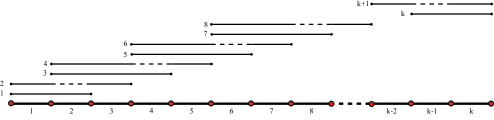
Figure 2: Integrality Gap for PLC

We now show that the integrality gap of the canonical LP for PLC is bounded by $2$. We describe a simple primal-dual algorithm that constructs a feasible line cover solution and a feasible dual solution, and the cost of the former is at most twice the value of the dual solution.

The algorithm maintains a set of segments $Q$. Call an edge $e$ unsatisfied if no segment in $Q$ covers $e$. Let $U$ be the set of unsatisfied edges. Initially $Q$ is the empty set and $U=E$. We grow duals $y_{e}$ on certain edges, as specified below. We let $E_{+}$ denote the edges with positive $y_{e}$; we call such edges, positive edges. Initially $E_{+}$ is empty. Call a segment $j$ tight if $\sum_{e\in j:j~{}covers~{}e}y_{e}=c_{j}$. We use the terminology an edge $e$ is larger than $f$, if $\mathrm{\pi}_{e}\geq\mathrm{\pi}_{f}$.

Primal-Dual Algorithm 1. While $U$ is not empty do • Breaking ties arbitrarily, pick the largest edge $e$ in $U$. • Increase $y_{e}$ till some segment becomes tight. Note that each such segment must contain $e$. Let $j_{l}(e)$ and $j_{r}(e)$ be the tight segments that have the smallest left-end-point and the largest right-end-point, respectively. Since $e$ is chosen to be the largest uncovered edge, any unsatisfied edge contained in the two segments $j_{l}(e)$ or $j_{r}(e)$ is also covered. We say $e$ is responsible for $j_{l}(e)$ and $j_{r}(e)$. Add $j_{l}(e),j_{r}(e)$ to $Q$. Add $e$ to $E_{+}$. Remove all the unsatisfied edges contained in either $j_{l}(e)$ or $j_{r}(e)$ from $U$. 2. Reverse Delete: Scan the segments $j$ in $Q$ in the reverse order in which they were added, and delete $j$ if its deletion doesn’t lead to uncovered edges.

It is clear that the final set $Q$ is feasible. It is also clear that $y$ forms a feasible dual. The factor $2$-approximation follows from the following lemma by a standard relaxed complementary slackness argument, and this finishes the proof of Theorem 3.

Lemma 5.

Any edge $e\in E_{+}$ is covered by at most two segments in $Q$.

Proof.

Suppose there is an edge $e\in E_{+}$ covered by three segments $j_{1},j_{2}$ and $j_{3}$. Observe that one of the segments, say $j_{2}$, must be completely contained in $j_{1}\cup j_{3}$. Since $j_{2}$ is not deleted from $Q$, there must be an edge $f\in j_{2}$ such that $j_{2}$ is the only segment in $Q$ covering $f$. Since $j_{1}$ and $j_{3}$ don’t cover $f$, but one of them, say $j_{1}$ contains it, this implies $\mathrm{\pi}_{f}>\sup_{j_{1}}\geq\mathrm{\pi}_{e}$. That is, $f$ is larger than $e$.

If $f$ is the edge responsible for $j_{2}$, then since $j_{2}$ contains $e$, $e$ wouldn’t be in $E_{+}$. Since $f$ is larger than $e$, there must be a segment $j$ in $Q$ added before $j_{2}$ that covers $f$. In the reverse delete order, $j_{2}$ is processed before $j$. This contradicts that $j_{2}$ is the only segment in $Q$ covering $f$. ∎

Lemma 6.

$\sum_{j\in Q}c_{j}\leq 2\sum_{e\in E}y_{e}$.

Proof.

Since each $s\in Q$ satisfies $\sum_{e\in j:j~{}covers~{}e}y_{e}=c_{j}$, we get

$$\sum_{j\in Q}c_{j}=\sum_{j\in Q}\sum_{e\in j:j~{}covers~{}e}y_{e}=\sum_{e\in E}y_{e}\cdot|\{j\in Q:j~{}covers~{}e\}|\leq 2\sum_{e\in E}y_{e}$$

∎

3.2 An Exact Algorithm for PLC

We first describe the sketch of the algorithm; the full proof starts from Section 3.2.1. A segment $j$ covers only a subset of edges it contains. We call a contiguous interval of edges covered by $j$, a valley of $j$. The uncovered edges form mountains. Thus a segment can be thought of as forming a series of valleys and mountains.

Given a solution $S\subseteq\mathcal{S}$ to the PLC (or even a PTC) instance, we say that segment $j\in S$ is needed for edge $e$ if $j$ is the unique segment in $S$ that covers $e$. We let $E_{S,j}$ be the set of edges that need segment $j$. We say a solution is valley-minimal if it satisfies the following two properties: (a) If a segment $j$ is needed for edge $e$ that lies in the valley $v$ of $j$, then no higher supply segment of $S$ intersects this valley $v$, and (b) every segment $j$ is needed for its last and first edges. We show that an optimum solution can be assumed to be valley-minimal, and thus it suffices to find the minimum cost valley-minimal solution.

The crucial observation follows from properties (a) and (b) above. The valley-minimality of solution $S$ implies that there is a unique segment $j\in S$ that covers the first edge of the line. At a very high level, we may now use $j$ to decompose the given instance into a set of smaller instances. For this we first observe that each of the remaining segments in $S\setminus\{j\}$ is either fully contained in the strict interior of segment $j$, or it is disjoint from $j$, and lies to the right of it. The set of all segments that are disjoint from $j$ form a feasible solution for the smaller PLC instance induced by the portion of the original line instance to the right of $j$. On the other hand, we show how to reduce the problem of finding an optimal solution for the part of the line contained in $j$ to a single shortest-path computation in an auxiliary digraph. Each of the arcs in this digraph once again corresponds to a smaller sub-instance of the original PLC instance, and its cost is that of its optimal solution. The algorithm follows by dynamic programming.

3.2.1 Valley-Minimal Solutions

As mentioned above, it helps to think of supplies and demands as heights. In the case of PLC, the demands of the edges in $E$ form a terrain, and each segment $j\in\mathcal{S}$ corresponds to a straight line at height $\mathrm{s}_{j}$. Segment $j$ then covers edge $e$ if $e$ lies in the segment’s shadow, that is, the height of $e$ is smaller than the height of the segment.

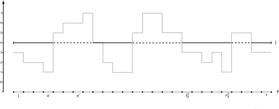
Figure 3: The figure shows a segment $j$, and the terrain induced by the edges of $E$ that it contains. The terrain partitions $j$ into valleys and mountains. Valleys are indicated by solid parts of $j$, and mountains are shown as dashed lines.

Figure 3 illustrates this with path $P$ and its edges. The light gray terrain indicates the demands of the edges. The segment $j$ shown in the picture covers the edges in $[l,r]$ that lie in its shadow; e.g., $j$ covers edge $e$ but not $e^{\prime}$. The terrain partitions $j$ naturally into valleys – contiguous sub-intervals of $[l,r]$ that are in the shadow of $j$, and mountains – those sub-intervals that are contained in $[l,r]$ and consist entirely of edges that are not covered by $j$. The parts of $j$ that correspond to mountains are indicated by dashed lines, and valleys are depicted by solid lines. In the following, we let $[l^{j}_{k},r^{j}_{k}]$ be the interval corresponding to the $k$th valley of $j$.

In the following, we will assume that the set of segments $\mathcal{S}$ in the given PLC/PTC instance is segment-complete; i.e., if $\mathcal{S}$ contains the segment $j$ then it also contains all proper sub-segments. For example, if a PLC instance contains segment $j$ corresponding to interval $[l^{j},r^{j}]$, then it also contains segments corresponding to intervals $[l,r]$ for all $l^{j}\leq l\leq r\leq r^{j}$. This assumption is w.l.o.g. as we can always add a dummy sub-segment $j^{\prime}$ for any such interval $[l,r]$ with the same supply and cost as $j$. Any minimal solution clearly uses at most one of $j$ and $j^{\prime}$, and if $j^{\prime}$ is used, then replacing it with $j$ does not affect feasibility.

Let $S\subset\mathcal{S}$ be an inclusion-wise minimal solution for the given instance, and let $j\in S$ be any one of its segments. We say that $j$ is needed for edge $e\in E$ if $j$ covers $e$, and if there is no other segment in $S$ that covers $e$; let $E_{S,j}$ be the set of edges that need $j$, and hence $E_{S,j}\neq\varnothing$ for all $j\in S$. Thus, if $j$ is needed for $e$, then $e$ is in one of $j$’s valleys; we let $\mathrm{val}^{j}_{e}$ be that valley.

A solution $S\subseteq\mathcal{S}$ is valley-minimal if

• for all $j\in S$ and for all $e\in E_{S,j}$, no segment of higher supply in $S$ covers any of the edges in $\mathrm{val}^{j}_{e}$, and

• each segment is needed for its first and last edge.

We obtain the following observation.

Lemma 7.

Given a feasible instance of PLC/PTC, there exists an optimum feasible solution that is valley-minimal.

Proof.

First, it is not too hard to see that we can always obtain an optimal solution that satisfies [M2]. If $S$ is an optimum solution with a segment $j$, and $j$ is not needed for its first or last edge $e$, then we may clearly replace $j$ by the sub-segment $j-e$. This does not increase the solutions cost, using the segment-completeness.

Assume, for the sake of contradiction that $S$ violates [M1]. For a solution $S\subseteq\mathcal{S}$, say that $(j,j^{\prime},e)$ is a violating triple if $j,j^{\prime}\in S$, $j^{\prime}$ has higher supply than $j$, $j$ is needed for $e$, and $j^{\prime}$ covers some edge in $\mathrm{val}^{j}_{e}$. Choose a solution $S$ with the smallest number of violating triples and let $(j,j^{\prime},e)$ be one such triple. Since $j$ is needed for $e$, edge $e$ is not contained in $j^{\prime}$, and hence $j^{\prime}$ is either fully contained in the interval $(e,n]$ or fully contained in the interval $[1,e)$. Using the segment-completeness assumption, we may replace $j^{\prime}$ by the sub-segment $j^{\prime\prime}$ obtained by removing the prefix consisting of edges in $\mathrm{val}^{j}_{e}$; remove $j^{\prime\prime}$ if it is empty. The resulting set of segments has cost at most that of $S$, and the number of violating triples is smaller; a contradiction. ∎

In the next subsection, we show how we can compute the minimum cost valley-minimal solution for PLC instances in polynomial time using dynamic programming.

3.2.2 Computing valley-minimal solutions

Given $1\leq l\leq r\leq n$, we obtain the sub-instance induced by interval $[l,r]$ by restricting the line $[1,n]$ to this interval, and by keeping only segments that are fully contained in $[l,r]$. Observe that the valley-completeness assumption implies that any such sub-instance is feasible. We begin by making a crucial observation that will allow us to decompose a given PLC instance into smaller instances. Let $S$ be a valley-minimal solution for the sub-instance induced by $[l,r]$, and note that [M2] implies that $S$ contains a unique segment $j$ that covers the first edge $(l,l+1)$. Suppose that $E_{S,j}=\{e_{1},\ldots,e_{k}\}$ is the set of edges within $[l,r]$ that need segment $j$. Abusing notation slightly, we let $\mathrm{val}^{j}_{i}=[l^{j}_{i},r^{j}_{i}]$ be the valley of $j$ around edge $e_{i}$; thus we clearly have

$$E_{S,j}\subseteq\mathrm{val}^{j}_{1}\cup\ldots\cup\mathrm{val}^{j}_{k}.$$ (16)

Note that segment $j$ may have valleys that entirely consist of edges that do not need $j$; accordingly, such valleys are not part of the list on the right-hand side of (16). Using property [M2], however, we may assume that $\mathrm{val}^{j}_{1}$ and $\mathrm{val}^{j}_{k}$ are the first and last valley, respectively, of segment $j$. We obtain the following observation, where we let $l^{j}_{k+1}=r+1$.

Observation 1.

We may assume, for all $1\leq i\leq k$, if $j^{\prime}\in S$ contains $e\in(r^{j}_{i},l^{j}_{i+1})$, then $j^{\prime}$ is fully contained in $(r^{j}_{i},l^{j}_{i+1})$.

Proof.

Consider first a segment $j^{\prime}\in S$ with supply bigger than $s_{j}$. In this case [M1] implies that $j^{\prime}$ must have an empty intersection with the valleys $\mathrm{val}^{j}_{1},\ldots,\mathrm{val}^{j}_{k}$, and the observation follows.

On the other hand if segment $j^{\prime}$ has supply at most $s_{j}$, then since $j^{\prime}$ must be needed for some edge $e$, $j$ must not contain $e$ implying $j^{\prime}$ must have its right end-point in $(r^{j}_{k},r]$. Replacing $j^{\prime}$ by its intersection with $(r^{j}_{k},r]$ completes the observation. ∎

We now let $\mathtt{OPT}_{l,r}$ be a minimum cost valley-minimal feasible solution for the sub-instance induced by interval $[l,r]$, and we let $\mathtt{opt}_{l,r}$ be its cost. Clearly, $\mathtt{OPT}_{n,n}$ consists of the minimum cost segment in $\mathcal{S}$ that covers edge $n$, and $\mathtt{OPT}_{1,n}$ is the optimum solution we want to obtain. Suppose that we know $\mathtt{OPT}_{l^{\prime},r^{\prime}}$ for all $l<l^{\prime}\leq r^{\prime}<r$. The high level idea is the following. The algorithm guesses the first segment $j$ in $\mathtt{OPT}_{l,r}$. Suppose that $r^{\prime}\leq r$ is the rightmost edge covered by $j$. Observation 1 allows us to partition the remaining segments in $\mathtt{OPT}_{l,r}$ into two parts:

Part 1

Segments that contain edges in $(r^{\prime},r]$. None of these segments can contain any of the edges in $[l,r^{\prime}]$ by the observation.

Part 2

Segments that contain edges in $[l,r^{\prime}]$. Once again, the observation implies that such segments must be fully contained in $(l,r^{\prime})$.

The first part’s solution is obtained since it is a smaller subproblem, the second part is obtained via a shortest-path computation. We now elaborate and give the complete algorithm.

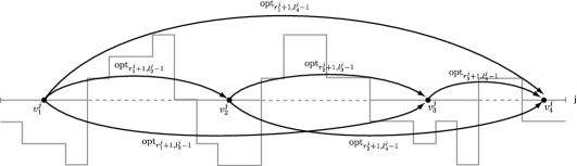
Figure 4: The part of digraph $G_{l}$ corresponding to segment $j\in\mathcal{S}_{l}$.

Let $\mathcal{S}_{l}$ be the segments in $\mathcal{S}$ with leftmost endpoint $l$. We construct a digraph $G_{\ell}$ as follows. Consider a segment $j\in\mathcal{S}_{l}$, and let

$$[l^{j}_{1},r^{j}_{1}],\ldots,[l^{j}_{k},r^{j}_{k}]$$

be the set of its valleys. We add a node $v^{j}_{q}$ for each valley $1\leq q\leq k$ of $j$ to $G_{\ell}$. We also add an arc $(v^{j}_{q},v^{j}_{q^{\prime}})$ for all $1\leq q<q^{\prime}\leq k$. A shortest path corresponding to the solution $\mathtt{OPT}_{l,r}$ will use arc $(v^{j}_{q},v^{j}_{q^{\prime}})$ if

• $j$ is the leftmost segment in $\mathtt{OPT}_{l,r}$, and

• $\mathrm{val}^{j}_{q}$ and $\mathrm{val}^{j}_{q^{\prime}}$ are two consecutive valleys of $j$ that contain edges that need $j$.

Observation 1 then states that $\mathtt{OPT}_{l,r}$ uses segments that are entirely contained in $(r^{j}_{q},l^{j}_{q^{\prime}})$ to cover $(r^{j}_{q},l^{j}_{q^{\prime}})$. An optimum set of such segments is given by $\mathtt{OPT}_{r^{j}_{q}+1,l^{j}_{q^{\prime}}-1}$, and we therefore give arc $(v^{j}_{q},v^{j}_{q^{\prime}})$ cost $\mathtt{opt}_{r^{j}_{q}+1,l^{j}_{q^{\prime}}-1}$. Figure 4 shows the part of $G_{\ell}$ for the segment $s$ from Figure 3.

We add a source node $s_{l}$ and arcs $(s_{l},v^{j}_{1})$ of cost $c_{j}$ for each of the segments $j\in\mathcal{S}_{l}$. A shortest path uses such an arc if $j$ is the unique segment starting at $l$ in the corresponding optimum solution. We also add a sink node $t_{r}$ and add an arc $(v^{j}_{k},t_{r})$ for all $j\in\mathcal{S}_{l}$ of cost $\mathtt{opt}_{r^{j}_{k}+1,r}$ indicating the optimum PLC for the sub-interval $[r^{j}_{k}+1,r]$. Note that if $r^{j}_{k}=r$, then this arc is a loop of cost $0$ and can be discarded.

It follows from the above construction that $\mathtt{opt}_{l,r}$ is equal to the cost of a shortest $s_{l},t_{r}$-path in $G_{l}$. Each of the shortest-path computations can clearly be done in polynomial time, and hence $\mathtt{opt}_{l,r}$ can be obtained via dynamic programming, in polynomial time. This yields the following restatement of Theorem 5.

Theorem 10.

The cost $\mathtt{opt}_{1,n}$ of an optimum solution for a given PLC instance can be computed in polynomial time.

4 Priority tree cover

We first give a proof of Theorem 6, and show that rooted PTC is APX-hard, even if all segments have unit cost. Subsequently, we present a $2$-approximation algorithm for the problem, by reducing it to an auxiliary instance of the tree augmentation problem. Then, we prove Theorem 4, and show that the integrality gap of the canonical LP formulation of unweighted PTC is bounded by $6$. Finally, we prove the connection between PTC and the rectangle cover problem.

4.1 APX-hardness

We prove APX-hardness of PTC via a reduction from the minimum vertex cover problem in bounded degree graphs. The latter problem is known to be APX-hard [3]. Given a bounded degree graph $G(V,E)$, with $n$ vertices and $m=O(n)$ edges, let the edges be arbitrarily numbered $\{1,2,\ldots,m\}$.

The tree in our instance has a broom structure: it has a handle which is a path of $m$ edges $(e_{1},\ldots,e_{m})$ given by vertices $\{x_{0},x_{1},\ldots,x_{m}\}$, and it has $n$ bristles where each bristle corresponds to a particular vertex $v\in V$ and is a path of length $deg(v)$. The edge $e_{i}$ in the handle for $1\leq i\leq m$, corresponds to the edge numbered $i$ in the graph $G$. The bristle corresponding to vertex $v$ is a path $(f^{v}_{1},f^{v}_{2},\ldots,f^{v}_{deg(v)})$ given by the vertices $\{x_{m},y^{v}_{1},y^{v}_{2},\ldots,y^{v}_{deg(v)}\}$. The root of the tree is $x_{0}$, the end point of the handle. Thus the tree has $m+\sum_{v}deg(v)=3m$ edges.

We now describe the priority demands of these tree edges. The demand of edge $e_{i}$ is $i$. Consider the edges in $G$ incident on $v$ in the decreasing order of their numbers. Suppose they are $(i_{1}>i_{2}>\cdots>i_{deg(v)})$. The demands of the edge $f^{v}_{j}$ is $i_{j}$. Thus, for a particular bristle corresponding to a vertex $v$, the demands decrease as we go from $f^{v}_{1}$ to $f^{v}_{deg(v)}$, and these demands correspond to the numbers of edges incident on $v$.

Now we describe the segments. All segments have unit cost. We have two kinds of segments: edge segments and vertex segments. For every edge $i=(v,w)$ in $E$, there are two edge segments $s^{i}_{v}$ and $s^{i}_{w}$. Segments $s^{i}_{v}$ contains all edges $e_{i}$ to $e_{m}$ and edges $f^{v}_{1}$ to $f^{v}_{j}$, where edge $i$ is the $j$th edge in the descending order of neighbors of $v$ in $G$. The supply of segment $s^{i}_{v}$ is $i$, and thus by construction, we see that $s^{i}_{v}$ only spans edge $e_{i}$ and $f^{v}_{j}$. That completes the description of edge segments. For every vertex $v$, there is a vertex segment $t_{v}$ that covers all the edges in the bristle corresponding to vertex $v$. That completes the description of the PTC instance. Look at figure 5 for an illustration of the reduction.

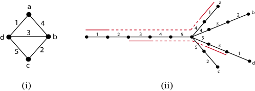
Figure 5: (i) shows an instance of the vertex cover problem, and (ii) is the corresponding PTC instance. The numbers on the edges are the priority demands corresponding to the edge numbers in the graph. Figure (ii) also shows two segments: $s^{1}_{a}$ and $s^{3}_{d}$, having supplies $1$ and $3$ respectively. Dashed line means that these segments do not have enough supply to cover the edges.

The following lemma along with the APX-hardness of the vertex cover problem in bounded degree graphs, and the fact that in the latter any vertex cover is of size $\Omega(n)$, leads to the APX-hardness of the PTC problem.

Lemma 8.

The optimum PTC of the above instance is $m+k$, where $k$ is the size of the optimum vertex cover of $G$.

Proof.

Firstly note that we may assume that in any optimal PTC, for any edge $i=(v,w)$, we will have exactly one of $s^{i}_{v}$ or $s^{i}_{w}$ in the solution. We need to have one since these are the only two segments that cover edge $e_{i}$ in the tree. Instead of picking both, we can remove one, say $s^{i}_{w}$, from the solution and pick the corresponding vertex segment $t_{w}$ instead, at no increase of cost. Therefore, there are exactly $m$ edge segments picked in any optimal PTC solution.

Now note that these $m$ edge segments uniquely correspond to an orientation of the edges in $G$; if for edge $i=(v,w)$, $s^{i}_{v}$ is chosen in the solution, the edge $(v,w)$ is oriented from $w$ to $v$. In this orientation, if there is a sink (a vertex with all edges incident to it) $v$, then note that all the edges in the bristle corresponding to $v$ have also been covered. Thus, the number of vertex segments required to cover the remaining edges of the tree, is precisely the number of non-sinks in this orientation. In particular, the optimal PTC corresponds to the orientation that minimizes the number of non-sinks.

The proof is complete by noting that non-sinks form a vertex cover; this is because each edge is oriented away from some non-sink, and is thus incident to it. Furthermore, given a vertex cover, there exists an orientation with precisely these vertices as non-sinks. Orient the edges towards the complement of the vertex cover (the independent set) - the complement is precisely the set of sinks, and thus the vertex cover is precisely the set of non-sinks. ∎

Proof of Theorem 6.

Suppose the degrees of $G$ are all $B$, a constant. Note that the vertex cover of this graph is at least $m/B=n/2$. The APX-hardness implies that it is NP-hard to distinguish between the case when the vertex cover is $c_{1}n$ or $c_{2}n$ where $c_{2}>c_{1}\geq 1/2$ are certain constants.

The above lemma therefore implies it is NP-hard to distinguish between the cases when the optimum of a PTC is $m+c_{1}n=(c_{1}+B/2)n$ and when the optimum is $m+c_{2}n=(c_{2}+B/2)n$. Since $B,c_{1},c_{2}$ are constants, we get the APX-hardness.

(For the interested reader: the APX-hardness of vertex cover of bounded degree graphs by Berman and Karpinski [3] gives $B=4$, $c_{1}=78/152$ and $c_{2}=79/152$, showing it is NP-hard to approximate to a factor better than $1.002$.) ∎

4.2 An approximation algorithm for PTC

The crucial idea is the following. Given an optimum solution $S^{*}\subseteq\mathcal{S}$, we can partition the edge-set $E$ of $T$ into disjoint sets $E_{1},\ldots,E_{p}$, and partition two copies of $S^{*}$ into $S_{1},\ldots,S_{p}$, such that $E_{i}$ is a path in $T$ for each $i$, and $S_{i}$ is a priority line cover for the path $E_{i}$. Once again, we assume without loss of generality that the instance is segment-complete.

In particular, we prove the following lemma. Let $\hat{E}_{S^{*},j}$ be the set of edges $e$ such that $j$ is the segment with the highest supply, among all segments in $S^{*}$ that cover $e$. Note that the union of all $\hat{E}_{S^{*},j}$, over all $j\in S^{*}$, partitions $E$. Also note that for each edge $e$, there is a unique segment $j$ such that $e\in\hat{E}_{S^{*},j}$. If there were two, we could replace one of the segments by a sub-segment and still stay feasible. We call the segment $j$ responsible for $e$.

Lemma 9.

Given an optimal solution $S^{*}\subseteq\mathcal{S}$ to a PTC instance with tree $T=(V,E)$, there is a partition

$$E_{1}\cup\ldots\cup E_{p}=E,$$

where each $E_{i}$ is the edge set of a path in $T$ such that for all $j\in S^{*}$, $\hat{E}_{S^{*},j}\cap E_{i}\neq\varnothing$ for at most two $i\in\{1,\ldots,p\}$.

Using this, we describe the $2$-approximation algorithm which proves Theorem 7.

Proof of Theorem 7.

For any two vertices $t$ (top) and $b$ (bottom) of the tree $T$, such that $t$ is an ancestor of $b$, let $P_{tb}$ be the unique path from $b$ to $t$. Note that $P_{tb}$, together with the restrictions of the segments in $\mathcal{S}$to $P_{tb}$, defines an instance of PLC. Therefore, for each pair $t$ and $b$, we can compute the optimal solution to the corresponding PLC instance; let the cost of this solution be $c^{\prime}_{tb}$. Create an instance of the 0,1-tree cover problem with $T$ and segments $\mathcal{S}^{\prime}:=\{(t,b):t\mbox{ is an ancestor of }b\}$ with costs $c^{\prime}_{tb}$. Solve the 0,1-tree cover instance exactly (recall we are in the rooted version) and for the segments $(t,b)$ in $\mathcal{S}^{\prime}$ returned, return the solution of the corresponding PLC instance of cost $c^{\prime}_{tb}$. We now use Lemma 9 to obtain a solution to the 0,1-tree cover problem $(T,\mathcal{S}^{\prime})$ of cost at most $2$ times the cost of $S^{*}$. This will prove the theorem.

For each $E_{i}$, let $t_{i}$ and $b_{i}$ be the end points of $E_{i}$ with $t_{i}$ being the ancestor of $b_{i}$. Since $E_{i}$’s partition the edges, the segments $(t_{i},b_{i}):i=1,\ldots,p$ is a feasible 0,1-tree cover for $(T,\mathcal{S}^{\prime})$. Define $S_{i}:=\{j\in S^{*}:e\in E_{i}\cap\hat{E}_{S^{*},j}\}$ to be the set of segments responsible for the edges in $E_{i}$. By definition, $S_{i}$ is a PLC for $E_{i}$. Thus, the cost of the segments in $S_{i}$ is at least $c^{\prime}_{t_{i}b_{i}}$. Furthermore, Lemma 9 implies that the total cost of the segments in $S_{i}$ is at most twice the cost of segments in $S^{*}$. Therefore, the cost of the feasible solution to the cover problem in $(T,\mathcal{S}^{\prime})$ is at most twice the cost of segments in $S^{*}$.

∎

Proof of Lemma 9.

We give an algorithm to compute the decomposition. Let $e$ be any of the edges incident to the root of $T$, and let $j_{1}\in S^{*}$ be the highest-supply segment covering $e$. We then let $E_{1}$ be the edges of the path in $T$ corresponding to $j_{1}$. Removing $E_{1}$ from $T$ yields sub-trees $T_{1},\ldots,T_{q}$. For each tree $T_{i}$ we repeat the above steps, and let

$$E_{1},\ldots,E_{p}$$ (17)

be the final partition; let $j_{i}\in S^{*}$ be the segment corresponding to edge-set $E_{i}$. Note that for $q<q^{\prime}$, $\hat{E}_{S^{*},j_{q}}\cap E_{q^{\prime}}$ is empty. This is because $E_{q^{\prime}}$ is a subset of edges which are not in $j_{q^{\prime}-1},\ldots,j_{1}$.

Consider a segment $j\in S$, and let $1\leq i\leq p$ be smallest such that $\hat{E}_{S^{*},j}\cap E_{i}\neq\varnothing$, and assume that $\hat{E}_{S^{*},j}\cap E_{q}\neq\varnothing$ for some $i<q\leq p$; choose $q$ smallest with this property. We claim that $j_{q}=j$, and hence for all $q<q^{\prime}\leq p$ we have $\hat{E}_{S^{*},j}\cap E_{q^{\prime}}=\emptyset$. Thus, $\hat{E}_{S^{*},j}$ has non-empty intersection only with $E_{i}$ and $E_{q}$.

Let $e\in E_{S^{*},j}\cap E_{i}$, and let $f\in E_{S^{*},j}\cap E_{q}$ be two edges in different parts of the partition such that $j$ is responsible for both. As both $e$ and $f$ are edges on $j$, and since $i<q$, it follows that $f$ is a descendant of $e$ in tree $T$. Let $g$ be the topmost edge of $E_{q}$; clearly, $g$ is on the $e,f$-path in $T$. By the decomposition algorithm, segment $j_{q}$ is the highest-supply segment covering edge $g$. As $j$ contains $g$, this means that the supply of $j_{q}$ is at least that of $j$. Finally, since $f$ is on $j_{q}$, $j_{q}$ covers $f$ as well. But this means that $j_{q}=j$ as $j$ is responsible for $f$. ∎

4.3 Canonical LP relaxation of PTC: Integrality Gap

In this section, we prove Theorem 4, by showing that the canonical LP relaxation of unweighted PTC is at most $6$. Recall the PTC LP.

$$\min~{}~{}\left\{\sum_{s\in\mathcal{S}}c_{s}x_{s}:~{}~{}\forall e\in E:\sum_{s:s~{}covers~{}e}x_{s}\geq 1;~{}~{}x_{s}\geq 0,\forall s\in\mathcal{S}\right\}$$ (18)

Proof of Theorem 4.

The idea of the proof is the following: as in the factor $2$-approximation for PTC, we decompose the edge set of the tree into disjoint sets $E_{1},\cdots,E_{p}$, such that each $E_{i}$ induces a path. We will abuse notation and refer to the $E_{i}$’s as paths. Furthermore, we take any feasible solution $x$ of (18) and obtain $p$ fractional solutions $x^{(1)},\ldots,x^{(p)}$ such that $x^{(i)}$ is a feasible fractional solution to (Primal) for the PLC instance on the path $E_{i}$. We will guarantee that

$$\sum_{i=1}^{p}\sum_{j\in\mathcal{S}}x^{(i)}_{j}\leq 3\sum_{j\in\mathcal{S}}x_{j}.$$

The theorem then follows from Theorem 3.

The figure shows a fragment $E_{i}$, its parent $E_{r}$, and two children $E_{s}$ and $E_{t}$. The segments $j_{1},j_{2}$, and $j_{3}$ are local for $E_{i}$, and segment $j_{4}$ is global. In particular, $j_{4}$ is an $i,t$-global segment.

(7cm,8cm)[fr]

Unlike in the argument used in the previous section where the decomposition into paths depended on $S^{*}$, the decomposition into disjoint paths that we use here is universal. Each path $E_{i}$ will end at a unique leaf, and $p$ in (17) will now be the number of leaves of $T$. Let $E_{1}$ be any path from the root to a leaf. Delete $E_{1}$ from the tree to get a series of sub-trees. Recursively, obtain $E_{2}$ to $E_{p}$. We call a path $E_{i}$ a child of $E_{q}$, if the starting point of $E_{i}$ lies on $E_{q}$.

Let $x$ be any feasible fractional solution of (18) and let $S^{*}$ be the support of $x$, that is, $S^{*}=\{j\,:\,x_{j}>0\}$. Fix a path $E_{i}$ and say that a segment $j\in S^{*}$ intersects $E_{i}$ if $j$ covers an edge in $E_{i}$ A segment $j$ that intersects $E_{i}$ is called local for $E_{i}$ if either the first or the last edge covered by $j$ lies in $E_{i}$. A segment $j$ that intersects $E_{i}$ is called global for $E_{i}$, otherwise. Figure 4.3 illustrates this.

Let $j$ be a global segment for $E_{i}$, and let $e$ be the first edge contained in $j$ after $E_{i}$. If $e\in E_{q}$, we call $s$ an $iq$-global segment. Observe that $E_{q}$ is a child of $E_{i}$. Thus an $iq$-global segment enters $E_{i}$ and exits via $E_{q}$. Note that $iq$-global segments, over all $q$ such that $E_{q}$ is a child of $E_{i}$, partition all global segments for $E_{i}$. Also note that an $iq$-global segment could also be a $i^{\prime}q^{\prime}$-global segment for some other $i^{\prime},q^{\prime}$.

Now we are ready to define the fractional solution $x^{(i)}$ that will be feasible for (Primal) for the PLC instance on $E_{i}$. Firstly for all segments $j$ that are local for $E_{i}$, let $x^{(i)}_{j}=x_{j}$. Next, we take care of segments that are global for $E_{i}$. For each child $E_{q}$ of $E_{i}$, order all the $iq$-global segments in non-increasing order of supply: $\{j_{1},\ldots,j_{r}\}$. Let $l$ be such that

$$x_{j_{1}}+\cdots+x_{j_{l}}\leq 1\mbox{ and }x_{j_{1}}+\cdots+x_{j_{l}}+x_{j_{l+1}}>1$$

If no such $l$ exists, then $l=r$. Define $x^{(i)}_{j_{k}}=x_{j_{k}}$ for $1\leq k\leq l$. If $l<r$, then let $x^{(i)}_{j_{l+1}}=1-\sum_{k=1}^{l}x^{(i)}_{j_{k}}$.

Claim 4.

$x^{(i)}$ is feasible for (Primal) for the PLC instance on $E_{i}$.

Proof.

Pick any edge $e\in E_{i}$. Look at all segments $j\in S^{*}$ that cover $e$. These segments are either local for $e$ or global for $e$. If $j$ is local, there is a corresponding segment in the support $x^{(i)}$ of the same value. Furthermore for any $q$,

$$\sum_{j:j\mbox{~{}is $iq$-global},j\mbox{ covers }e}x^{(i)}_{j}\geq\min\{1,\sum_{j:j\mbox{~{}is $iq$-global},j\mbox{ covers }e}x_{j}\}$$

In any case, $e$ is covered by $x^{(i)}$ at least to the extent it is covered by $x$, which implies $x^{(i)}$ is feasible. ∎

Lemma 10.

$\sum_{i=1}^{p}\sum_{j\in\mathcal{S}}x^{(i)}_{j}\leq 3\sum_{j\in\mathcal{S}}x_{j}$

Proof.

Each segment $j\in S^{*}$ is local for at most two paths $E_{i}$ and $E_{q}$. Thus the contribution to the LHS by local segments for some path $E_{i}$ is exactly $2\sum_{j\in\mathcal{S}}x_{j}$.

Furthermore, for every parent-child pair $E_{i}$ and $E_{q}$ that induces an $iq$-global segment for $E_{i}$, we increase the LHS by at most $1$. The number of such pairs is at most the number of leaves in $T$. The proof is complete by noting that $\sum_{j\in\mathcal{S}}x_{j}$ is at least the number of leaves in $T$. ∎

To complete the proof of the theorem, note that from Theorem 3 we know there exists for each $E_{i}$, a set of segments $S_{i}$ such that $|S_{i}|\leq 2\sum_{j\in\mathcal{S}}x^{(i)}_{j}$. The union of all such $S_{i}$ forms a valid PTC of cardinality at most $6\sum_{j\in\mathcal{S}}x_{j}$. ∎

4.4 Priority Tree Cover and Geometric Covering Problems

In this section, we show that the PTC problem is a special case of covering a set of points in $3$-dimension by axis-parallel rectangles (cuboids). In particular we prove Theorem 8. We go in two steps. We first define a problem, that we call $2$-Priority Line Cover and show that the PTC problem is a special case of $2$-PLC. Subsequently, we show $2$-PLC is a special case of $3$-dimensional rectangle cover. We start with a definition of $2$-PLC.

$2$-Priority Line Cover (2-PLC). The input is a line $T=(V,E)$, and a collection of segments $\mathcal{S}\subseteq V\times V$ with costs $c_{j}$ for each $j\in\mathcal{S}$. Furthermore, each segment $j$ has a priority supply vector in two dimensions, denoted as $(s^{1}_{j},s^{2}_{j})$, and each edge $e$ has a priority demand vector in two dimensions, denoted as $(\pi^{1}_{e},\pi^{2}_{e})$. A segment $j$ covers $e$ iff $j$ contains $e$ and $s^{i}_{j}\geq\pi^{i}_{e}$ for both $i=1,2$. The goal is to find the minimum cost collection of segments that cover every edge.

It is easy to see that PLC is a special case of $2$-PLC. Somewhat surprisingly, PTC is a special case of $2$-PLC as well.

Lemma 11.

Any instance of PTC can be encoded as an instance of 2-PLC with the same solution set.

Proof.

Given a rooted tree $T=(V,E)$, we perform two different depth first traversals to get two different orderings on the edges $E$. One such ordering will define the line of the 2-PLC instance, the other will define the first coordinates of the priority demand vectors of the edges.

In a depth first traversal of a tree, at every step we move from a vertex to one of its children, if any. Our two different traversals will be defined by two different choices of moving to a child-vertex. For every vertex $v$ of the tree, consider a total order $\sigma_{v}$ on its children. One such order that is convenient to keep in mind is the following; given a drawing of the tree, the total order of the children is from left to right. Let $\sigma^{R}_{v}$ be the opposite total order. The two depth first traversals are obtained by running with $\sigma_{v}$’s and $\sigma^{R}_{v}$’s, respectively. Figure 6 illustrates the two orders with the ordering $\sigma_{v}$ at every vertex $v$ being from left-to-right, and $\sigma^{R}_{v}$ being from right-to-left.

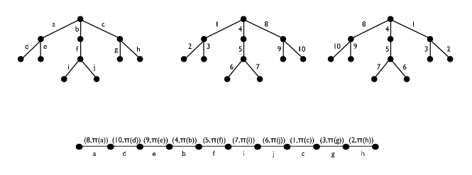
Figure 6: The left most tree is the original tree, the second and third are the two depth first traversals. The line below shows the line in the 2-PLC instance.

Let the two traversals return orderings $\mu$ and $\mu^{R}$ on the edges of the tree. The crucial observation is the following: for any vertex $v$, let $(v_{1},\ldots,v_{k})$ be the children in the $\sigma_{v}$ order; then $\mu(v,v_{1})<\mu(v,v_{2})<\cdots<\mu(v,v_{k})$, and thus, $\mu^{R}(v,v_{1})>\cdots>\mu^{R}(v,v_{k})$.

Now we are ready to describe the 2-PLC instance. The line is defined by the edges of the tree ordered w.r.t. $\mu$. That is, the order of the edges is $(e_{1},\ldots,e_{m})$ such that $\mu(e_{1})<\mu(e_{2})<\cdots<\mu(e_{m})$. The priority demand vector of an edge $e$ of the tree is $(\mu^{R}(e),\pi_{e})$. Consider a segment $j=(u,v)$ such that $u$ is a descendant of $v$ in the PTC instance. We identify two specific tree edges contained in $j$: the parent-edge $(u,u^{\prime})$ of $u$, and the edge $(v,v^{\prime})$ between node $v$ and its unique child $v^{\prime}$ that is on the $u,v$-path in $T$. By the depth-first property, we get $\mu(v,v^{\prime})\leq\mu(u,u^{\prime})$. The corresponding segment in the 2-PLC instance, also denoted as $j$, contains all the edges from $\mu(v,v^{\prime})$ to $\mu(u,u^{\prime})$. The priority supply vector of $j$ is $(\mu^{R}(u,u^{\prime}),s_{j})$.

Claim 5.

For any segment $j$, the set of edges covered by $j$ in the 2-PLC instance is precisely the set of edges covered in the PTC instance.

Proof.

Let $e$ be an edge covered by $j$ in the PTC instance. Since $e$ is contained in the path from $u$ to $v$ in the tree, by property of depth first traversals we get, $\mu(v,v^{\prime})\leq\mu(e)\leq\mu(u,u^{\prime})$ and $\mu^{R}(e)\leq\mu^{R}(u,u^{\prime})$. The first pair of inequalities implies $e$ lies in the segment $j$ in the 2-PLC instance, the second implies that $\pi^{1}_{e}\leq s^{1}_{j}$. Since $e$ is covered by $j$ in the PTC, we also get $\pi^{2}_{e}=\pi_{e}\leq s_{j}=s^{2}_{j}$. Thus, $e$ is covered by $j$ in the 2-PLC instance.

Let $e$ be an edge covered by $j$ in the 2-PLC instance. Since $e$ lies in $j$, we conclude $\mu(v,v^{\prime})\leq\mu(e)\leq\mu(u,u^{\prime})$. This implies either (a) $e$ lies on the path from $u$ to $v$ in the tree, or, (b) there is a node $w$ on the $u,v$-path in the tree, and a child $z$ of $w$ that is not on this path such that $e$ is contained in the subtree defined by edge $(w,z)$.

Note, that in case (b) the depth-first traversal for order $\sigma$ visits edge $(z,w)$ before edge $(u,u^{\prime})$. This implies that the second dfs traversal for order $\sigma^{R}$ visits $(z,w)$ after $(u,u^{\prime})$. Since $(z,w)$ is visited before $e$ in both traversals, we must therefore have $\mu^{R}(e)>\mu^{R}(u,u^{\prime})$, and this implies $s^{1}_{j}<\pi^{1}(e)$ which is impossible since $j$ covers $e$. Thus, case (b) is not possible, and $e$ lies on the path fro $u$ to $v$ on the tree. Furthermore, we have $s_{j}=s^{2}_{j}\geq\pi^{2}_{e}=\pi_{e}$, and so $j$ covers $e$ in the PTC instance as well. ∎

∎

Now we show that $2$-PLC is a special case of $3$-dimensional rectangle cover. This is not to hard to see. We assume the edges of the line are numbered $(1,2,\ldots,m)$. For edge $e$ numbered $e_{i}$, we associate a point in $3$ dimensions with coordinates $(i,\pi^{1}_{e},\pi^{2}_{e})$. For each segment $j=(a,b)$, we have a rectangle associated. In fact, these rectangles have are unbounded in the negative $y$ and $z$ coordinates. The other $4$ bounding half-spaces are $x\geq a$, $x\leq b$, $y\leq s^{1}(j)$ and $z\leq s^{2}(j)$. It is not too hard to see a rectangle corresponding to a segment $j$ contains a point corresponding to an edge $e$ iff $j$ covers $e$ in the 2-PLC instance. This completes the proof of Theorem 8.

5 Concluding Remarks

In this paper we studied column restricted covering integer programs. In particular, we studied the relationship between CCIPs and the underlying 0,1-CIPs. We conjecture that the approximability of a CCIP should be asymptotically within a constant factor of the integrality gap of the original 0,1-CIP. We couldn’t show this; however, if the integrality gap of a PCIP is shown to be within a constant of the integrality gap of the 0,1-CIP, then we will be done. At this point, we don’t even know how to prove that PCIPs of special 0,1-CIPS, those whose constraint matrices are totally unimodular, have constant integrality gap. Resolving the case of PTC is an important step in this direction, and hopefully in resolving our conjecture regarding CCIPs.

References

- [1] E. Balas. Facets of the knapsack polytope. Math. Programming, 8:146–164, 1975.
- [2] Amotz Bar-Noy, Reuven Bar-Yehuda, Ari Freund, Joseph Naor, and Baruch Schieber. A unified approach to approximating resource allocation and scheduling. J. ACM, 48(5):1069–1090, 2001.
- [3] P. Berman and M. Karpinski. On some tighter inapproximability results. In Proceedings, International Colloquium on Automata, Languages and Processing, pages 200–209, 1999.
- [4] R. D. Carr, L. K. Fleischer, V. J. Leung, and C. A. Phillips. Strengthening integrality gaps for capacitated network design and covering problems. In Proceedings, ACM-SIAM Symposium on Discrete Algorithms, pages 106–115, 2000.
- [5] M. Charikar, J. Naor, and B. Schieber. Resource optimization in qos multicast routing of real-time multimedia. IEEE/ACM Trans. Netw., 12(2):340–348, 2004.
- [6] C. Chekuri, A. Ene, and N. Korula. Unsplittable flow in paths and trees and column-restricted packing integer programs. In Proceedings, International Workshop on Approximation Algorithms for Combinatorial Optimization Problems, page (to appear), 2009.
- [7] C. Chekuri, M. Mydlarz, and F. B. Shepherd. Multicommodity demand flow in a tree and packing integer programs. ACM Trans. Alg., 3(3), 2007.
- [8] J. Cheriyan, H. Karloff, R. Khandekar, and J. Könemann. On the integrality ratio for tree augmentation. Operations Research Letters, 36(4):399–401, 2008.
- [9] J. Chuzhoy, A. Gupta, J. Naor, and A. Sinha. On the approximability of some network design problems. ACM Trans. Alg., 4(2), 2008.
- [10] G. Dobson. Worst-case analysis of greedy heuristics for integer programming with non-negative data. Math. Oper. Res., 7(4):515–531, 1982.
- [11] P. Hammer, E. Johnson, and U. Peled. Facets of regular 0-1 polytopes. Math. Programming, 8:179–206, 1975.
- [12] D. S. Hochbaum. Approximation algorithms for the set covering and vertex cover problems. SIAM Journal on Computing, 11(3):555–556, 1982.
- [13] S. G. Kolliopoulos. Approximating covering integer programs with multiplicity constraints. Discrete Appl. Math., 129(2-3):461–473, 2003.
- [14] S. G. Kolliopoulos and C. Stein. Approximation algorithms for single-source unsplittable flow. SIAM Journal on Computing, 31(3):919–946, 2001.
- [15] S. G. Kolliopoulos and C. Stein. Approximating disjoint-path problems using packing integer programs. Math. Programming, 99(1):63–87, 2004.
- [16] S. G. Kolliopoulos and N. E. Young. Approximation algorithms for covering/packing integer programs. J. Comput. System Sci., 71(4):495–505, 2005.
- [17] Nitish Korula. private communication, 2009.
- [18] S. Rajagopalan and V. V. Vazirani. Primal-dual RNC approximation algorithms for (multi)set (multi)cover and covering integer programs. In Proceedings, IEEE Symposium on Foundations of Computer Science, 1993.
- [19] A. Schrijver. Combinatorial optimization. Springer, New York, 2003.
- [20] A. Srinivasan. Improved approximation guarantees for packing and covering integer programs. SIAM Journal on Computing, 29(2):648–670, 1999.
- [21] A. Srinivasan. An extension of the lovász local lemma, and its applications to integer programming. SIAM Journal on Computing, 36(3):609–634, 2006.
- [22] L. Trevisan. Non-approximability results for optimization problems on bounded degree instances. In Proceedings, ACM Symposium on Theory of Computing, pages 453–461, 2001.
- [23] L. Wolsey. Facets for a linear inequality in 0-1 variables. Math. Programming, 8:168–175, 1975.