Coarse-graining schemes for stochastic lattice systems with short and long-range interactions

Abstract

We develop coarse-graining schemes for stochastic many-particle microscopic models with competing short- and long-range interactions on a $d$-dimensional lattice. We focus on the coarse-graining of equilibrium Gibbs states and using cluster expansions we analyze the corresponding renormalization group map. We quantify the approximation properties of the coarse-grained terms arising from different types of interactions and present a hierarchy of correction terms. We derive semi-analytical numerical schemes that are accompanied with a posteriori error estimates for coarse-grained lattice systems with short and long-range interactions.

1 Introduction

Many-particle microscopic systems with combined short and long-range interactions are ubiquitous in a variety of physical and biochemical systems, [35]. They exhibit rich mesoscopic and macroscopic morphologies due to competition of attractive and repulsive interaction potentials. For example, mesoscale pattern formation via self-assembly arises in heteroepitaxy, [33], other notable examples include polymeric systems, [14], and micromagnetic materials, [16]. Simulations of such systems rely on molecular methods such as kinetic Monte Carlo (kMC) or Molecular Dynamics (MD). However, the presence of long-range interactions severely limits the spatio-temporal scales that can be simulated by such direct computational methods.

On the other hand, an important class of computational tools used for accelerating microscopic molecular simulations is the method of coarse-graining. By lumping together degrees of freedom into coarse-grained variables interacting with new, effective potentials the complexity of the molecular system is reduced, thus yielding accelerated simulation methods capable of reaching mesoscopic length scales. Such methods have been developed for the study and simulation of crystal growth, surface processes and polymers, e.g., [19, 17, 25, 1, 8, 21], while there is an extensive literature in soft matter and complex fluids, e.g., [39, 28, 11, 12]. Existing approaches can give unprecedented speed-up to molecular simulations and can work well in certain parameter regimes, for instance, at high temperatures or low densities of the systems. On the other hand important macroscopic properties may not be captured properly in many parameter regimes, e.g., the melt structures of polymers, [25]; or the crystallization of complex fluids, [32]. Motivated in part by such observations we formulated and analyzed, from a numerical analysis and statistical mechanics perspective, coarse-grained variable selection and error quantification of coarse-grained approximations focusing on stochastic lattice systems with long-range interactions, [23, 22, 2, 21]. We have shown that the ensuing schemes, known as coarse-grained Monte Carlo (CGMC) methods, perform remarkably well even though traditional Monte Carlo methods experience a serious slow-down. In this paper we focus on lattice systems with both short and long-range interactions. Short-range interactions introduce strong correlations between coarse-grained variables and a radically different approach needs to be employed in order to carry out a systematic and accurate coarse-graining of such systems.

The coarse-graining of microscopic systems is essentially a problem in approximation theory and numerical analysis. However, the presence of stochastic fluctuations on one hand, and the extensive nature of the models (the presence of extensive quantities that scale as $\mathcal{O}(N)$ with the size of system $N$) on the other create a new set of challenges. Before we proceed with the main results of this paper we discuss all these issues in a general setting that applies to both on-lattice and off-lattice systems and present the mathematical and numerical framework of coarse-graining for equilibrium many-body systems.

We denote by $\sigma$ microscopic states of a many-particle system and by ${\mathcal{S}_{N}}$ the set of all microscopic states (i.e., the configuration space). The energy of a configuration is given by the Hamiltonian $H_{N}(\sigma)$ where $N$ denotes the size of the microscopic system. An example studied in this paper is the $d$-dimensional Ising-type model defined on a lattice with $N=n^{d}$ lattice points, and suitable boundary conditions, e.g., periodic. For both on-lattice or off-lattice particle systems the finite-volume equilibrium states of the system are given by the canonical Gibbs measure at the inverse temperature $\beta$, describing the most probable configurations

$$\mu_{N,\beta}(d\sigma)=\frac{1}{Z_{N}}e^{-\beta H_{N}(\sigma)}P_{N}(d\sigma)\,,$$ (1)

where the normalizing factor $Z_{N}=\int e^{-\beta H_{N}}P_{N}$, the partition function, ensures that (1) is a probability measure, and $P_{N}(d\sigma)$ denotes the prior distribution on ${\mathcal{S}_{N}}$. The prior distribution is typically a product measure (see for instance (11)) which describes non-interacting particle, or equivalently describes the system at infinite temperature $\beta=0$. At the $\beta=0$ limit the particle interactions included in $H_{N}$ are unimportant and thermal fluctuations, i.e., disorder, associated with the product structure of the prior, dominates the system. By contrast at the zero temperature limit, $\beta\to\infty$, interactions dominate and thermal fluctuations are unimportant; in this case (1) concentrates on the minimizers, also known as the “ground states”, of the Hamiltonian $H_{N}$ over all configurations $\sigma$. Finite temperatures, $0<\beta<\infty$, describe intermediate states to these two extreme regimes, including possibly phase transitions, i.e., regimes when as parameters, such as the temperature, change, the system exhibits an abrupt transition from a disordered to an ordered state and vice versa, or between different ordered phases.

The objective of (equilibrium) computational statistical mechanics is the simulation of averages over Gibbs states, (1) of observable quantities $f(\sigma)$

$${\mathbb{E}}_{\mu_{N\beta}}[f]\,=\,\int f(\sigma){\mu}_{N\beta}(d\sigma)\,.$$ (2)

Due to the exceedingly high dimension of the integration, even for moderate values of the system size $N$, e.g., $|{\mathcal{S}_{N}}|=2^{N}$ for the standard Ising model, such averaged observables are typically calculated by Markov Chain Monte Carlo (MCMC) methods, [27]. Nonetheless, mesoscale morphologies, e.g., traveling waves and patterns, are beyond the reach of conventional Monte Carlo methods. For this reason coarse-graining methods have been developed in order to speed up molecular simulations.

We briefly discuss the mathematical formulation and numerical analysis challenges arising in coarse-graining of an equilibrium system described by (1). We rewrite the microscopic configuration $\sigma$ in terms of coarse variables $\eta$ and corresponding fine variables $\xi$ so that $\sigma=(\eta,\xi)$. We denote the configuration space at the coarse level by $\bar{\mathcal{S}}_{M}$ and we denote by $\mathbf{F}$ the coarse-graining map $\mathbf{F}:{\mathcal{S}_{N}}\rightarrow\bar{\mathcal{S}}_{M}\,,\;\mathbf{F}\sigma=\eta\in\bar{\mathcal{S}}_{M}$. The coarse-grained system size is denoted by $M$, while the microscopic system size is $N=QM$, where we refer to $Q$ as the level of coarse-graining, and $Q=1$ corresponds to no coarse-graining.

At the coarse-grained level one is interested in observables $f(\eta)$ which depend only on the coarse variable $\eta$ and a coarse-grained statistical description of the equilibrium properties of the system should be given by a probability measure ${\bar{\mu}}_{M,\beta}(d\eta)$ on $\bar{\mathcal{S}}_{M}$ such that the average (the expected value) of such observable is same in the coarse-grained as well as fully resolved systems. This motivates the following definition.

Definition 1.

The exact coarse-grained Gibbs measure ${\bar{\mu}}_{M,\beta}$ is defined by

$${\bar{\mu}}_{M,\beta}(A)\,\equiv\,\mu_{N,\beta}(\mathbf{F}^{-1}(A))\,,$$ (3)

for any (measurable) set $A\subset\bar{\mathcal{S}}_{M}$ or, equivalently,

$$\int f(\eta)\,{\bar{\mu}}_{M,\beta}(d\eta)\,=\,\int f(\mathbf{F}(\sigma))\,\mu_{N,\beta}(d\sigma)\,.$$ (4)

for all (bounded) $f:\bar{\mathcal{S}}_{M}\to\mathbb{R}$.

Slightly abusing notation we will write ${\bar{\mu}}_{M,\beta}\,\equiv\,\mu_{N,\beta}\circ\mathbf{F}^{-1}$ in the sequel. In order to write the measure ${\bar{\mu}}_{M,\beta}$ in a more convenient form we first compute the exact coarse-graining of the prior distribution $P_{N}(d\sigma)$ on ${\mathcal{S}_{N}}$

$${\bar{P}}_{M}(d{\eta})=P_{N}\circ\mathbf{F}^{-1}\,.$$

The conditional prior probability $P_{N}(d\sigma{\,|\,}{\eta})$ of having a microscopic configuration $\sigma$ given a coarse configuration $\eta$ will play a crucial role in the sequel. Recall that for a function $g(\sigma)$ the conditional expectation is given by

$${\mathbb{E}}[g{\,|\,}{\eta}]\, = \,\int g(\sigma)\,P_{N}(d\sigma{\,|\,}{\eta})\,.$$ (5)

We now write the coarse-grained Gibbs measure ${\bar{\mu}}_{M,\beta}$ using a coarse-grained Hamiltonian $\bar{H}_{M}(\eta)$.

Definition 2.

The exact coarse-grained Hamiltonian $\bar{H}_{M}(\eta)$ is given by

$$e^{-\beta\bar{H}_{M}(\eta)} \,=\, {\mathbb{E}}[e^{-\beta H_{N}}{\,|\,}{\eta}]\,.$$ (6)

This procedure is known as a renormalization group map, [18, 15]. Note that the partition functions for $H_{N}$ and $\bar{H}_{M}$ coincide since

$$Z_{N}=\int e^{-\beta H_{N}}P_{N}(d\sigma)=\int\int e^{-\beta H_{N}}P_{N}(d\sigma{\,|\,}\eta){\bar{P}}_{M}(d\eta)=\int e^{-\beta\bar{H}_{M}}{\bar{P}}_{M}(d\eta)\equiv{\bar{Z}}_{M}\,.$$

Hence for any function $f(\eta)$ we have

$$\int f(\eta)\mu_{N,\beta}(d\sigma)\, = \,\int f(\eta)\frac{1}{Z_{N}}e^{-\beta H_{N}}P_{N}(d\sigma)\,=\,\int f(\eta)\frac{1}{Z_{N}}\int e^{-\beta H_{N}}P_{N}(d\sigma{\,|\,}\eta){\bar{P}}_{M}(d\eta)$$

$$= \,\int f(\eta)\frac{1}{{\bar{Z}}_{M}}e^{-\beta\bar{H}_{M}({\eta})}{\bar{P}}_{M}(d{\eta})\,,$$

and thus the coarse-grained measure ${\bar{\mu}}_{M,\beta}(d{\eta})$ in (3) is given by

$${\bar{\mu}}_{M,\beta}(d{\eta})=\frac{1}{{\bar{Z}}_{M}}e^{-\beta\bar{H}_{M}({\eta})}{\bar{P}}_{M}(d{\eta})\,.$$ (7)

Although typically ${\bar{P}}_{M}(d{\eta})$ is easy to calculate, see e.g., (12), the exact computation of the coarse-grained Hamiltonian $\bar{H}_{M}(\eta)$ given by (7) is, in general, an impossible task even for moderately small values of $N$.

In this paper we restrict our attention to lattice systems, and our main result is the development of a general strategy to construct explicit numerical approximations of the exact coarse-grained Hamiltonian $\bar{H}_{M}(\eta)$ in the physically important case of combined and competing short and long range interactions. Essentially we construct an approximate coarse-grained energy landscape for the original complex microscopic lattice system in Section 2. We show that there is an expansion of $\bar{H}_{M}(\eta)$ into a convergent series

$$\bar{H}_{M}(\eta)=\bar{H}_{M}^{(0)}(\eta)+\bar{H}_{M}^{(1)}(\eta)+\bar{H}_{M}^{(2)}(\eta)+\mbox{error}$$ (8)

by constructing a suitable first approximation $\bar{H}_{M}^{(0)}(\eta)$ and identifying small parameters to control the higher-order terms in the expansion. Truncations including a first few terms in (8) correspond to coarse-graining schemes of increasing accuracy. In order to obtain this expansion we rewrite (6) as

$$\bar{H}_{M}(\eta)=\bar{H}_{M}^{(0)}(\eta)-\frac{1}{\beta}\log{\mathbb{E}}[e^{-\beta(H_{N}-\bar{H}_{M}^{(0)}(\eta))}{\,|\,}{\eta}]\,.$$ (9)

We need to show that the logarithm can be expanded into a convergent series, uniformly in $N$, yielding eventually an expression of the type (8). However, two interrelated difficulties emerge immediately: (a) the stochasticity of the system in the finite temperature case yields the nonlinear expression in (9) which in turn will need to be expanded into a series; (b) the extensive nature of the microscopic system, i.e., typically the Hamiltonian scales as $H_{N}=\mathcal{O}(N)$, does not allow the expansion of the logarithm and exponential functions into the Taylor series.

For these reasons, one of the principal mathematical tools we employ is the cluster expansion method, see [36] for an overview and references. As we shall see in the course of this paper cluster expansions will allow us to identify uncorrelated components in the expected value ${\mathbb{E}}[e^{-\beta(H_{N}-\bar{H}_{M}^{(0)}(\eta))}{\,|\,}{\eta}]$, which in turn will permit us to factorize it, and subsequently expand the logarithm in (9) in order to obtain the series (8). The coarse-graining of systems with purely long-range interactions was extensively studied using cluster expansions in [22, 2, 21]. Here we are broadly following and extending this approach. However, the presence of both short and long-range interactions presents new difficulties and requires new methods based on the ideas developed in [31, 3]. Short-range interactions induce sub-grid scale correlations between coarse variables, and need to be explicitly included in the initial approximation $\bar{H}_{M}^{(0)}(\eta)$. To account for these effects we introduce a multi-scale decomposition of the Gibbs state (1) into fine and coarse variables, which in turn allows us to describe, in a explicit manner, the communication between scales for both short and long-range interactions. Furthermore, the multi-scale decomposition of (1) can also allow us to reverse the procedure of coarse-graining in a mathematically systematic manner, i.e., reconstruct spatially localized “atomistic” properties, directly from coarse-grained simulations. We note that this issue arises extensively in the polymer science literature, [38, 29].

An important outcome of the cluster expansion analysis for the approximation of (8) is the semi-analytical splitting scheme for the coarse-graining of lattice systems with short and long-range interactions. Presumably similar strategies could be applied for off-lattice systems such as the coarse-graining of polymers. The schemes proposed here can be split, within a controllable approximation error, into a long and a short-range calculation, see (40). The long-range part, which is computationally expensive for conventional Monte Carlo methods, can be cheaply simulated using the analytical formula given in (15) in the spirit of our previous work [22]. In this case the saving comes from reducing the degrees of freedom by $Q=N/M$ and compressing the range of interactions. For the short-range interactions we use the semi-analytical formulas (50) which involve precomputing coarse-grained interactions with Monte Carlo simulation. However, the simulation is done for a single subdomain of three adjacent coarse cells. The error estimates in Theorem 5 also suggest an improved decomposition to short and long-range interactions. Indeed, they imply splitting and rearrangement of the overall combined short and long-range potential into a new short-range component that includes possible singularities originally in the long-range interaction, e.g., the non-smooth part in a Lennard-Jones potential, and a locally integrable (or smooth) long-range decaying component.

In contrast to the splitting approach developed here that allows us to analytically calculate the long range effective Hamiltonian (16) in (40) and in parallel carry out the semi-analytical step for (50), existing methods, e.g., ([14, 25]), employ semi-analytical computations involving both short, as well as costly long-range interactions. Thus, multi-body terms, which are believed to be important at lower temperatures, [14], have to be disregarded. A notable result of our error analysis is the quantification of the role of multi-body terms in coarse-graining schemes, and the relative ease to implement them using the aforementioned splitting schemes. In Section 4, we further quantify the regimes where such multi-body terms are necessary in the context of a specific example. In [2] the necessity to include multi-body terms in the effective coarse-grained Hamiltonian was first discussed in a numerical analysis context for systems with singular (at the origin) long-range interactions.

Cluster expansions such as (8) can also be used for constructing a posteriori error estimates for coarse-graining problems, based on the rather elementary observation that higher-order terms in (46) can be viewed as errors that depend only on the coarse variables $\eta$. In [20] we already employed this type of estimates for stochastic lattice systems with long-range interactions in order to construct adaptive coarse-graining schemes. These tools operated as an “on-the-fly” coarsening/refinement method that recovers accurately phase-diagrams. The estimates allowed us to change adaptively the coarse-graining level within the coarse-graining hierarchy once suitably large or small errors were detected, and thus to speed up the calculations of phase diagrams. Adaptive simulations for molecular systems have been also recently proposed in [34], although they are not based on an a posteriori error analysis perspective. Finally, the cluster expansions necessary for the rigorous derivation and error estimates of the schemes developed here rely on the smallness of a suitable parameter introduced in Theorem 5, see (45). In Section 4, we construct an a posteriori bound for this quantity that can allow us to track the validity of the cluster expansion for a given resolution in the course of a simulation. This approach is, at an abstract level, similar to conditional a posteriori estimates proposed earlier in the numerical analysis of geometric partial differential equations, [13, 26].

Further challenges for systems with short and long-range interactions not discussed here include: error estimates for observables/quantities of interest, the development of coarse-grained dynamics from microscopics, phase transitions and estimation of physical parameters, such as critical temperatures. Work related to these directions for systems with long-range interactions have been carried out in [23], [5] and [4].

The paper is organized as follows. In Section 2 we present the microscopic Ising-type models with short and long-range interactions and introduce the coarse-graining maps and the resulting coarse-grained configuration spaces. In Section 3 we discuss our general strategy for the analysis of systems with short and long-range interactions and present our main results. In Section 4 we discuss semi-analytical coarse-graining schemes and their applications to specific examples. Section 5 is devoted to the construction of the cluster expansion and to the proof of convergence of our schemes.

Acknowledgments: The research of M.A.K. was supported by the National Science Foundation through the grants and NSF-DMS-0715125 and the CDI -Type II award NSF-CMMI-0835673, the U.S. Department of Energy through the grant DE-SC0002339, and the European Commission Marie-Curie grant FP6-517911. The research of P.P. was partially supported by the National Science Foundation under the grant NSF-DMS-0813893 and by the Office of Advanced Scientific Computing Research, U.S. Department of Energy under DE-SC0001340; the work was partly done at the Oak Ridge National Laboratory, which is managed by UT-Battelle, LLC under Contract No. DE-AC05-00OR22725. The research of L. R.-B. was partially supported by the grant NSF-DMS-06058. The research of D. K. T. was partially supported by the Marie-Curie grant PIEF-GA-2008-220385.

2 Microscopic lattice models and coarse-graining

We consider an Ising-type model on the $d$-dimensional square lattice ${\Lambda}_{N}:=\{x=(x_{1},\cdots,x_{d})\in\mathbb{Z}^{d}\,;\,0\leq x_{i}\leq n-1\}$ with $N=n^{d}$ lattice points. For simplicity we assume periodic boundary conditions throughout this paper although other boundary conditions can be accommodated. At each lattice site $x$ there is a spin $\sigma(x)$ taking values in $\Sigma=\{+1,-1\}$. A spin configuration $\sigma=\{\sigma(x)\}_{x\in{\Lambda}_{N}}$ on the lattice ${\Lambda}_{N}$ is an element of the configuration space ${\mathcal{S}_{N}}:=\Sigma^{{\Lambda}_{N}}$. For any subset $X\subset{\Lambda}_{N}$ we denote $\sigma_{X}=\{\sigma(x)\}_{x\in X}\in\Sigma^{X}$ the restriction of the spin configuration to $X$. Similarly, for a function $f:{\mathcal{S}_{N}}\to\mathbb{R}$ we denote $f_{X}$ the restriction of $f$ to $\Sigma^{X}$. The energy of a configuration $\sigma$ is given by the Hamiltonian

$$H_{N}(\sigma)=H_{N}^{s}(\sigma)+H_{N}^{l}(\sigma)\,,$$ (10)

which consists of a short-range part $H_{N}^{s}$ and a long range part $H_{N}^{l}$. For the short-range part we have

$$H_{N}^{s}(\sigma)\,=\,\sum_{X\subset{\Lambda}_{N}}U_{X}(\sigma)\,,$$

where the short-range potential $U=\{U_{X},\,X\subset\mathbb{Z}^{d}\}$, with $U_{X}:\Sigma^{X}\to\mathbb{R}$, is translation invariant (i.e., $U_{X+y}=U_{X}$ for all $X\subset\mathbb{Z}^{d}$ and all $y\in Z^{d}$) and has the finite range $S$ (i.e., $U_{X}=0$ whenever $\mbox{diam\,}(X)>S$). We define the norm $\|U\|\equiv\sum_{X\supset\{0\}{\,|\,}\mathrm{diam}(X)\leq S}\|U_{X}\|_{\infty}$ where the norm $\|\cdot\|_{\infty}$ is the standard sup-norm on the space of continuous functions. A typical case is the nearest-neighbor Ising model

$$H^{s}_{N}(\sigma)=K\sum_{\langle x,y\rangle}\sigma(x)\sigma(y)\,,$$

where by $\langle x,y\rangle$ we denote summation over the nearest neighbors. For the long-range part we assume the form

$$H_{N}^{l}(\sigma)\,=\,-\frac{1}{2}\sum_{x\in{\Lambda}_{N}}\sum_{y\neq x}J(x-y)\sigma(x)\sigma(y)\,,$$

where the two-body potential $J$ has the form

$$J(x-y)=\frac{1}{L^{d}}V\left(\frac{1}{L}|x-y|\right)\,,\;\;\;\\$$

for some $V\in C^{1}([0,\infty))$. The factor $1/L^{d}$ in (2) is a normalization which ensures that the strength of the potential $J$ is essentially independent of $L$, i.e., $\sum_{x\neq 0}|J(x)|\simeq\int|V(r)|dr$. For example, if we choose $V$ such that $V(r)=0$ for $r>1$ then a spin at the site $x$ interacts with its neighbors which are at most $L$ lattice points away from $x$ and in this case $L$ is the range of the interaction $J$. It is convenient to think of $L$ as a parameter in our model and more precise assumptions on the interactions will be specified later on.

The finite-volume equilibrium states of the system are given by the canonical Gibbs measure (1) and $P_{N}(d\sigma)$, the prior distribution on ${\mathcal{S}_{N}}$, is a product measure

$$P_{N}(d\sigma)=\prod_{x\in{\Lambda}_{N}}P_{x}(d\sigma(x))\,.$$ (11)

A typical choice is $P_{x}(\sigma(x)=+1)=\frac{1}{2}$ and $P_{x}(\sigma(x)=-1)=\frac{1}{2}$, i.e., independent Bernoulli random variables at each site $x\in{\Lambda}_{N}$. For the sake of simplicity we consider Ising-type spin systems, but the techniques and ideas in this paper apply also to Potts and Heisenberg models or, more generally, to models where the “spin” variable takes values in a compact space.

2.1 Coarse-graining

In order to coarse-grain our system we divide the lattice ${\Lambda}_{N}$ into coarse cells and define coarse variables by averaging spin values over the coarse cells. We partition the lattice ${\Lambda}_{N}$ into $M=m^{d}$ disjoint cubic coarse cells, each cell containing $Q=q^{d}$ microscopic lattice points so that $N=n^{d}=(mq)^{d}=MQ$. The coarse-grained (real-space) hierarchy can be build in a anisotropic way, by replacing $n$, $m$, $q$ with multi-indexes. For example, different levels of coarse-graining in individual coordinate directions will be given by $q=(q_{1},\dots,q_{d})$ and the power $q^{d}$ would be interpreted as $q_{1}q_{2}\dots q_{d}$. We refrain from an unnecessary generality and assume that the coarse-graining is isotropic, $q_{1}=\dots=q_{d}=q$. We define a coarse lattice ${\bar{\Lambda}_{M}}=\{k=(k_{1},\cdots,k_{d})\in\mathbb{Z}^{d}\,;\,0\leq k_{i}<m-1\}$ and we set ${\Lambda}_{N}=\cup_{k\in{\bar{\Lambda}_{M}}}C_{k}$ where $C_{k}=\{x\in{\bar{\Lambda}_{M}}\,;\,k_{i}q\leq x_{i}<(k_{i}+1)q\}$. Whenever convenient we will identify the coarse cell $C_{K}$ in the microscopic lattice ${\Lambda}_{N}$ with the point $k$ of the coarse lattice ${\bar{\Lambda}_{M}}$. For any configuration $\sigma^{k}\equiv\sigma_{C_{k}}$ on the coarse cell $C_{k}$ we assign a new spin value

$$\eta(k)=\sum_{x\in C_{k}}\sigma(x)$$

which takes values in $\bar{\Sigma}=\{-Q,-Q+2,\ldots,Q\}$. We denote the configuration space at the coarse level by $\bar{\mathcal{S}}_{M}\equiv\bar{\Sigma}^{{\bar{\Lambda}_{M}}}$ and we denote by $\mathbf{F}$ the coarse-graining map

$$\mathbf{F}:{\mathcal{S}_{N}}\rightarrow\bar{\mathcal{S}}_{M}\,,\;\;\;\;\sigma=\{\sigma(x)\}_{x\in{\Lambda}_{N}}\mapsto\eta=\{\eta(k)\}_{k\in{\bar{\Lambda}_{M}}}$$

which assigns a configuration $\eta$ on the coarse lattice ${\bar{\Lambda}_{M}}$ given a configuration $\sigma$ on the microscopic lattice ${\Lambda}_{N}$.

The exact coarse-grained Gibbs measure is defined in (3) for arbitrary Gibbs states having the form (7). Since $\eta(k)$ depends only on the spins $\sigma(x)$, with $x\in C_{k}$, the coarse-grained measure ${\bar{P}}_{M}$ is a product measure

$${\bar{P}}_{M}(d{\eta})=P_{N}\circ\mathbf{F}^{-1}=\prod_{k\in{\bar{\Lambda}_{M}}}\bar{P}_{k}(d\eta(k))\,.$$ (12)

For example if $P_{x}$ is a Bernoulli distribution then $P_{k}(\eta(k))=\binom{Q}{\tfrac{\eta(k)+Q}{2}}\left(\tfrac{1}{2}\right)^{Q}$. Similarly, we define the conditional probability measure $P_{N}(d\sigma{\,|\,}{\eta})$ of having a microscopic configuration $\sigma$ on ${\Lambda}_{N}$ given a coarse configuration $\eta$ on ${\bar{\Lambda}_{M}}$. This measure plays a crucial role in the sequel since it factorizes over the coarse cells

$$P_{N}(d\sigma{\,|\,}{\eta})=\prod_{k\in{\bar{\Lambda}_{M}}}P_{k}(d\sigma^{k}{\,|\,}\eta(k))\,,$$ (13)

where $P_{k}(d\sigma^{k}{\,|\,}\eta(k))$ is the conditional probability of a microscopic configuration $\sigma^{k}$ on $C_{K}$ given a coarse configuration $\eta(k)$.

3 Approximation strategies for $\bar{H}_{M}(\eta)$

In this section we present a general strategy for constructing approximations of the exact coarse-grained Hamiltonian $\bar{H}_{M}(\eta)$ in (7). We show how to expand $\bar{H}_{M}(\eta)$ into a convergent series (8) by choosing a suitable first approximation $\bar{H}_{M}^{(0)}(\eta)$ and identifying small parameters to control the higher-order terms in the expansions. The basic idea is to use the first approximation $\bar{H}_{M}^{(0)}(\eta)$ in order to rewrite (6) as (9). We show that the logarithm can be expanded into a convergent series, uniformly in $N$, using suitable cluster expansion techniques. We discuss in detail the case $d=1$ in order to illustrate general ideas in the case where calculations and formulas are relatively simple. The general $d$-dimensional case is discussed in detail in Section 5.

We recall that the Hamiltonian $H_{N}(\sigma)=H_{N}^{l}(\sigma)+H_{N}^{s}(\sigma)$ consists of a short-range part $H_{N}^{s}(\sigma)$ with the range $S$ and a long-range part $H_{N}^{l}(\sigma)$ whose range is $L$. We choose the coarse-graining level $q$ such that

$$S\,<\,q\,<\,L\,.$$

There are two small parameters associated with the range of the interactions

$$\epsilon_{s}\propto\frac{S}{q}\,,\quad\quad\mbox{and}\quad\quad\epsilon_{l}\propto\frac{q}{L}\,.$$

The first approximation is of the form

$$\bar{H}_{M}^{(0)}=\bar{H}_{M}^{l,(0)}+\bar{H}_{M}^{s,(0)}\,,$$ (14)

and two distinct separate procedures are used to define the short-range coarse-grained approximation $\bar{H}_{M}^{s,(0)}$, as well as its long-range counterpart $\bar{H}_{M}^{l,(0)}$. Due to the nonlinear nature of the map induced by (9) it is not obvious that (14) will be a valid approximation, except possibly at high temperatures, when $\beta<\!<1$. This fact will be established for a wide range of parameters in the error analysis of Theorem 5, and in the discussion in Section 4, provided a suitable choice is made for $\bar{H}_{M}^{s,(0)}$ and $\bar{H}_{M}^{l,(0)}$.

3.1 Coarse-graining of the long-range interactions

We briefly recall the coarse-graining strategy of [22] for the long-range interactions. Since the range of the interaction, $L$, is larger than the range of coarse-graining $Q$ a natural first approximation for the long-range part is to average the interaction $J(x-y)$ over coarse cells. Thus we define

$$\bar{H}_{M}^{l,(0)}(\eta)\,\equiv E[H_{N}^{l}{\,|\,}\eta]\,,$$ (15)

and an easy computation gives

$$\bar{H}_{M}^{l,(0)}(\eta)\,=\,\,-\frac{1}{2}\sum_{k\in{\bar{\Lambda}_{M}}}\sum_{l\not=k}\bar{J}(k,l)\eta(k)\eta(l)-\frac{1}{2}\sum_{k\in{\bar{\Lambda}_{M}}}\bar{J}(k,k)(\eta(k)^{2}-Q)\,,$$ (16)

where

$$\bar{J}(k,l)=\frac{1}{Q^{2}}\sum_{x\in C_{k}}\sum_{y\in C_{l}}J(x-y)\,,\quad\bar{J}(k,k)=\frac{1}{Q(Q-1)}\sum_{x,y\in C_{k}}\sum_{y\neq x}J(x-y)\,.$$

A simple error estimate (see [22, 2] for details in various cases) gives

$$H_{N}^{l}(\sigma)=\bar{H}_{M}^{l,(0)}(\mathbf{F}(\sigma))+e_{L}\quad{\rm with}\quad e_{L}=N\mathcal{O}(\frac{q}{L}\|\nabla V\|_{\infty})\,.$$

Using this definition of $\bar{H}_{M}^{l,(0)}$ we obtain

$$e^{-\beta H_{N}^{l}(\sigma)}P_{N}(d\sigma{\,|\,}\eta) = e^{-\beta\bar{H}_{M}^{l,(0)}(\eta)}e^{-\beta\left[H_{N}^{l}(\sigma)-\bar{H}_{M}^{l,(0)}(\eta)\right]}P_{N}(d\sigma{\,|\,}\eta)\,,$$ (17)

$$= e^{-\beta\bar{H}_{M}^{l,(0)}(\eta)}\prod_{j,k\in{\bar{\Lambda}_{M}}}\left(1+f^{l}_{jk}\right)P_{N}(d\sigma{\,|\,}\eta)\,,$$ (18)

where

$$f^{l}_{jk}\equiv e^{\frac{\beta}{2}\sum_{x\in C_{j}}\sum_{y\in C_{k},y\neq x}(J(x-y)-\bar{J}(k,l))\sigma(x)\sigma(y)(2-\delta_{jk})}-1\,.$$ (19)

Due to the fact that $P_{N}(d\sigma{\,|\,}\eta)$ has a product structure one can rewrite (18) as a cluster expansion, [22] (see also Section 5), as in (8). The key element in that cluster expansion is the “smallness” of the quantity

$$|J(x-y)-\bar{J}(k,l)|\leq 2\frac{q}{L^{d+1}}\sup_{\genfrac{}{}{0.0pt}{2}{x^{\prime}\in C_{k},}{y^{\prime}\in C_{l}}}|\nabla V(x^{\prime}-y^{\prime})|\,,$$ (20)

which yields asymptotics

$$f^{l}_{jk}\sim\mathcal{O}(q^{2d}\frac{q}{L^{d+1}}\|\nabla V\|_{\infty})\,.$$ (21)

The estimate (20) follows from regularity assumptions on $V$ and the Taylor expansion.

3.2 Coarse-graining of short-range interactions

For the short-range part, using that $S<q$, we write the Hamiltonian as

$$H_{N}^{s}(\sigma)=\sum_{k\in{\bar{\Lambda}_{M}}}H_{k}^{s}(\sigma)+\sum_{k\in{\bar{\Lambda}_{M}}}W_{k,k+1}(\sigma)\,,$$ (22)

where

$$H_{k}^{s}(\sigma)=\sum_{X\subset C_{k}}U_{X}(\sigma)\,,\quad W_{k,k+1}(\sigma)=\sum_{X\cap C_{k}\not=\emptyset\,,\,X\cap C_{k+1}\not=\emptyset}U_{X}(\sigma)\,,$$

i.e., $H^{s}_{k}$ is the energy for the cell $C_{k}$ which does not interact with other cells, i.e., under the free boundary conditions, and $W_{k,k+1}$ is the interaction energy between the cells $C_{k}$ and $C_{k+1}$. Note the elementary bound

$$\sup_{\sigma}W_{k,k+1}(\sigma)\sim Sq^{d-1}\|U\|\,.$$ (23)

The most naive coarse-graining, besides of course developing a mean-field-type approximation, consists in regarding the boundary terms $W_{k,k+1}$ as a perturbation. We have then, formally,

$$e^{-\beta\bar{H}_{M}(\eta)} \sim \int e^{-\beta\bar{H}_{M}^{l,(0)}(\eta)+e_{L}+e_{S}}e^{-\sum_{k\in{\bar{\Lambda}_{M}}}\beta H_{C_{k}}^{s}(\sigma)}P_{N}(d\sigma{\,|\,}\,\eta)$$

$$= e^{-\beta\bar{H}_{M}^{l,(0)}(\eta)+e_{L}+e_{S}}\prod_{k\in{\bar{\Lambda}_{M}}}e^{-\beta\bar{U}_{k}^{s,(0)}(\eta_{k})}\,,$$

where the one-body potential

$$\bar{U}^{s,(0)}_{k}(\eta_{k})=-\frac{1}{\beta}\log\int e^{-\beta H_{k}^{s}(\sigma)}P_{k}(d\sigma^{k}|\eta(k))$$

is the exact coarse-grained Hamiltonian for the cell $C_{k}$ with free boundary conditions. As a result an initial guess for the zero order approximation could be

$$\bar{H}_{M}^{l,(0)}(\eta)+\sum_{k}\bar{U}^{s,(0)}_{k}(\eta_{k})\,.$$ (24)

However, this approach appears to be rather simplistic in general since the correlations between the cells induced by the short-range potential have been completely ignored. While this approximation may be reasonable at high temperatures it is not a good starting point for a series expansion of the Hamiltonian using a cluster expansion. Instead we need to adopt a more systematic approach outlined in the next section.

3.3 Multiscale decomposition of Gibbs states

This approach provides the common underlying structure of all coarse-graining schemes at equilibrium including lattice and off-lattice models. It is essentially a decomposition of the Gibbs state (1) into product measures among different scales selected with suitable properties. We outline it for the case of short-range interactions where we rewrite the Gibbs measure (1) as

$$\mu_{N,\beta}(d\sigma)\sim e^{-\beta H_{N}(\sigma)}P_{N}(d\sigma)=e^{-\beta H_{N}(\sigma)}P_{N}(d\sigma{\,|\,}\eta){\bar{P}}_{M}(d\eta)\,.$$

We use the notation $\sim$ meaning up to a normalization constant, i.e., in the equation above we do not spell out the presence of the constant $Z_{N}$. We now seek the following decomposition of the short-range interactions

$$e^{-\beta H_{N}^{s}(\sigma)}P_{N}(d\sigma{\,|\,}\eta)=R(\eta)A(\sigma)\nu(d\sigma|\eta)\,,$$ (25)

where

(a) $R(\eta)$ depends only on the coarse variable $\eta$ and is related to the first coarse-grained approximation $\bar{H}_{M}^{(s,0)}(\eta)$ via the formula

$$R(\eta)=e^{-\beta\bar{H}_{M}^{s,(0)}(\eta)}\,,\quad A(\sigma)\nu(d\sigma|\eta)=e^{-\beta\left(H_{N}^{s}(\sigma)-\bar{H}_{M}^{s,(0)}(\eta)\right)}P_{N}(d\sigma{\,|\,}\eta)\,,$$ (26)

(b) $A(\sigma)$ has a form amenable to a cluster expansion, i.e., for $d=1$

$$A(\sigma)=\prod_{k\in K}(1+\Phi_{k}(\sigma))$$ (27)

for some $K\subset\bar{\Lambda}_{M}$. The function $\Phi_{k}$ is small and moreover $\Phi_{k}(\sigma)$ depends on the configuration $\sigma$ only locally, up to a fixed finite distance from $C_{k}$. In the example at hand (for $d=1$) we have $\Phi_{k}(\sigma)=\Phi_{k}(\sigma^{k-1},\sigma^{k+1})$.

(c) The measure $\nu(d\sigma|\eta)$ has the general form

$$\nu(d\sigma|\eta)=\prod_{k\in\bar{\Lambda}_{M}}\nu_{k}(d\sigma|\eta)\,,$$ (28)

where $\nu_{k}(d\sigma{\,|\,}\eta)$ depends on $\sigma$ and $\eta$ only locally up to a fixed finite distance from $C_{k}$. In the example at hand $\nu_{k}(d\sigma{\,|\,}\eta)$ depends only on the configuration on $C_{k-1}\cup C_{k}\cup C_{k+1}$. Even though the measure $\nu(d\sigma|\eta)$ is not a product measure, the fact that this measure has finite spatial correlation makes it adequate for a cluster expansion, see (39) and Section 5.

Although here we described the multiscale decomposition of the Gibbs measure for the case of short-range interactions, the results on the long-range interactions, discussed earlier, can be reformulated in a similar way. In particular, (17) and (17) can be rewritten as

$$e^{-\beta H_{N}^{l}(\sigma)}P_{N}(d\sigma{\,|\,}\eta)=R(\eta)A(\sigma)\nu(d\sigma|\eta)\,,$$ (29)

where $R(\eta)=e^{-\beta\bar{H}_{M}^{l,(0)}(\eta)}$, $\nu(d\sigma|\eta)=P_{N}(d\sigma{\,|\,}\eta)$, and

$$A(\sigma)=e^{-\beta\big{(}H_{N}^{l}(\sigma)\beta-\bar{H}_{M}^{l,(0)}(\eta)\big{)}}=\prod_{j,k\in{\bar{\Lambda}_{M}}}\left(1+f^{l}_{jk}\right)\,.$$ (30)

We recall that in analogy to (28), the product structure of $\nu(d\sigma|\eta)=P_{N}(d\sigma{\,|\,}\eta)$ allows us to carry out a cluster expansion for the long-range case, and obtain a convergent series such as (8), thus yielding an expansion of the exact coarse-grained Hamiltonian $\bar{H}_{M}^{l}$, [22].

We note that (25), used here as a numerical and multiscale analysis tool in order to derive suitable approximation schemes for the coarse-grained Hamiltonian, was first introduced in [30, 31, 3] for the purpose of deriving cluster expansions for lattice systems with short-range interactions away from the well-understood high temperature regime.

3.4 Coarse-graining schemes in one spatial dimension

We sketch how to obtain a decomposition such as (25) for $d=1$ and construct suitable $R(\eta)$. We split the one-dimensional lattice into non-communicating components, for instance, even- and odd-indexed cells and write

$$e^{-\beta H_{N}^{s}}P_{N}(d\sigma{\,|\,}\eta)= \prod_{k:\,\mathrm{odd}}\left[e^{-\beta(W_{k-1,k}+W_{k,k+1})}e^{-\beta H^{s}_{k}}P_{k}(d\sigma^{k}{\,|\,}\eta(k))\right]\times$$ (31)

$$\prod_{k:\,\mathrm{even}}e^{-\beta H^{s}_{k}}P_{k}(d\sigma^{k}{\,|\,}\eta(k))\,.$$

In (31) we will normalize the factors for $k$ odd by dividing each factor with the suitably defined corresponding partition functions for the regions $C_{k}$ and $C_{k-1}\cup C_{k}\cup C_{k+1}$.

Definition 3.

We define the partition function with boundary conditions $\sigma^{k-1}$ and $\sigma^{k+1}$, i.e.,

$$Z_{k}(\eta(k);\sigma^{k-1},\sigma^{k+1})\,=\,\int e^{-\beta(W_{k-1,k}+W_{k,k+1})}e^{-\beta H^{s}_{k}}P_{k}(d\sigma^{k}{\,|\,}\eta(k))\,.$$ (32)

In order to decouple even and odd cells we define the partition function with free boundary conditions on $C_{k-1}$ and boundary condition $\sigma^{k+1}$ on $C_{k+1}$, i.e.,

$$Z_{k}(\eta(k);0,\sigma^{k+1})\,=\,\int e^{-\beta W_{k,k+1}}e^{-\beta H^{s}_{k}}P_{k}(d\sigma^{k}{\,|\,}\eta(k))\,,$$ (33)

and similarly $Z_{k}(\eta(k);\sigma^{k-1},0)$, as the partition function with free boundary conditions on $C_{k+1}$ and boundary condition $\sigma^{k-1}$ on $C_{k-1}$. We also denote by $Z_{k}(\eta(k);0,0)$ the partition function for $C_{k}$ with free boundary conditions. We define the three-cell partition function with free boundary conditions

$$Z_{k-1,k,k+1}(\eta(k-1),\eta(k),\eta(k+1);0,0)=$$

$$\quad\int e^{-\beta\left(H^{s}_{k-1}+W_{k,k-1}+H^{s}_{k}+W_{k,k+1}+H^{s}_{k+1}\right)}\times$$

$$\quad\quad P_{k-1}(d\sigma^{k-1}{\,|\,}\eta(k-1))P_{k}(d\sigma^{k}{\,|\,}\eta(k))P_{k+1}(d\sigma^{k+1}{\,|\,}\eta(k+1))\,.$$ (34)

The key to the decomposition and eventually to the cluster expansion is the introduction of a “small term” analogous to (21).

Definition 4.

$$f^{s}_{k-1,k+1}(\eta(k);\sigma^{k-1},\sigma^{k+1})\,=\,\frac{Z_{k}(\eta(k);\sigma^{k-1},\sigma^{k+1})Z_{k}(\eta(k);0,0)}{Z_{k}(\eta(k);0,\sigma^{k+1})Z_{k}(\eta(k);\sigma^{k-1},0)}-1$$ (35)

An important element in the cluster expansion in Section 5 is the estimation of the terms $f^{s}_{k-1,k+1}$. However, a straightforward estimate based on (23) would yield

$$f^{s}_{k-1,k+1}(\eta(k);\sigma^{k-1},\sigma^{k+1})\,\sim\,\beta S\|U\|\,.$$ (36)

We rewrite

$$Z_{k}(\eta(k);\sigma^{k-1},\sigma^{k+1}) = \left(f_{k-1,k+1}(\eta(k);\sigma^{k-1},\sigma^{k+1})+1\right)\times$$ (37)

$$\quad\quad\frac{Z_{k}(\eta(k);0,\sigma^{k+1})Z_{k}(\eta(k);\sigma^{k-1},0)}{Z_{k}(\eta(k);0,0)}\,.$$

In (31) we now divide and multiply each factor with $k$ odd by $Z_{k}(\sigma^{k-1},\sigma^{k+1})$ and use the formula (37). Furthermore, we multiply each factor with even $k$ by $Z_{k-1,k,k+1}(0,0)$ and obtain

$$e^{-\beta H_{N}^{s}}P_{N}(d\sigma{\,|\,}\eta)=$$

$$\underbrace{\prod_{k:\,\mathrm{odd}}Z_{k}(0,0)^{-1}\prod_{k:\,\mathrm{even}}Z_{k-1,k,k+1}(0,0)}_{\displaystyle\equiv R(\eta)}\,\,\underbrace{\prod_{k:\,\mathrm{odd}}(f^{s}_{k-1,k+1}+1)}_{\displaystyle\equiv A(\sigma)}\times$$ (38)

$$\underbrace{\prod_{k:\,\mathrm{odd}}\frac{e^{-\beta\big{(}H^{s}_{k}+W_{k-1,k}+W_{k,k+1}\big{)}}}{Z_{k}(\sigma^{k-1},\sigma^{k+1})}P_{k}(d\sigma^{k}{\,|\,}\eta(k))\prod_{k:\,\mathrm{even}}\frac{e^{-\beta H^{s}_{k}}Z_{k+1}(\sigma^{k},0)Z_{k-1}(0,\sigma^{k})}{Z_{k-1,k,k+1}(0,0)}P_{k}(\sigma^{k}{\,|\,}\eta(k))}_{\displaystyle\equiv\nu(d\sigma|\eta))}$$

(39)

where we have used that

$$\prod_{k:\,\mathrm{odd}}Z_{k}(0,\sigma^{k+1})Z_{k}(\sigma^{k-1},0)=\prod_{k:\,\mathrm{even}}Z_{k+1}(\sigma^{k},0)Z_{k-1}(0,\sigma^{k})\,.$$

It is easy to verify that $\nu(d\sigma{\,|\,}\eta)$ defined in (39) is a normalized measure and has the form required in condition (c) of the multiscale decomposition of the Gibbs measure. The factor $R(\eta)$ defined in (38) gives the first order corrections induced by the correlations between adjacent cells. Putting together the analysis for short and long-range interactions we obtain the main result formulated as a theorem.

Theorem 5.

Let

$$\bar{H}_{M}^{(0)}(\eta)\,=\,\bar{H}_{M}^{l,(0)}(\eta)+\bar{H}_{M}^{s,(0)}(\eta)$$ (40)

where $\bar{H}_{M}^{l,(0)}(\eta)$ is given in (15) and (16) and

$$\bar{H}_{M}^{s,(0)}(\eta)\,=\,\sum_{k:\,\mathrm{odd}}\bar{U}_{k}^{s,(0)}(\eta(k))+\sum_{k:\,\mathrm{even}}\bar{U}_{k-1,k,k+1}^{s,(0)}(\eta(k-1),\eta(k),\eta(k+1))\,,$$ (41)

with the one-body interactions

$$\bar{U}_{k}^{s,(0)}(\eta(k))=-\frac{1}{\beta}\log Z_{k}(\eta(k);0,0)\,,$$ (42)

and the three-body interactions

$$\bar{U}_{k-1,k,k+1}^{s,(0)}(\eta(k-1), \eta(k),\eta(k+1))=$$ (43)

$$-\frac{1}{\beta}\log Z_{k-1,k,k+1}(\eta(k-1),\eta(k),\eta(k+1);0,0)\,,$$

where $Z_{k}$ and $Z_{k-1,k,k+1}$ are given by (33) and (3) respectively. Then

1. we have the error bound

$$|\bar{H}_{M}-\bar{H}_{M}^{(0)}|\sim N\mathcal{O}\left(\frac{\beta S\|U\|}{q}+\frac{q\beta\|\nabla V\|_{\infty}}{L}\right)\,,$$

for a short-range potential with the range $S<\!<q<\!<L$. The loss of information when coarse-graining at the level $q$ is quantified by the specific relative entropy error

$$\frac{1}{N}\mathcal{R}({\bar{\mu}}^{(0)}_{M,\beta}{\,|\,}\mu_{N,\beta}\circ\mathbf{F}^{-1})\,=\,\mathcal{O}\left(\frac{\beta S\|U\|}{q}+\frac{q\beta\|\nabla V\|_{\infty}}{L}\right)\,.$$ (44)

2. There exist $\delta_{0}>0$ and $\delta_{1}>0$ such that if

$$\sup_{k}\sup_{\sigma^{k-1},\sigma^{k+1},\eta(k)}|f^{s}_{k-1,k+1}(\eta(k);\sigma^{k-1},\sigma^{k+1})|\leq\delta_{0}\,,\quad\sup_{k,j}\sup_{\sigma^{j},\sigma^{k}}|f^{l}_{jk}(\sigma^{j},\sigma^{k})|\leq\delta_{1}\,,$$ (45)

where $f^{s}_{k-1,k+1}$ and $f^{l}_{jk}$ are given by (35) and (19) respectively, then $\bar{H}_{M}-\bar{H}_{M}^{(0)}$ is expanded in a convergent series in the parameter $\delta\sim\big{(}\frac{\beta\|U\|S}{q}+\frac{q\beta\|\nabla V\|_{\infty}}{L}\big{)}$

$$\bar{H}_{M}(\eta)=\bar{H}_{M}^{(0)}(\eta)+\bar{H}_{M}^{(1)}(\eta)+\cdots+\bar{H}_{M}^{(p)}(\eta)+M\mathcal{O}(\delta^{p+1})\,.$$ (46)

Remark 3.1.

The error estimate (44) suggests qualitatively an estimate on the regimes of validity of the method, and on the “optimal” level, $q=q_{\mathrm{opt}}$, when we restrict to the regime $S<q<L$, where $S$ and $L$ are the respective interaction ranges for short and long-range potentials. The corresponding error is then

$$q_{\mathrm{opt}}\sim\sqrt{SL\frac{\|U\|}{\|\nabla V\|_{\infty}}}\,,\quad\quad\frac{1}{N}\mathcal{R}({\bar{\mu}}^{(0)}_{M,\beta}{\,|\,}\mu_{N,\beta}\circ\mathbf{F}^{-1})=\mathcal{O}\left(\beta\sqrt{\frac{S}{L}\|U\|\|\nabla V\|_{\infty}}\right)\,.$$ (47)

The application of Theorem 5 requires to check the validity of (45). Certainly the conditions (21) and (36) are satisfied in suitable regimes, see also Section 5 for more details. More interestingly, for specific examples these conditions can be verified directly, we refer to Section 4. In particular, in (57) and (61) we even obtain an upper bound that depends only on the coarse observables. This allows us to check the conditions (45) (dictated by the cluster expansions) computationally in the process of a Monte Carlo simulation involving only the coarse variables $\eta$.

On the other hand, in [30, 31], the short-range condition in (45) is taken as an assumption. In one dimension, this condition holds up to very low temperatures while in dimension $d\geq 2$ this condition can be satisfied in the high-temperature regime, see for example the analysis in [3] where similar conditions are used for the nearest-neighbor Ising model in the dimension $d=2$ all the way up to the critical temperature.

Finally, we note that a similar strategy to coarse-grained short and long-range interactions can be used in any dimension, as we discuss in Section 5. In the multi-dimensional case we split the domain into boxes of size larger than the range of the interaction so that the next-to-nearest coarse cells are independent. In one dimension, this procedure gives rise to the separation into odd- and even-indexed coarse cells, while in higher dimensions it is done in a recursive manner, proceeding one dimension at a time. Then by freezing the configurations on the collection of independent coarse cells (resulting to the one-body coarse-grained terms) we create further correlations which couple the remaining cells. This fact in one-space dimension yields the three-body terms, noting that possible two-body coarse-grained correlations are contained therein, see also (56). We also remark that coarse-graining schemes for the nearest-neighbor Ising model, involving only two-body interactions were recently proposed in [9].

Outline of the proof: Using the coarse-grained approximation $\bar{H}^{(0)}_{M}(\eta)$ the decomposition (25) can be rewritten as $R(\eta)=e^{-\bar{H}^{(0)}_{M}(\eta)}$, and thus we obtain

$$\bar{H}_{M}(\eta)=\bar{H}_{M}^{(0)}(\eta)-\frac{1}{\beta}\log\int A(\sigma)\nu(d\sigma|\eta)\,,$$

where $A$, and $\nu_{\eta}$ are given abstractly in (26) and are defined both for short and long-range interactions in analogy to (39). The construction of the series in (46) relies on the cluster expansion of the type

$$A(\sigma)\equiv\prod_{i<j}(1+f_{ij}^{l})\prod_{i:\,\rm{odd}}(1+f_{i-1i+1}^{s})=\sum_{G\in\mathcal{G}_{M}}\prod_{\{i,j\}\in E(G)}\tilde{f}_{ij}$$ (48)

where

$$\tilde{f}_{ij}=\begin{cases}f_{ij}^{l}\,\,\text{or}\,\,\,f_{ij}^{s},&\text{if $i$ even and $j=i\pm 2$}\\ f_{ij}^{l}&\text{otherwise,}\end{cases}$$

and $\mathcal{G}_{M}$ is the set of all graphs on $M$ vertices, where $M$ is the total number of coarse cells. Such an equality and the complete proof is carried out in Section 5. In turn, the terms on the right hand side of (48) give rise to the expansion (46) and the corresponding higher-order corrections.

3.5 A posteriori error estimates

In [22] we introduced the use of cluster expansions as a tool for constructing a posteriori error estimates for coarse-graining problems, based on the rather simple observation that higher-order terms in (46) can be viewed as errors that depend only on the coarse variables $\eta$. Following the same approach an a posteriori estimate immediately follows from (46).

Corollary 6.

We have

$$\mathcal{R}({\bar{\mu}}_{M,\beta}^{(0)}{\,|\,}\mu_{N,\beta}\circ\mathbf{F}^{-1})=\beta{\mathbb{E}}_{{\bar{\mu}}_{M,\beta}^{(0)}}[S(\eta)]+\log\left({\mathbb{E}}_{{\bar{\mu}}_{M,\beta}^{(0)}}[e^{-\beta S(\eta)}]\right)+\mathcal{O}(\delta^{2})\,,$$

where the residuum operator is $S(\eta)=\bar{H}^{(1)}_{M}(\eta)$.

In [20] we already employed this type of estimates for stochastic lattice systems with long-range interactions, in order to construct adaptive coarse-graining schemes. These tools operated as an “on-the-fly” coarsening/refinement method that recovers accurately phase-diagrams. The estimates allowed us to change adaptively the coarse-graining level within the coarse-graining hierarchy once sufficiently large or small errors were detected, thus speeding up the calculations of phase diagrams. Earlier work that uses only an upper bound and not the asymptotically sharp cluster expansion-based estimate can be found in [6, 7].

3.6 Microscopic reconstruction

The reverse procedure of coarse-graining, i.e. reproducing “atomistic” properties, directly from coarse-grained simulation methods is an issue that arises extensively in the polymer science literature, [38, 29]. The principal idea is that computationally inexpensive coarse-graining algorithms will reproduce large scale structures and subsequently microscopic information will be added through microscopic reconstruction, for example the calculation of diffusion of penetrants through polymer melts, reconstructed from CG simulation, [29].

In this direction, the CGMC methodology discussed in this section can provide a framework to mathematically formulate microscopic reconstruction and study related numerical and computational issues. Indeed, the conditional measure $A(\sigma)\nu(d\sigma|\eta)$ in the multi-scale decompositions (25) and (29) can be also viewed as a microscopic reconstruction of the Gibbs state (1) once the coarse variables $\eta$ are specified. The product structure in (27) and (28) allows for easy generation of the fine scale details by first reconstructing over a family of domains given only the coarse-grained data and gradually moving to the next family of domains given now both the coarse-grained data and the previously reconstructed microscopic values.

In view of of this abstract procedure based on multiscale decompositions such as (25), we readily see that the particular product structure of the explicit formulas (38) and (39) for the case of the dimension $d=1$ yields a hierarchy of reconstruction schemes. A first order approximation can be based on the approximation $A(\sigma)\sim 1$ (cf. (36), (38)):

• first, $R(\eta)$ defined in (38) provides the coarse-graining scheme, which will produce coarse variable data $\eta(k)$ for all $k$;

• next, we reconstruct the microscopic configuration $\sigma^{\text{even}}$ consisting of the $\sigma^{k}$’s in all boxes (coarse-cells) with $k$ even using the measure $\nu_{k}(d\sigma|\eta):=\frac{e^{-\beta H^{s}_{k}}Z_{k+1}(\sigma^{k},0)Z_{k-1}(0,\sigma^{k})}{Z_{k-1,k,k+1}(0,0)}P_{k}(\sigma^{k}{\,|\,}\eta(k))$, conditioned on the coarse configuration $\eta(k)$ from (a) above;

• finally, we reconstruct the microscopic configuration in the remaining boxes with $k$ odd using $\nu_{k}(d\sigma|\eta):=\frac{e^{-\beta\big{(}H^{s}_{k}+W_{k-1,k}+W_{k,k+1}\big{)}}}{Z_{k}(\sigma^{k-1},\sigma^{k+1})}P_{k}(d\sigma^{k}{\,|\,}\eta(k))$, given the coarse variable $\eta(k)$ from step (a), and the microscopic configurations $\sigma^{\text{even}}$ from step (b).

We note that this procedure is local in the sense that the reconstruction can be carried out in only the “subdomain of interest” of the entire microscopic lattice ${\Lambda}_{N}$; this is clearly computationally advantageous because microscopic kMC solvers are used only in the specific part of the computational domain, while inexpensive CGMC solvers are used in the entire coarse lattice ${\bar{\Lambda}_{M}}$.

Further discussion on the numerical analysis issues related to microscopic reconstruction for lattice systems with long-range interactions can be found in [21, 37, 23, 24].

4 Semi-analytical coarse-graining schemes and examples

Next we discuss the numerical implementation of the effective coarse-grained Hamiltonians derived in Theorem 5. We begin with a general implementation scheme and we subsequently investigate further simplifications for particular examples in one space dimension.

4.1 Semi-analytical splitting schemes and inverse Monte Carlo methods

One of the main points of our method is encapsulated in (40): the computationally expensive long-range part for conventional Monte Carlo methods can be computed by calculating the analytical formula given in (15) in the spirit of our previous work [22]. Then we can turn our attention to the short-range interactions where Monte Carlo methods, at least for reasonably sized domains, are inexpensive. More specifically for the evaluation of the short-range contribution in (40) we introduce the normalized measure

$$\hat{P}_{k}(d\sigma^{k}{\,|\,}\eta(k))=\frac{1}{Z_{k}(\eta(k);0,0)}e^{-\beta H^{s}_{k}}P_{k}(d\sigma^{k}{\,|\,}\eta(k))\,,$$ (49)

where the sum is computed with free boundary conditions on $C_{k}$ and $Z_{k}(\eta(k);0,0)$ is accordingly defined as in (33). Thus (41) can be rewritten as

$$\bar{H}_{M}^{s,(0)}=\sum_{k\in\bar{\Lambda}}\bar{U}_{k}^{s,(0)}(\eta(k))+\sum_{k:\,\mathrm{even}}\bar{V}_{k-1,k,k+1}^{s,(0)}(\eta(k-1),\eta(k),\eta(k+1))\,,$$ (50)

where, based on (41) and (49), we defined the three-body coarse interaction potential

$$\bar{V}_{k-1,k,k+1}^{s,(0)} (\eta(k-1),\eta(k),\eta(k+1))=-\frac{1}{\beta}\log\int e^{-\beta(W_{k-1,k}(\sigma)+W_{k,k+1}(\sigma))}$$ (51)

$$\times\hat{P}_{k-1}(d\sigma^{k-1}{\,|\,}\eta(k-1))\hat{P}_{k}(d\sigma^{k}{\,|\,}\eta(k))\hat{P}_{k+1}(d\sigma^{k+1}{\,|\,}\eta(k+1))\,.$$

The main difficulty in the calculation of (51) is that for the three-body integral one needs to perform the integration for all possible combinations of the multi-canonical constraint. On the other hand all simulations involve only short-range interactions and need to be carried out only on three coarse cells, rather than the entire lattice. Practically, the calculation of (51) can be implemented using the so-called inverse Monte Carlo method, [25]. We sample the measure $\hat{P}_{k}$ using Metropolis spin flips and subsequently we create a histogram for all possible values of $\eta(k)=\sum_{x\in C_{k}}\sigma(x)$. Then we compute the above integral by using the samples which correspond to the prescribed values $\eta(k-1),\eta(k)$ and $\eta(k+1)$.

A complementary approach in order to further increase the computational efficiency of the schemes presented in Theorem 5 is to rearrange the splitting based on the size of the error in (44). Indeed, these estimates suggest a natural way to decompose the overall interaction potential into: (a) a short-range piece $J_{s}$ including possible singularities originally in $J$, e.g., the non-smooth part in the Lennard-Jones potential, and (b) a locally integrable (or smooth) long-range decaying component, $J_{l}$. Thus, if $K(x,y)$ is the short-range potential in (10) we can rewrite the overall potential as

$$K(x,y)+J(x,y)=J_{s}(x,y)+J_{l}(x,y)\,.$$ (52)

In this way the accuracy can be enhanced by implementing the analytical coarse-graining (16) for the smooth long-range piece $J_{l}(x,y)$, and the semi-analytical scheme (41) for the “effective” short-range piece $J_{s}(x,y)$.

Remark 4.1.

Existing methods, e.g., [14], employ an inverse Monte Carlo computation involving both short and long-range interactions, and due to computational limitations have to disregard multi-body terms such as the ones considered in the method proposed here. The splitting approach developed here allows us to calculate analytically the approximate effective Hamiltonian for the costly long-range interactions, (16) in (40) or (52), and in parallel carry out the inverse Monte Carlo step for (50). The necessity to include multi-body terms in the effective Hamiltonian was first discussed in [2] together with their role in the proper coarse-graining of singular short-range interactions. We further quantify the regimes where such multi-body terms are necessary in the context of a specific example.

4.2 A typical example: improved schemes and a posteriori estimation

We examine the derived coarse-graining schemes in the context of a specific, but rather typical example. We consider the Hamiltonian

$$H_{N}(\sigma)=H^{s}_{N}(\sigma)+H^{l}_{N}(\sigma):=K\sum_{\langle x,y\rangle}\sigma(x)\sigma(y)-\frac{1}{2}\sum_{(x,y)}J(x-y)\sigma(x)\sigma(y)$$ (53)

where by $\langle x,y\rangle$ we denote summation over the nearest neighbors, i.e., $|x-y|=1$, and by $(x,y)$ the long range summation as in (2). Although we follow the splitting strategy discussed in the previous paragraph we present a simplified numerical algorithm by carrying out further analytical calculations. Not surprisingly, such calculations allow not only for easier sampling in the semi-analytical calculations of the inverse Monte Carlo, but give additional insight on the nature of multi-body, coarse-grained interactions.

For the short-range contributions, given a coarse cell $C_{k}$ with $q$ lattice points, we denote by $x_{1},\ldots,x_{q}$ the lattice sites in $C_{k}$. With this notation, following (51) the short-range three-body interaction is given by

$$\bar{V}_{k-1,k,k+1}^{s,(0)} (\eta(k-1),\eta(k),\eta(k+1))=-\frac{1}{\beta}\log\int e^{-\beta K(\sigma^{k-1}(x_{q})\sigma^{k}(x_{1})+\sigma^{k}(x_{q})\sigma^{k+1}(x_{1}))}$$ (54)

$$\times\hat{P}_{k-1}(d\sigma^{k-1}{\,|\,}\eta(k-1))\hat{P}_{k}(d\sigma^{k}{\,|\,}\eta(k))\hat{P}_{k+1}(d\sigma^{k+1}{\,|\,}\eta(k+1))\,.$$

The main difficulty in computing the second term is the conditioning on the coarse-grained values $\eta(k-1),\eta(k),\eta(k+1)$ over three coarse cells. At first glance this requires to run multi-constrained Monte Carlo dynamics for every given value of the $\eta$’s, i.e., for $q^{3}$ variables. However, as we show in the sequel, when dealing with a particular example, e.g., the nearest neighbor interactions, the computationally expensive three-body term reduces to product of one-body terms. We first rewrite

$$e^{-\beta K\sigma^{k-1}(x_{q})\sigma^{k}(x_{1})}=a-b\sigma^{k-1}(x_{q})\sigma^{k}(x_{1})\,,$$

where we set

$$a=\cosh(\beta K)\,,\quad b=\sinh(\beta K)\,,\quad\lambda=\tanh(\beta K)\,.$$

Moreover, we introduce the one- and two-point correlation functions

$$\Phi^{x}_{k}(\eta_{k}):=\int\sigma(x)\hat{P}_{k}(d\sigma^{k}{\,|\,}\eta(k))\,\,\,\,\,\,\,\mathrm{and}\,\,\,\,\,\,\,\Phi^{x,y}_{k}(\eta_{k}):=\int\sigma(x)\sigma(y)\hat{P}_{k}(d\sigma^{k}{\,|\,}\eta(k))\,.$$

By symmetry we have that $\Phi^{x_{1}}_{k}=\Phi^{x_{q}}_{k}$ and similarly, consider $\Phi^{x_{1},x_{q}}_{k}$ for $x=x_{1}$ and $y=x_{q}$. Furthermore, these functions depend on $k$ only via the coarse variable $\eta_{k}$, hence we now define

$$\Phi^{1}(\eta_{k}):=\int\sigma(x_{1})\hat{P}_{k}(d\sigma^{k}{\,|\,}\eta(k))\,\,\,\,\,\,\,\mathrm{and}\,\,\,\,\,\,\,\Phi^{2}(\eta_{k}):=\int\sigma(x_{1})\sigma(x_{q})\hat{P}_{k}(d\sigma^{k}{\,|\,}\eta(k))\,.$$ (55)

It is a straightforward computation to show that

$$\bar{V}_{k-1,k,k+1}^{s,(0)}(\eta(k-1), \eta(k),\eta(k+1))=-\frac{2}{\beta}\log a-$$

$$-\frac{1}{\beta}\log\Big{(} 1-\lambda\Phi^{1}(\eta(k-1))\Phi^{1}(\eta(k))-\lambda\Phi^{1}(\eta(k))\Phi^{1}(\eta(k+1))$$ (56)

$$+\lambda^{2}\Phi^{1}(\eta(k-1))\Phi^{2}(\eta(k))\Phi^{1}(\eta(k+1))\Big{)}$$

Although these are three-body interactions, the additional analytical calculations reduce their computation to the nearest-neighbor Monte Carlo sub-grid sampling of (55). Moreover, from (35) we have

$$f^{s}_{k-1,k+1}(\eta(k);\sigma^{k-1},\sigma^{k+1})=\frac{\lambda^{2}\sigma^{k-1}(x_{q})\sigma^{k+1}(x_{1})[\Phi^{2}(\eta(k)-(\Phi^{1}(\eta(k))^{2}]}{(1-\lambda\sigma^{k-1}(x_{q})\Phi^{1}(\eta(k)))(1-\lambda\sigma^{k+1}(x_{1})\Phi^{1}(\eta(k)))}$$

thus the following estimate holds for some $C>0$

$$\sup_{\sigma^{k-1},\sigma^{k+1}}|f^{s}_{k-1,k+1}|\leq C\lambda^{2}|\Phi^{2}(\eta(k))-[\Phi^{1}(\eta(k))]^{2}|\equiv\Theta(\eta_{k};\lambda)\,,$$ (57)

where the right-hand side $\Theta$ is an a posteriori functional in the sense that it can be computed from the coarse-grained data. In fact, we can estimate the a posteriori error indicator by an analytical formula. A high temperature expansion yields

$$\Phi^{1}(\eta_{k}) = {\mathbb{E}}[\sigma(x){\,|\,}\eta]+\mathcal{O}(\lambda)=\frac{\eta}{q}+\mathcal{O}(\lambda)$$ (58)

$$\Phi^{2}(\eta_{k}) = {\mathbb{E}}[\sigma(x)\sigma(y){\,|\,}\eta]+\mathcal{O}(\lambda)=\frac{\eta^{2}-q}{q(q-1)}+\mathcal{O}(\lambda)\,.$$ (59)

Then,

$$\Theta(\eta_{k};\lambda)\sim\lambda^{2}|\Phi^{2}_{k}-(\Phi^{1}_{k})^{2}|=\lambda^{2}{q^{2}-\eta^{2}\over q^{2}(q-1)}+\mathcal{O}(\lambda^{3})\,.$$ (60)

Thus the validity of Theorem 5 and the derived coarse-grained approximations can be conditionally checked during simulation by

$$\sup_{\sigma^{k-1},\sigma^{k+1}}|f^{s}_{k-1,k+1}|\leq C{\lambda^{2}\over q-1}\Big{(}1-{\eta^{2}\over q^{2}}\Big{)}+\mathcal{O}(\lambda^{3})\,.$$ (61)

We note that (61) suggests a quantitative understanding of the dependence of the coarse-graining error for the nearest-neighbor Ising model. The error increases, (a) when the parameter $\lambda^{2}$ increases, i.e., at lower temperatures/stronger short-range interactions, (b) when the level of coarse-graining $q$ decreases, and (c) at regimes where the local coverage $\eta$ is not uniformly homogeneous, i.e., away from the regime $\eta\approx\pm q$. Such situation occurs, for example, around an interface in the phase transition regime. This is the case even in one dimension if long-range interactions are present in the system.

5 Proofs

In this section we first construct and prove the convergence of the cluster expansion. We formulate the proofs in the full generality assuming a $d$-dimensional lattice. Thus coordinates of lattice points are understood as multi-indices in $\mathbb{Z}^{d}$. We start by constructing the a priori coarse-grained measure induced by the short-range interaction. We perform a block decimation procedure following the strategy in [31] and partition ${\bar{\Lambda}_{M}}$ into $2^{d}$-many sublattices of spacing $2q$.

Fig. 1: The sublattices ${\bar{\Lambda}_{M}}^{\alpha}$ covering the coarse lattice ${\bar{\Lambda}_{M}}$. The vectors $e_{\alpha}$ defining translations of the first sublattice ${\bar{\Lambda}_{M}}^{1}$ are depicted for $d=2,3$. The cells on the two-dimensional lattice are numbered with values of $\alpha=1,\dots,4$ according to what sublattice ${\bar{\Lambda}_{M}}^{\alpha}$ they belong.

Let $e_{\alpha}$, $\alpha=2,3,\ldots,2^{d}$ be vectors (of length $q$) along the edges of ${\bar{\Lambda}_{M}}$ as demonstrated in Figure 1 for $d=3$. We write the coarse lattice as union of sub-lattices

$${\bar{\Lambda}_{M}}=\cup_{\alpha=1}^{2^{d}}{\bar{\Lambda}_{M}}^{\alpha}\,,$$ (62)

where ${\bar{\Lambda}_{M}}^{1}=2{\bar{\Lambda}_{M}}$, ${\bar{\Lambda}_{M}}^{2}={\bar{\Lambda}_{M}}^{1}+e_{2}$ and ${\bar{\Lambda}_{M}}^{\alpha+1}={\bar{\Lambda}_{M}}^{\alpha}+e_{\alpha+1}$, for $\alpha=1,\dots,2^{d}-1$. Given a coarse cell $C_{k}$ we define the set of neighboring cells by

$$\partial C_{k}:=\cup_{\{l:\,\|l-k\|=1\}}C_{l}\,,$$

where $\|l-k\|:=\max_{i=1,\ldots,d}|l_{i}-k_{i}|$. We also let $D_{k}:=C_{k}\cup\partial C_{k}$.

Given a sublattice ${\bar{\Lambda}_{M}}^{\alpha}$ we denote by $\sigma^{\alpha}$ the microscopic configuration in all the cells $C_{k}\in{\bar{\Lambda}_{M}}^{\alpha}$ and by $\sigma^{>\alpha}$ the configuration in ${\bar{\Lambda}_{M}}^{\beta}$ for all $\beta>\alpha$. We also define a function $p:{\bar{\Lambda}_{M}}\to\{1,\ldots,2^{d}\}$ such that for $k\in{\bar{\Lambda}_{M}}$, we have $p(k)=\alpha$ if $C_{k}\in{\bar{\Lambda}_{M}}^{\alpha}$.

We split the short-range part of (10)

$$H_{N}^{s}(\sigma)=\sum_{\alpha}\sum_{k\in{\bar{\Lambda}_{M}}^{\alpha}}H^{s}_{k}(\sigma^{\alpha})+\sum_{\alpha}\sum_{k\in{\bar{\Lambda}_{M}}^{\alpha}}W_{k}(\sigma^{\alpha};\,\sigma^{>\alpha})\,,$$

where, for $k\in{\bar{\Lambda}_{M}}^{\alpha}$, the terms $H_{k}(\sigma^{\alpha})$ are the self energy on the boxes $C_{k}$ given by

$$H^{s}_{k}(\sigma^{\alpha})=\sum_{X\subset C_{k}}U_{X}(\sigma^{\alpha})\,.$$

Moreover, the energy due to the interaction of $C_{k}$ with the neighboring cells is given by

$$W_{k}(\sigma^{\alpha};\,\sigma^{>\alpha})=\sum_{X\subset D_{k}}U_{X}(\sigma^{\alpha}\vee\sigma^{>\alpha})\,,$$

where $\sigma^{\alpha}\vee\sigma^{>\alpha}$ is the concatenation on ${\bar{\Lambda}_{M}}^{\alpha}$ and ${\bar{\Lambda}_{M}}^{>\alpha}$. Now we construct the reference conditional measure $\nu_{\eta}$ under the constraint of a fixed averaged value $\eta=\{\eta(k)\}_{k\in{\bar{\Lambda}_{M}}}$ on the coarse cells.

Step 1. The starting point is a product measure on $C_{k}$ for $k\in{\bar{\Lambda}_{M}}^{1}$. We let $A_{1}(k)\equiv C_{k}$ and after appropriate normalization we obtain

$$e^{-H_{N}^{s}(\sigma)}\prod_{k\in{\bar{\Lambda}_{M}}}P_{k}(d\sigma) = \prod_{\alpha\geq 2}\prod_{k\in{\bar{\Lambda}_{M}}^{\alpha}}\left(e^{-H^{s}_{k}(\sigma^{\alpha})}e^{-W_{k}(\sigma^{\alpha};\sigma^{>\alpha})}P_{k}(d\sigma^{\alpha})\right)\times$$ (63)

$$\prod_{k\in{\bar{\Lambda}_{M}}^{1}}Z(A_{1}(k);\sigma^{>1};\eta(k))\,\,\,\nu^{1}_{>1}(d\sigma^{1})$$

where

$$\nu^{1}_{>1}(d\sigma^{1}):=\prod_{k\in{\bar{\Lambda}_{M}}^{1}}\left[\frac{1}{Z(A_{1}(k);\sigma^{>1};\eta)}e^{-W_{k}(\sigma^{1};\,\sigma^{>1})}e^{-H_{k}(\sigma^{1})}P_{k}(d\sigma^{1})\right]$$ (64)

is the new prior measure on ${\bar{\Lambda}_{M}}^{1}$ with boundary conditions $\sigma^{>1}$ and the canonical constraint $\eta(k)$, $k\in{\bar{\Lambda}_{M}}^{1}$. The partition function

$$Z(A_{1}(k);\sigma^{>1};\eta(k))=\int e^{-H^{s}_{k}(\sigma^{1})}e^{-W_{k}(\sigma^{1};\,\sigma^{>1})}P_{k}(d\sigma^{1})$$

depending on the boundary conditions $\sigma^{>1}$ on the set $\partial A_{1}(k)$ couples the configurations in $C_{l}$ with $l\in\partial A_{1}(k)$. In particular, it couples the configurations $\sigma^{2}$ and gives rise to a new interaction between them for which it will be shown that it is small due to the condition 5.1.

Step 2. Moving along the vector $e_{2}$ we seek the measure $\nu^{2}_{>2}$ on $\{+1,-1\}^{\cup_{k\in{\bar{\Lambda}_{M}}^{2}}C_{k}}$. Given the partition function $Z(A_{1}(k);\sigma^{>1};\eta(k))$ we denote by $S^{+}_{k,e_{2}}Z$ the partition function on the same domain $A_{1}(k)$ as $Z$, but with new boundary conditions which are the same as $Z$ in the $+e_{2}$ direction, free in the $-e_{2}$ and unchanged in all the other directions. Similarly, we denote by $S^{-}_{k,e_{2}}Z$ the partition function with free boundary conditions in the direction $+e_{2}$ and by $S^{0}_{k,e_{2}}Z$ with free boundary conditions in both $\pm e_{2}$ directions. With these definitions we have the identity

$$Z(A_{1}(k);\sigma^{>1};\eta(k))=\frac{(S^{+}_{k,e_{2}}Z)(S^{-}_{k,e_{2}}Z)}{(S^{0}_{k,e_{2}}Z)}(1+\Phi^{1}_{k})\,,$$ (65)

where we have introduced the function $\Phi^{1}_{k}$ which contains the interaction between the variables $\sigma^{>1}$, and it is given by

$$\Phi^{1}_{k}:=\frac{Z(A_{1}(k);\sigma^{>1};\eta(k))(S^{0}_{k,e_{2}}Z)}{(S^{+}_{k,e_{2}}Z)(S^{-}_{k,e_{2}}Z)}-1\,.$$

In this way we split the partition function $Z$ into a part where the interaction between the cells $C_{k-e_{2}}$ and $C_{k+e_{2}}$ is decoupled and an error part which is to be small. The terms in the second product contain all possible interactions in the set

$$A_{2}(k)=C_{k-e_{2}}\cup C_{k}\cup C_{k+e_{2}}$$ (66)

for $k\in{\bar{\Lambda}_{M}}^{2}$ with the corresponding partition function being given by

$$Z(A_{2}(k);\sigma^{>2};\eta(k))=\int e^{-H^{s}_{k}(\sigma^{2})}e^{-W_{k}(\sigma^{2};\,\sigma^{>2})}(S^{+}_{k-e_{2},e_{2}}Z)(S^{-}_{k+e_{2},e_{2}}Z)P_{k}(d\sigma^{2})$$

all due to the condition 5.1.

The next step is to index the new partition functions $(S^{+}_{k,e_{2}}Z)$ and $(S^{-}_{k,e_{2}}Z)$ (which are functions of $\sigma^{2}$ indexed by $k\in{\bar{\Lambda}_{M}}^{1}$) with respect to $k\in{\bar{\Lambda}_{M}}^{2}$. We have

$$\prod_{k\in{\bar{\Lambda}_{M}}^{1}}(S^{+}_{k,e_{2}}Z)(S^{-}_{k,e_{2}}Z)=\prod_{k\in{\bar{\Lambda}_{M}}^{2}}(S^{+}_{k-e_{2},e_{2}}Z)(S^{-}_{k+e_{2},e_{2}}Z)\,.$$

Then if we neglect for a moment the error term $(1+\Phi^{1}_{k})$, in order to define $\nu^{2}_{>2}$ we have to deal with the following terms

$$\prod_{k\in{\bar{\Lambda}_{M}}^{1}}(S^{0}_{k,e_{2}}Z)^{-1}\prod_{k\in{\bar{\Lambda}_{M}}^{2}}\left[e^{-H^{s}_{k}(\sigma^{2})}e^{-W(\sigma^{2};\,\sigma^{>2})}(S^{+}_{k-e_{2},e_{2}}Z)(S^{-}_{k+e_{2},e_{2}}Z)P_{k}(d\sigma^{2})\right]\,.$$

The terms in the second product contain all possible interactions in the set $A_{2}(k)$, given in (66) for $k\in{\bar{\Lambda}_{M}}^{2}$ with the corresponding partition function being given by

$$Z(A_{2}(k);\sigma^{>2};\eta(k))=\int e^{-H^{s}_{k}(\sigma^{2})}e^{-W_{k}(\sigma^{2};\,\sigma^{>2})}(S^{+}_{k-e_{2},e_{2}}Z)S^{-}_{k+e_{2},e_{2}}Z)P_{k}(d\sigma^{2})\,.$$

By normalizing with this function we obtain the measure

$$\nu^{2}_{>2}(d\sigma^{2}) = \prod_{k\in{\bar{\Lambda}_{M}}^{2}}\left[\frac{1}{Z(A_{2}(k);\sigma^{>2};\eta(k))}\times\right.$$ (67)

$$\left.e^{-H^{s}_{k}(\sigma^{2})}e^{-W_{k}(\sigma^{2};\,\sigma^{>2})}(S^{+}_{k-e_{2},e_{2}}Z)(S^{-}_{k+e_{2},e_{2}}Z)P_{k}(d\sigma^{2})\right]\,.$$

Note that the factor $(S^{0}_{k,e_{2}}Z)^{-1}$ depends on $\eta$ as well as on $\sigma^{>2}$ and hence we will need to further split it when we define a measure on the variables on which it depends. Summarizing the first two steps we have obtained that the left hand side of (63) is equal to

$$\left[\prod_{k\in{\bar{\Lambda}_{M}}^{2}}Z(A_{2}(k);\sigma^{>2};\eta(k))\prod_{k\in{\bar{\Lambda}_{M}}^{1}}(S^{0}_{k,e_{2}}Z)^{-1}\prod_{k\in{\bar{\Lambda}_{M}}^{1}}(1+\Phi^{1}_{k})\right]\nu^{2}_{>2}(d\sigma^{2})\nu^{1}_{>1}(d\sigma^{1})\,.$$

If we are interested in the case $d=1$, this would be the final expression. However, for higher dimensions we need to repeat the above steps. We give one more step in order to obtain more intuition on the relevant terms and then we give the final expression in agreement with the result in [31]. The proof of the general formula is done with a recurrence argument on the number of steps and for the details we refer to [31].

Step 3. To proceed in the next step along direction $e_{3}$ we split $Z(A_{2}(k);\sigma^{>2};\eta(k))$ (which couples the configurations in $C_{k}$ with $p(k)=3$) in the same fashion as before. We have

$$Z(A_{2}(k);\sigma^{>2};\eta(k))=\frac{(S^{+}_{k,e_{3}}Z)(S^{-}_{k,e_{3}}Z)}{(S^{0}_{k,e_{3}}Z)}(\Phi^{3}_{k}+1)$$

where

$$\Phi^{3}_{k}:=\frac{Z(A_{2}(k);\sigma^{>2};\eta(k))(S^{0}_{k,e_{3}}Z)}{(S^{+}_{k,e_{3}}Z)(S^{-}_{k,e_{3}}Z)}-1\,.$$

We further change the indices in such a way that they are expressed with respect to $k\in{\bar{\Lambda}_{M}}^{3}$ and then we glue the partition functions on $C_{k}$, $A_{2}(k-e_{3})$ and $A_{2}(k+e_{3})$. We define

$$A_{3}(k):=C_{k}\cup A_{2}(k-e_{3})\cup A_{2}(k+e_{3})\,,$$

and

$$Z(A_{3}(k);\sigma^{>3};\eta(k)):=\int e^{-H^{s}_{k}}e^{-W_{k}(\sigma^{3};\sigma^{>3};\eta)}(S^{+}_{k-e_{3},e_{3}}Z)(S^{-}_{k+e_{3},e_{3}}Z)P_{k}(d\sigma^{3})\,.$$

The corresponding measure is

$$\nu^{3}_{>3}(d\sigma^{3}) = \prod_{k\in{\bar{\Lambda}_{M}}^{3}}\left[\frac{1}{Z(A_{3}(k);\sigma^{>3};\eta(k))}\times\right.$$ (68)

$$\left.e^{-H^{s}_{k}(\sigma^{3})}e^{-W_{k}(\sigma^{3};\,\sigma{>3})}(S^{+}_{k-e_{3},e_{3}}Z)(S^{-}_{k+e_{3},e_{3}}Z)P_{k}(d\sigma^{3})\right]\,,$$

and the left hand side of (63) is now equal to

$$\prod_{k\in{\bar{\Lambda}_{M}}^{4}}\left[e^{-H^{s}_{k}(\sigma^{4})}e^{-W_{k}(\sigma^{4};\sigma^{>4})}P_{k}(d\sigma^{4})\right]\prod_{k\in{\bar{\Lambda}_{M}}^{4}}Z(A_{3}(k);\sigma^{>3};\eta(k))\prod_{k\in{\bar{\Lambda}_{M}}^{2}}(S^{0}_{k,e_{3}}Z)^{-1}\times$$

$$\prod_{k\in{\bar{\Lambda}_{M}}^{1}}(S^{0}_{k,e_{2}}Z)^{-1}\prod_{k\in{\bar{\Lambda}_{M}}^{2}}(1+\Phi_{k}^{3})\prod_{k\in{\bar{\Lambda}_{M}}^{1}}(1+\Phi_{k}^{1})\nu^{3}_{>3}(d\sigma^{3})\nu^{2}_{>2}(d\sigma^{2})\nu^{1}_{>1}(d\sigma^{1})\,.$$

As in the previous steps we need to perform the usual actions on the partition function $Z(A_{3}(k);\sigma^{>3};\eta(k))$ which will give rise to a new element $A_{4}(k)$ with $k\in{\bar{\Lambda}_{M}}^{4}$ and new error terms $\Phi^{4}_{k}$ with $k\notin{\bar{\Lambda}_{M}}^{4}$. Furthermore, a similar splitting has also to occur for the factor $(S^{0}_{k,e_{2}}Z)^{-1}$ which also depends on $\sigma^{4}$, since the zero boundary condition involves only the direction $e_{2}$. Related calculations will involve all the terms of similar origin as long as we move to new sublattices ${\bar{\Lambda}_{M}}^{\alpha}$, with $\alpha>4$, depending on the dimension.

Example: 2D lattice The leading term in the approximation of the coarse-grained Hamiltonian $\bar{H}_{M}^{s}$ consists of terms that refer to four different types of multi-cell interactions

$$\bar{H}_{M}^{s,(0)} = \sum_{k\in{\bar{\Lambda}_{M}}^{1}}\log Z(A_{4}(k))-\sum_{k\in{\bar{\Lambda}_{M}}^{2}}\log Z(A_{4}(k))$$

$$+ \sum_{k\in{\bar{\Lambda}_{M}}^{3}}\log Z(A_{4}(k))-\sum_{k\in{\bar{\Lambda}_{M}}^{4}}\log Z(A_{4}(k))\,,$$

where $A_{4}(k)$ is a collection of coarse cells centered in $k\in{\bar{\Lambda}_{M}}^{\alpha}$ and it is different depending on the sublattice to which the reference cell $k$ belongs. For $\alpha=1,2,3,4$ we have

$$A_{4}(k)=\left\{\begin{array}[]{ll}\cup_{i,j\in\{-1,0,+1\}}C_{k+ie_{2}+je_{3}}\,,&\;k\in{\bar{\Lambda}_{M}}^{4}\,,\\ \cup_{j\in\{-1,0,+1\}}C_{k+je_{3}}\,,&\;k\in{\bar{\Lambda}_{M}}^{3}\,,\\ C_{k}\,,&\;k\in{\bar{\Lambda}_{M}}^{2}\,,\\ \cup_{i\in\{-1,0,+1\}}C_{k+ie_{2}}\,,&\;k\in{\bar{\Lambda}_{M}}^{1}\,.\end{array}\right.$$

Figure 2 depicts the index sets $A_{4}(k)$ for the reference cell $k$ belonging to ${\bar{\Lambda}_{M}}^{\alpha}$ for $\alpha=1,\dots,4$.

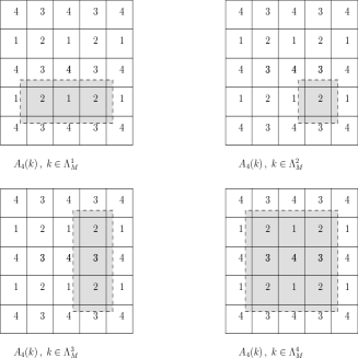
Fig. 2: The index sets $A_{4}(k)$ for $k\in{\bar{\Lambda}_{M}}^{\alpha}$, $\alpha=1,2,3,4$, $d=2$, depicted as shaded cells. The cells in each lattice are numbered by $\alpha$ denoting the sublattice ${\bar{\Lambda}_{M}}^{\alpha}$ to which the cell belongs.

General formulation. At this point we proceed with the general formulation for given $\alpha$ of the relevant quantities which are the reference measure $\nu^{\alpha}_{>\alpha}(d\sigma^{\alpha})$, the error term $\Phi^{\alpha}_{k}$, with $k\in{\bar{\Lambda}_{M}}$ and the sets $A_{\alpha}(k)$ and $B_{\alpha}(k)$, with the latter being the relevant boundary of $A_{\alpha}$. The index $\alpha$ indicates the sublattice we are considering.

Definition 7.

The sets $A_{\alpha}(k)$ and $B_{\alpha}(k)$ for $k\in{\bar{\Lambda}_{M}}^{\alpha}$ are

$$A_{\alpha}(k)=\cup_{l:\|l-k\|=1,\,p(l)\leq\alpha}C_{l}\,,\;\;\;B_{\alpha}(k)=\cup_{l:\|l-k\|=1,\,p(l)>\alpha}C_{l}\,.$$

Definition 8.

Given $\alpha=1,\ldots,2^{d}$ we define the normalized Bernoulli measure on ${\bar{\Lambda}_{M}}^{\alpha}$

$$\nu^{\alpha}_{>\alpha}(d\sigma^{\alpha})=\prod_{k\in{\bar{\Lambda}_{M}}^{\alpha}}\nu^{\alpha}_{B_{\alpha}(k)}(d\sigma^{\alpha})\,,$$ (69)

where

$$\nu^{\alpha}_{B_{\alpha}(k)}(d\sigma^{\alpha})=\frac{e^{-H^{s}_{k}(\sigma^{\alpha})}e^{-W_{k}(\sigma^{\alpha};\,\sigma^{>\alpha})}}{Z(A_{\alpha}(k);\sigma^{>\alpha};\eta(k))}Z(A_{\alpha}(k)/\{k\};\sigma^{>\alpha};\eta(k))\prod_{l\in B_{\alpha}(k)}P_{l}(d\sigma^{\alpha})\,.$$ (70)

As we have seen in Step 3 we have two kinds of error terms $\Phi^{\alpha}_{k}$, in particular, those with $k\in{\bar{\Lambda}_{M}}^{\alpha}$ and others with $k\notin{\bar{\Lambda}_{M}}^{\alpha}$. In order to describe the latter we need to introduce additional notation.

For $\alpha=1,\ldots,2^{d}$ we denote by $\Gamma_{\alpha}$ the family of parallel hyperplanes of dimension $d-1$ orthogonal to $e_{\alpha+1}$ passing through all the points $k\in{\bar{\Lambda}_{M}}^{\alpha}$. Note that for any $\alpha$, we have that ${\bar{\Lambda}_{M}}=\Gamma_{\alpha}\cup(\Gamma_{\alpha}+e_{\alpha+1})$. In the next definition we introduce a new parameter $\epsilon_{\alpha}(k)\in\{\pm 1\}$ depending on whether we should perform gluing or unfolding as discussed before. This is determined as follows: for fixed $\alpha\in{\bar{\Lambda}_{M}}$ let $d(\alpha,\beta)$ be the distance between the sublattices ${\bar{\Lambda}_{M}}^{\alpha}$ and ${\bar{\Lambda}_{M}}^{\beta}$ in the metric $\|\alpha-\beta\|_{\infty}=\sum_{i=1}^{d}|\alpha_{i}-\beta_{i}|$. Moreover, we can find orthogonal vectors $\{v_{j}\}_{j=1,\ldots,d(\alpha,\beta)}$ and a family of signs $\{\epsilon_{j}\}_{j=1,\ldots,d(\alpha,\beta)}$ such that

$${\bar{\Lambda}_{M}}^{\alpha}={\bar{\Lambda}_{M}}^{\beta}+\gamma(\alpha,\beta)\,\,\,\,\,\,\mbox{with}\,\,\,\,\,\gamma(\alpha,\beta)=\sum_{j=1}^{d(\alpha,\beta)}\epsilon_{j}\,v_{j}\,.$$

Note also that $|\gamma(\alpha,\beta)|=d(\alpha,\beta)$. Then the exponents $\epsilon_{\alpha}(k)$ with $p(k)=\beta$ are given by

$$\epsilon_{\alpha}(k):=(-1)^{|\gamma(\alpha,\beta)|}\,.$$

Furthermore, we denote by $Y(k,\gamma(\alpha,\beta))$ the affine hyperplane of codimension $|\gamma(\alpha,\beta)|$ orthogonal to the connecting vectors $\{v_{j}\}_{j=1,\ldots,|\gamma(\alpha,\beta)|}$ and passing through the point $k$

$$Y(k,\gamma(\alpha,\beta))=\cap_{j=1}^{|\gamma(\alpha,\beta)|}Y(k,v_{j})\,,$$

where $Y(k,v)$ is the hyperplane of dimension $d-1$ passing through $k$ and being perpendicular to the vector $v$. From the set of coarse-lattice points belonging to $Y(k,v)$ we define the corresponding set by

$$\mathcal{Y}(k,\gamma(\alpha,\beta)):=\cup_{l\in Y(k,\gamma(\alpha,\beta))}C_{l}\,.$$

Then, letting $k\in{\bar{\Lambda}_{M}}^{\alpha}$, for $l$ such that $C_{l}\subset\partial C_{k}$ and with $l\in{\bar{\Lambda}_{M}}^{\beta}$, for some $\beta$, we define

$$A_{\alpha}(l) = \begin{cases}\emptyset&\text{if $p(l)>2^{d(\alpha)}$}\\ A_{\alpha}(k)\cap\mathcal{Y}(l,\gamma(\alpha,\beta))&\mbox{otherwise,}\end{cases}$$ (71)

$$B_{\alpha}(l) = B_{\alpha}(k)\cap\mathcal{Y}(l,\gamma(\alpha,\beta))\,.$$ (72)

With the above definitions we can determine the error terms in the general expansion.

Definition 9.

For any $k\in{\bar{\Lambda}_{M}}^{\alpha}$ and for $k\in\Gamma_{\alpha}$ the error terms are given by

$$\Phi^{\alpha}_{k}=-1+\frac{Z(A_{\alpha}(k);\sigma^{>\alpha};\eta(k))Z(A_{\alpha+1}(k);\sigma^{>\alpha+1};\eta(k))}{(S^{+}_{k,e_{\alpha+1}}Z)(S^{-}_{k,e_{\alpha+1}}Z)}\,.$$

Moreover, if $k\in\Gamma_{\alpha}+e_{\alpha+1}$ and $k\notin{\bar{\Lambda}_{M}}^{\alpha+1}$ we have:

$$\Phi^{\alpha}_{k}=-1+\left[\frac{Z(A_{\alpha}(k);\sigma^{>\alpha};\eta(k))Z(A_{\alpha+1}(k);\sigma^{>\alpha+1};\eta(k))}{(S^{+}_{k-e_{\alpha+1},e_{\alpha+1}}Z)(S^{-}_{k+e_{\alpha+1},e_{\alpha+1}}Z)}\right]^{-\epsilon_{\alpha}(k)}\,.$$

Furthermore, if $k\in{\bar{\Lambda}_{M}}^{\alpha+1}$ we replace $Z(A_{\alpha+1}(k);\sigma^{>\alpha+1})$ by $Z(A_{\alpha+1}(k)/\{k\};\sigma^{>\alpha+1})$.

From Proposition 2.5.1 in [31] we have that the general $d$-dimensional formulation of the a priori measure induced by the short-range interactions is

$$e^{-H_{N}^{s}(\sigma)}\prod_{k\in{\bar{\Lambda}_{M}}}P_{k}(d\sigma)=R^{s}(\eta)A(\sigma)\nu(d\sigma|\eta)\,,$$

where we have the following factors

(i)

a product of partition functions (depending only on the coarse-grained variable $\eta$) over finite sets of coarse cells with supports $A_{2^{d}}(k)$, with $k\in{\bar{\Lambda}_{M}}^{\alpha}$ and $\alpha=1,\ldots,2^{d}$

$$R^{s}(\eta):=\prod_{\alpha=1}^{2^{d}}\prod_{k\in{\bar{\Lambda}_{M}}^{\alpha}}\left[Z(A_{2^{d}}(k);\,\eta(k))^{\epsilon_{2^{d}}(k)}\right]\,,$$ (73)

(ii)

error terms in the form of a gas of polymers (with the only interaction to be a hard-core exclusion)

$$A(\sigma):=\prod_{\alpha=1}^{2^{d}}\prod_{j\leq 2^{d(\alpha)}}\prod_{k\in{\bar{\Lambda}_{M}}^{j}}(1+\Phi^{\alpha}_{k})\,,$$

(iii)

a reference measure induced by only the short-range interactions once we neglect the reference system and the error terms

$$\nu(d\sigma|\eta):=\nu^{2^{d}}\ldots\nu^{2}_{>2}\nu^{1}_{>1}\,.$$

With this expansion for the short range interactions, going back to the general strategy presented in Section 3, if we also consider the long-range contribution from (15), we obtain

$$e^{-\beta\bar{H}_{M}(\eta)} = \int e^{-\beta H_{N}^{l}}e^{-\beta H_{N}^{s}}\prod_{k}P_{k}(d\sigma)$$

$$= e^{-\beta\bar{H}^{l,(0)}(\eta)}R(\eta)\int e^{-\beta(H_{N}^{l}-\bar{H}^{l,(0)})}A(\sigma)\nu(d\sigma|\eta)\,,$$

which implies that

$$\bar{H}_{M}(\eta)=\bar{H}^{l,(0)}(\eta)-\log R(\eta)-\frac{1}{\beta}\log{\mathbb{E}}_{\nu}[e^{-\beta(H_{N}^{l}-\bar{H}^{l,(0)})}A(\sigma)|\eta]\,.$$ (74)

5.1 Cluster expansion and effective interactions

The goal of this section is to expand the term ${\mathbb{E}}_{\nu}[e^{-\beta(H_{N}^{l}(\sigma)-\bar{H}^{l,(0)}(\eta))}A(\sigma)|\eta]$ in (74) into a convergent series using a cluster expansion. By the construction given previously the terms in $A(\sigma)$ are already in the form of a polymer gas with hard-core interactions only. For the long-range part we first write the difference $H_{N}^{l}(\sigma)-\bar{H}^{l,(0)}(\eta)$ as

$$H_{N}^{l}(\sigma)-\bar{H}^{l,(0)}(\eta)=\sum_{k\leq l}\Delta_{kl}J(\sigma)\,,\;\;\;\;\mbox{where}$$

$$\Delta_{kl}J(\sigma):=-\frac{1}{2}\sum_{\genfrac{}{}{0.0pt}{2}{x\in C_{k}}{y\in C_{l},y\neq x}}(J(x-y)-\bar{J}(k,l))\sigma(x)\sigma(y)(2-\delta_{kl})\,.$$ (75)

We also define $f_{kl}(\sigma):=e^{-\beta\Delta_{kl}J(\sigma)}-1$ and we obtain

$${\mathbb{E}}_{\nu}[e^{-\beta(H_{N}^{l}(\sigma)-\bar{H}^{l,(0)}(\eta)}A(\sigma)|\eta]=\int\prod_{k\leq l}(1+f_{kl})\prod_{\alpha=1}^{2^{d}}\prod_{j\leq 2^{d(\alpha)}}\prod_{k\in{\bar{\Lambda}_{M}}^{j}}(1+\Phi^{\alpha}_{k})\nu(d\sigma|\eta)\,.$$ (76)

We define the polymer model which contains combined interactions originating from both the short and long-range potential. By expanding the products in (76) we obtain terms of the type

$$\prod_{j=1}^{p}\Phi^{\alpha_{j}}_{k_{j}}\prod_{i=1}^{q}f_{l_{i},m_{i}}\,\,\,\,\,\,\mbox{where}\,\,\,k_{j},l_{i},m_{i}\in{\bar{\Lambda}_{M}}\,\,\,\mbox{and}\,\,\,\alpha_{j}\in\{1,\ldots,2^{d}\}$$

for some $p$ and $q$. The factors $\Phi^{\alpha_{j}}_{k_{j}}$ are functions of the variables which are on the boundary of the corresponding sets $A_{\alpha_{j}}(k_{j})$. This boundary is described by the set

$$C_{0}^{\alpha}(k)=\begin{cases}B_{\alpha}(k)&\text{if $k\in\Gamma_{\alpha}$,}\\ B_{\alpha+1}(k)&\text{if $k\in\Gamma_{\alpha}+e_{\alpha+1}$.}\end{cases}$$ (77)

Furthermore, since the measure $\nu(d\sigma|\eta)$ is not a product measure but instead a composition of measures each one parametrized by variables which are integrated by the next measure, we need to create a “safety” corridor around the sets $C_{0}^{\alpha}$ depending on the level of $\alpha$. This is given in the next definition. For a given integer $\beta$, with $1<\beta<2^{d}-\alpha$ we define

$$C_{\beta}^{\alpha}(k)=\cup_{\epsilon_{1},\ldots,\epsilon_{\beta}\in\{\pm 1\}^{\beta}}\cup_{l:C_{l}\subset\partial(C_{k+\epsilon_{1}e_{\alpha+1}+\ldots+\epsilon_{\beta}e_{\alpha+\beta}}),\,p(l)>\alpha+\beta}C_{l}\,,$$ (78)

Then for given $\alpha\in\{1,\ldots,2^{d}\}$ we call a “bond” of type $C^{\alpha}$ the set

$$C^{\alpha}(k)=\cup_{\beta=0}^{2^{d}-\alpha}C_{\beta}^{\alpha}(k)\,.$$ (79)

With this definition, any factor $\Phi^{\alpha_{j}}_{k_{j}}$ has a region of dependence which is given by the bond $C^{\alpha}(k)$. Similarly, for the factors $f_{l_{i},m_{i}}$ originating from the long-range interactions the initial domain of dependence is $C_{l_{i}}\cup C_{m_{i}}$. However, due to the non-product structure of the measure we need to introduce a safety corridor in the same way. Given $k\in{\bar{\Lambda}_{M}}$ for $\beta$ an integer with $1<\beta<2^{d}-p(k)$ we define

$$C_{\beta}(k)=\cup_{\epsilon_{1},\ldots,\epsilon_{\beta}\in\{\pm 1\}^{\beta}}\cup_{l:C_{l}\subset\partial(C_{k+\epsilon_{1}e_{\alpha+1}+\ldots+\epsilon_{\beta}e_{\alpha+\beta}}),\,p(l)>p(k)+\beta}C_{l}\,.$$ (80)

Then for a given $f_{kl}$ we define

$$C(k,l)=\cup_{\beta=1}^{2^{d}-p(k)}C_{\beta}(k)\cup_{\beta=1}^{2^{d}-p(l)}C_{\beta}(l)\,.$$ (81)

With a slight abuse of notation we define for $R_{0}=\{k_{1},\ldots,k_{|R_{0}|}\}$

$$C(R_{0})=\cup_{i=1}^{|R_{0}|}\cup_{\beta=1}^{2^{d}-p(k_{i})}C_{\beta}(k_{i})\,.$$ (82)

A bond $l$ will be either a $C^{\alpha}_{k}$ bond for some $\alpha,k$, called of type $1$, or any subset of ${\bar{\Lambda}_{M}}$, we call it a bond of type $2$. We say that two bonds $l_{1}$ and $l_{2}$ are connected if $l_{1}\cap l_{2}\neq\emptyset$. We call a polymer $R$ a set of bonds $l_{1},\ldots,l_{p},l_{p+1}$ where $l_{1},\ldots,l_{p}$ are bonds of type $1$ and $l_{p+1}$ is a bond of type $2$, i.e., a possibly empty subset $R_{0}\subset{\bar{\Lambda}_{M}}$. A polymer is called connected if for all $i,j$, with $1\leq i<j\leq p+1$, there exists a chain of connected bonds in $R$ joining $l_{i}$ to $l_{j}$. For such a polymer $R$ we define its cardinality to be two integers, the first counting the number of bonds of the type $1$ and the second being the number of coarse cells included in the bond of type $2$, i.e., $\mbox{card\,}(R):=(p,|R_{0}|)$. The support $\mbox{supp\,}(R)$ of $R$ is $\mbox{supp\,}(R)=\cup_{i=1}^{p+1}l_{i}$ where $l_{p+1}\equiv C(R_{0})$ (see (82)). Let $\mathcal{R}$ be the set of all such polymers. Two polymers $R_{1},R_{2}$ are said to be compatible if $\tilde{R}_{1}\cap\tilde{R}_{2}=\emptyset$ and we write $R_{1}\sim R_{2}$.

Given a polymer $R=l_{1},\ldots,l_{p},l_{p+1}$ we define the activity of $R$ to be the function $w:\,\mathcal{R}\to\mathbb{C}$ given by

$$w(R)=\int\nu(d\sigma|\eta)\left(\prod_{j=1}^{p}\Phi^{\alpha_{j}}_{k_{j}}\sum_{g\in\mathcal{G}_{R_{0}}}\prod_{\{k,l\}\in E(g)}f_{k,l}\right)\,,$$ (83)

where $\mathcal{G}_{l}$ is the collection of connected graphs on the vertices of $l$ (recall $l\subset{\bar{\Lambda}_{M}}$) and $E(g)$ is the set of edges of the graph $g$.

We define a new graph $\mathbb{G}$ on $\mathcal{R}$ which has the edge $R_{i}$-$R_{j}$ if the polymers $R_{i}$ and $R_{j}$ are not compatible. We call $G\subset\mathcal{R}$ completely disconnected if the subgraph induced by $\mathbb{G}$ on $G$ has no edges. Let

$$\mathcal{D}_{\mathcal{R}}=\cup_{n=0}^{|\mathcal{R}|}\{(R_{1},\ldots,R_{n})\subset\mathcal{R}:\,\forall i\neq j,\,R_{i}\sim R_{j}\,,\}$$

then the partition function $Z$ can be written as

$$Z=\sum_{G\in\mathcal{D}_{\mathcal{R}}}\prod_{R\in G}w(R)\,,$$

which is the abstract form of a polymer model. Thus we can apply the general theorem of the cluster expansion once we check the convergence condition. The condition is stated as a theorem in [4].

Theorem 10 ([4]).

Let $a:\mathcal{R}\to\mathbb{R}_{+}$. Consider the subset of $\mathbb{C}^{\mathcal{R}}$

$$\mathcal{P}_{\mathcal{R}}^{a} := \{w(R),\,R\in\mathcal{R}:\,\forall\,R\in\mathcal{R}:\,\,|w(R)|e^{a(R)}<1\,\rm{and}$$

$$\sum_{R^{\prime}\nsim R}(-\log(1-|w(R^{\prime})|e^{a(R^{\prime})}))\leq a(R)\}\,.$$

Then on $\mathcal{P}_{\mathcal{R}}^{a}$, $\log Z$ is well defined and analytic and

$$\log Z=\sum_{I\in\mathcal{I}(\mathcal{R})}c_{I}\prod_{R\in\rm{supp}(I)}w(R)^{I_{R}}\,,$$

where $I=(I_{R})_{R\in\mathcal{R}}$, $\mathcal{I}(\mathcal{R})$ is the collection of all multi-indexes $I$, i.e., integer valued functions on $\mathcal{R}$, and

$$c_{I}=\frac{1}{I_{R_{1}}!\ldots I_{R_{|\mathcal{R}|}}!}\frac{\partial^{I_{R_{1}}+\ldots+I_{R_{|\mathcal{R}|}}}\log Z}{\partial^{I_{R_{1}}}w(R_{1})\ldots\partial^{I_{R_{|\mathcal{R}|}}}w(R_{|\mathcal{R}|})}|_{\{w(R_{i})=0\}_{i}}\,.$$

For the proof we refer to [4]. Thus we need to check the condition of convergence. The following estimate for the long-range potential was proved in [22].

Lemma 11.

Assume that $J$ satisfies (2). Then there exists a constant $C_{1}\sim\frac{q^{d+1}}{L}\|\nabla V\|_{\infty}$ such that

$$\sup_{k\in{\bar{\Lambda}_{M}}}\sum_{l:\,l\neq k}|\Delta_{kl}J(\sigma)|\leq C_{1}\,,$$ (84)

for every $\sigma$.

For the short-range interaction we follow the analysis of [31] and we consider the following condition

Condition 5.1.

Let $e$ be a vector in one of the directions of the lattice ${\bar{\Lambda}_{M}}$ and $Z_{U}(\Lambda;\sigma_{-},\sigma_{+},\tau;\eta_{V})$ be the partition function for the interaction $U$ in the space domain $\Lambda$. We consider boundary conditions $\sigma_{\pm}$ in the directions $\pm e$ and $\tau$ in all other directions. Moreover, we impose multi-canonical constraints $\eta(k)$ for $k\in V\subset{\bar{\Lambda}_{M}}$ with $\Lambda=\cup_{k\in V}C_{k}$. For a given $q>r_{0}$, with $|C_{k}|=q^{d}$, the following inequality holds

$$\sup_{\sigma_{\pm},\tau}\sup_{\Lambda}\sup_{\eta_{V}}\Big{|}\frac{Z_{U}(\Lambda;\sigma_{-},\sigma_{+},\tau;\eta_{V})Z_{U}(\Lambda;0,0,\tau;\eta_{V})}{Z_{U}(\Lambda;0,\sigma_{+},\tau;\eta_{V})Z_{U}(\Lambda;\sigma_{-},0,\tau;\eta_{V})}-1\Big{|}\leq C_{2}\,,$$

where given the numbers $r=2^{2d}[3(2^{d+1}+1)]^{d}$, $E=2^{d+1}+1$, and $c>0$ the upper bound $C_{2}$ satisfies

$$rC_{2}e^{cE}<1\,.$$

Notice that we work with the same condition as Condition $C_{L}$ defined in [31], where in our notation $L$ is $q$, yet similar analysis applies in order to prove convergence of the cluster expansion under the milder condition Condition $C_{L}^{\prime}$ again as in [31]. We skip the analysis of such issues since it goes beyond the goal of the present work. Furthermore, these conditions are related to the ones presented in [10] in order to ensure that a given system belongs to the class of completely analytical interactions. For further details we refer the reader to [30] and [3] and to the references therein.

Now we are ready to prove the convergence condition.

Lemma 12.

The set $\mathcal{P}_{\mathcal{R}}^{a}$ is nonempty.

Proof: We take $a(R)=c|\mbox{supp\,}(R)|$, where $c$ is a constant to be chosen later. Note that $-\log(1-x)\leq 2x$, so it suffices to show that

$$\sum_{R^{\prime}\nsim R}2|w(R^{\prime})|e^{a(R^{\prime})}\leq a(R)\,.$$

Suppose that the generic polymer $R^{\prime}$ is given by $R^{\prime}=l_{1},\ldots,l_{p},l_{p+1}$, for some $p\geq 0$, where $l_{j}\equiv C^{\alpha_{j}^{\prime}}(k_{j}^{\prime})$ for $j=1,\ldots,p$ and $l_{p+1}=R_{0}^{\prime}$, with $|R_{0}^{\prime}|=n$ for some $n\geq 0$. For $|w(R^{\prime})|$ we have

$$|w(R^{\prime})|\leq\int\nu(d\sigma|\eta)\prod_{j=1}^{p}|\Phi^{\alpha_{j}}_{k_{j}}|\cdot|\sum_{g\in\mathcal{G}_{R_{0}^{\prime}}}\prod_{\{k,l\}\in E(g)}f_{kl}|\,.$$

By the graph-tree inequality we have that for all $\sigma$, $\eta$ and with $|R_{0}^{\prime}|=n$

$$|\sum_{g\in\mathcal{G}_{R_{0}^{\prime}}}\prod_{\{k,l\}\in E(g)}f_{kl}|\leq\beta 2^{n}e^{nC_{1}}\sum_{\tau^{0}\in\mathcal{T}^{0}_{n}}\prod_{\{k,l\}\in\tau^{0}}|\Delta_{kl}J(\sigma)|\,,$$

where from Lemma 11 we have that $C_{1}\sim\frac{q^{d+1}}{L}\|\nabla V\|_{\infty}$. We also let $\sup_{\sigma}|\Delta_{kl}J(\sigma)|\leq\Delta_{kl}$ with $\Delta_{kl}\equiv q^{2d}\frac{1}{L^{d}}\frac{q}{L}\|\nabla V\|_{\infty}1_{(k,l):\,|l-k|\leq\frac{L}{q}}$. Moreover, from Condition 5.1 we have

$$\int\nu(d\sigma|\eta)\prod_{j=1}^{p}|\Phi^{\alpha_{j}}_{k_{j}}|\leq(C_{2})^{p}\,.$$

Then for the activity $w(R^{\prime})$ we obtain

$$|w(R^{\prime})|\leq\beta 2^{n}e^{nC_{1}}\sum_{\tau^{0}\in\mathcal{T}^{0}_{n}}\prod_{\{k,l\}\in\tau^{0}}\Delta_{kl}\cdot(C_{2})^{p}\,.$$

Thus to satisfy the sufficient condition for the convergence of the cluster expansion we first bound the sum $\sum_{R^{\prime}\nsim R}$ by

$$\sup_{k\in R^{\prime}}|\mbox{supp\,}(R^{\prime})|\sum_{p\geq 0}\sum_{n\geq 0}\sum_{\genfrac{}{}{0.0pt}{2}{R^{\prime}:\,\mbox{supp\,}(R^{\prime})\supset\{k\},}{\mbox{card\,}(R^{\prime})=(p,n)}}\,.$$

The fixed coarse cell $C_{k}$ may belong to one of the $l_{j}$’s for $j=1,\ldots,p$ or to $R_{0}^{\prime}$. In the first case we estimate the sum over $R^{\prime}$ by

$$\sum_{\genfrac{}{}{0.0pt}{2}{l_{1}:\,l_{1}\supset\{k\}}{l_{2},\ldots,l_{p}}}\frac{1}{(p-1)!}\sum_{\genfrac{}{}{0.0pt}{2}{k_{1}\in\,(\cup_{j}l_{j})\cap R_{0}^{\prime}}{k_{2},\ldots,k_{n}}}\frac{1}{(n-1)!}\,,$$

and in the second by

$$\sum_{\genfrac{}{}{0.0pt}{2}{k_{1}=k}{k_{2},\ldots,k_{n}}}\frac{1}{(n-1)!}\sum_{\genfrac{}{}{0.0pt}{2}{l_{1}:\,l_{1}\cap R_{0}^{\prime}\neq\emptyset}{l_{2},\ldots,l_{p}}}\frac{1}{(p-1)!}\,.$$

Next, for every tree $\tau^{0}$ we have that

$$\sup_{k\in R^{\prime}}\sum_{\genfrac{}{}{0.0pt}{2}{k_{1}=k}{k_{2},\ldots,k_{n}}}\prod_{i,j\in\tau^{0}}\Delta_{k_{i},k_{j}}\leq C_{1}^{n-1}\,.$$

We use the Cayley formula $\sum_{\tau^{0}\in\mathcal{T}^{0}_{n}}1=n^{n-2}$ and the fact that the cardinality of the sum $\sum_{\genfrac{}{}{0.0pt}{2}{l_{1}:\,l_{1}\supset\{k\}}{l_{2},\ldots,l_{p}}}$ can be bounded by $r^{p}$, where $r=2^{2d}[3(2^{d+1}+1)]^{d}$ is an upper bound for the maximum number of $C^{\alpha}$ bonds that can pass through a point, as showed in [31]. Taking into account all the above we obtain

$$\sum_{R^{\prime}\nsim R}2|w(R^{\prime})|e^{a(R^{\prime})} \leq |\mbox{supp\,}(R^{\prime})|\sum_{n\geq 1}A_{1}(n)\sum_{p\geq 1}A_{2}(p)\,,$$

where

$$A_{1}(n)=\frac{1}{(n-1)!}n^{n-2}(\beta C_{1})^{n-1}2^{n}e^{n\beta C_{1}}e^{cn}\,\,\,\,\,\,\,\mathrm{and}\,\,\,\,\,A_{2}(p)=\frac{1}{(p-1)!}r^{p}C_{2}^{p}e^{cEp}\,,$$

and $E$ is the upper bound for the cardinality of any bond $C^{\alpha}(k)$, i.e.,

$$\sup_{\alpha=1,\ldots,2^{d}}\sup_{k\in{\bar{\Lambda}_{M}}^{\alpha}}|C^{\alpha}(k)|\leq E\equiv 2^{d+1}+1\,.$$

For $C_{1}$ and $C_{2}$ sufficiently small the two series converge to a finite number and we choose $c$ to be this number. $\Box$

References

- [1] Reinier L. C. Akkermans and W. J. Briels. Coarse-grained interactions in polymer melts: A variational approach. J. Chem. Phys., 115(13):6210–6219, 2001.
- [2] S. Are, M. A. Katsoulakis, P. Plecháč, and L. Rey-Bellet. Multibody interactions in coarse-graining schemes for extended systems. SIAM J. Sci. Comput., 31(2):987–1015, 2008.
- [3] L. Bertini, E. N. M. Cirillo, and E. Olivieri. Renormalization-group transformations under strong mixing conditions: Gibbsianness and convergence of renormalized interactions. J. Statist. Phys., 97(5-6):831–915, 1999.
- [4] A. Bovier and M. Zahradník. A simple inductive approach to the problem of convergence of cluster expansions of polymer models. J. Statist. Phys., 100(3-4):765–778, 2000.
- [5] M. Cassandro and E. Presutti. Phase transitions in Ising systems with long but finite range interactions. Markov Process. Related Fields, 2(2):241–262, 1996.
- [6] A. Chatterjee, M. Katsoulakis, and D. Vlachos. Spatially adaptive lattice coarse-grained Monte Carlo simulations for diffusion of interacting molecules. J. Chem. Phys., 121(22):11420–11431, 2004.
- [7] A. Chatterjee, M. Katsoulakis, and D. Vlachos. Spatially adaptive grand canonical ensemble Monte Carlo simulations. Phys. Rev. E, 71, 2005.
- [8] A. Chatterjee and D.G. Vlachos. An overview of spatial microscopic and accelerated kinetic monte carlo methods. J. Comput-Aided Mater. Des., 14(2):253–308, 2007.
- [9] Jianguo Dai, W. D. Seider, and T. Sinno. Coarse-grained lattice kinetic Monte Carlo simulation of systems of strongly interacting particles. J. Chem. Phys., 128(19):194705, 2008.
- [10] R. L. Dobrushin and S. B. Shlosman. Completely analytical interactions: constructive description. J. Statist. Phys., 46(5-6):983–1014, 1987.
- [11] E. Espanol, M. Serrono, and Zuniga. Coarse-grainiing of a fluid and its relation with dissipasive particle dynamics and smoothed particle dynamics. Int. J. Modern Phys. C, 8(4):899–908, 1997.
- [12] P. Espanol and P. Warren. Statistics-mechanics of dissipative particle dynamics. Europhys. Lett., 30(4):191–196, 1995.
- [13] Francesca Fierro and Andreas Veeser. On the a posteriori error analysis for equations of prescribed mean curvature. Math. Comp., 72(244):1611–1634, 2003.
- [14] H. Fukunaga, J. Takimoto, and M. Doi. A coarse-graining procedure for flexible polymer chains with bonded and nonbonded interactions. J. Chem. Phys., 116(18):8183–8190, 2002.
- [15] N. Goldenfeld. Lectures on Phase Transitions and the Renormalization Group, volume 85. Addison-Wesley, New York, 1992.
- [16] G. Hadjipanayis, editor. Magnetic Hysteresis in Novel Magnetic Materials, volume 338 of NATO ASI Series E, Dordrecht, The Netherlands, 1997. Kluwer Academic Publishers.
- [17] V.A. Harmandaris, N.P. Adhikari, N.F.A. van der Vegt, and K. Kremer. Hierarchical modeling of polystyrene: From atomistic to coarse-grained simulations. Macromolecules, 39:6708–6719, 2006.
- [18] L. Kadanoff. Scaling laws for Ising models near . Physics, 2:263, 1966.
- [19] M. A. Katsoulakis, A. J. Majda, and D. G. Vlachos. Coarse-grained stochastic processes and Monte Carlo simulations in lattice systems. J. Comp. Phys., 186:250–278, 2003.
- [20] M. A. Katsoulakis, L. Rey-Bellet, P. Plecháč, and D. K.Tsagkarogiannis. Mathematical strategies in the coarse-graining of extensive systems: error quantification and adaptivity. J. Non Newt. Fluid Mech., 152:101–112, 2008.
- [21] Markos A. Katsoulakis, Petr Plecháč, and Luc Rey-Bellet. Numerical and statistical methods for the coarse-graining of many-particle stochastic systems. J. Sci. Comput., 37(1):43–71, 2008.
- [22] Markos A. Katsoulakis, Petr Plecháč, Luc Rey-Bellet, and Dimitrios K. Tsagkarogiannis. Coarse-graining schemes and a posteriori error estimates for stochastic lattice systems. M2AN Math. Model. Numer. Anal., 41(3):627–660, 2007.
- [23] Markos A. Katsoulakis, Petr Plecháč, and Alexandros Sopasakis. Error analysis of coarse-graining for stochastic lattice dynamics. SIAM J. Numer. Anal., 44(6):2270–2296, 2006.
- [24] Markos A. Katsoulakis and José Trashorras. Information loss in coarse-graining of stochastic particle dynamics. J. Stat. Phys., 122(1):115–135, 2006.
- [25] K. Kremer and F. Muller-Plathe. Multiscale problems in polymer science: Simulation approaches. MRS Bulletin, 26(3):205–210, 2001.
- [26] O. Lakkis and R. H. Nochetto. A posteriori error analysis for the mean curvature flow of graphs. SIAM J. Numer. Anal., 42(5):1875–1898, 2005.
- [27] D. Landau and K. Binder. A Guide to Monte Carlo Simulations in Statistical Physics. Cambridge University Press, 2000.
- [28] A. P. Lyubartsev, M. Karttunen, P. Vattulainen, and A. Laaksonen. On coarse-graining by the inverse monte carlo method: Dissipative particle dynamics simulations made to a precise tool in soft matter modeling. Soft Materials, 1(1):121–137, 2003.
- [29] F. Müller-Plathe. Coarse-graining in polymer simulation: from the atomistic to the mesoscale and back. Chem. Phys. Chem., 3:754, 2002.
- [30] E. Olivieri. On a cluster expansion for lattice spin systems: a finite-size condition for the convergence. J. Statist. Phys., 50(5-6):1179–1200, 1988.
- [31] E. Olivieri and P. Picco. Cluster expansion for -dimensional lattice systems and finite-volume factorization properties. J. Statist. Phys., 59(1-2):221–256, 1990.
- [32] I. Pivkin and G. Karniadakis. Coarse-graining limits in open and wall-bounded dissipative particle dynamics systems. J. Chem. Phys., 124:184101, 2006.
- [33] R. Plass, J.A. Last, N.C. Bartelt, and G.L. Kellogg. Self-assembled domain patterns. Nature, 412:875, 2001.
- [34] M. Praprotnik, S. Matysiak, L. Delle Site, K. Kremer, and C. Clementi. Adaptive resolution simulation of liquid water. J. Physics: Condensed Matter, 19(29):292201 (10pp), 2007.
- [35] M. Seul and D. Andelman. Domain shapes and patterns: the phenomenology of modulated phases. Science, 267:476–483, 1995.
- [36] B. Simon. The Statistical Mechanics of Lattice Gases, vol. I. Princeton series in Physics, 1993.
- [37] J. Trashorras and D. K. Tsagkarogiannis. Reconstruction schemes for coarse-grained stochastic lattice systems. preprint, 2008. submitted.
- [38] W. Tschöp, K. Kremer, O. Hahn, J. Batoulis, and T. Bürger. Simulation of polymer melts. II. from coarse-grained models back to atomistic description. Acta Polym., 49:75, 1998.
- [39] G.A. Voth. Coarse-Graining of Condensed Phase and Biomolecular Systems. CRC Press, Boca Raton, FL, 2009.