Firefly Algorithm, Lévy Flights and Global Optimization

Abstract

Nature-inspired algorithms such as Particle Swarm Optimization and Firefly Algorithm are among the most powerful algorithms for optimization. In this paper, we intend to formulate a new metaheuristic algorithm by combining Lévy flights with the search strategy via the Firefly Algorithm. Numerical studies and results suggest that the proposed Lévy-flight firefly algorithm is superior to existing metaheuristic algorithms. Finally implications for further research and wider applications will be discussed.

Citation detail: X.-S. Yang,“Firefly algorithm, Lévy flights and global optimization”, in: Research and Development in Intelligent Systems XXVI (Eds M. Bramer, R. Ellis, M. Petridis), Springer London, pp. 209-218 (2010).

1 Introduction

Nature-inspired metaheuristic algorithms are becoming powerful in solving modern global optimization problems [2, 3, 5, 7, 9, 18, 17], especially for the NP-hard optimization such as the travelling salesman problem. For example, particle swarm optimization (PSO) was developed by Kennedy and Eberhart in 1995 [8, 9], based on the swarm behaviour such as fish and bird schooling in nature. It has now been applied to find solutions for many optimization applications. Another example is the Firefly Algorithm developed by the author [18] which has demonstrated promising superiority over many other algorithms. The search strategies in these multi-agent algorithms are controlled randomization, efficient local search and selection of the best solutions. However, the randomization typically uses uniform distribution or Gaussian distribution.

On the other hand, various studies have shown that flight behaviour of many animals and insects has demonstrated the typical characteristics of Lévy flights [4, 13, 11, 12]. A recent study by Reynolds and Frye shows that fruit flies or Drosophila melanogaster, explore their landscape using a series of straight flight paths punctuated by a sudden $90^{\o}$ turn, leading to a Lévy-flight-style intermittent scale free search pattern. Studies on human behaviour such as the Ju/’hoansi hunter-gatherer foraging patterns also show the typical feature of Lévy flights. Even light can be related to Lévy flights [1]. Subsequently, such behaviour has been applied to optimization and optimal search, and preliminary results show its promising capability [11, 13, 15, 16].

This paper aims to formulate a new Lévy-flight Firefly Algorithm (LFA) and to provide the comparison study of the LFA with PSO and other relevant algorithms. We will first outline the firefly algorithms, then formulate the Lévy-flight FA and finally give the comparison about the performance of these algorithms. The LFA optimization seems more promising than particle swarm optimization in the sense that LFA converges more quickly and deals with global optimization more naturally. In addition, particle swarm optimization is just a special class of the LFA as we will demonstrate this in this paper.

2 Firefly Algorithm

2.1 Behaviour of Fireflies

The flashing light of fireflies is an amazing sight in the summer sky in the tropical and temperate regions. There are about two thousand firefly species, and most fireflies produce short and rhythmic flashes. The pattern of flashes is often unique for a particular species. The flashing light is produced by a process of bioluminescence, and the true functions of such signaling systems are still debating. However, two fundamental functions of such flashes are to attract mating partners (communication), and to attract potential prey. In addition, flashing may also serve as a protective warning mechanism. The rhythmic flash, the rate of flashing and the amount of time form part of the signal system that brings both sexes together. Females respond to a male’s unique pattern of flashing in the same species, while in some species such as photuris, female fireflies can mimic the mating flashing pattern of other species so as to lure and eat the male fireflies who may mistake the flashes as a potential suitable mate.

The flashing light can be formulated in such a way that it is associated with the objective function to be optimized, which makes it possible to formulate new optimization algorithms. In the rest of this paper, we will first outline the basic formulation of the Firefly Algorithm (FA) and then discuss the implementation as well as analysis in detail.

2.2 Firefly Algorithm

Now we can idealize some of the flashing characteristics of fireflies so as to develop firefly-inspired algorithms. For simplicity in describing our Firefly Algorithm (FA), we now use the following three idealized rules: 1) all fireflies are unisex so that one firefly will be attracted to other fireflies regardless of their sex; 2) Attractiveness is proportional to their brightness, thus for any two flashing fireflies, the less brighter one will move towards the brighter one. The attractiveness is proportional to the brightness and they both decrease as their distance increases. If there is no brighter one than a particular firefly, it will move randomly; 3) The brightness of a firefly is affected or determined by the landscape of the objective function. For a maximization problem, the brightness can simply be proportional to the value of the objective function. Other forms of brightness can be defined in a similar way to the fitness function in genetic algorithms or the bacterial foraging algorithm (BFA) [6, 10].

In the firefly algorithm, there are two important issues: the variation of light intensity and formulation of the attractiveness. For simplicity, we can always assume that the attractiveness of a firefly is determined by its brightness which in turn is associated with the encoded objective function.

In the simplest case for maximum optimization problems, the brightness $I$ of a firefly at a particular location ${\bf x}$ can be chosen as $I({\bf x})\propto f({\bf x})$. However, the attractiveness $\beta$ is relative, it should be seen in the eyes of the beholder or judged by the other fireflies. Thus, it will vary with the distance $r_{ij}$ between firefly $i$ and firefly $j$. In addition, light intensity decreases with the distance from its source, and light is also absorbed in the media, so we should allow the attractiveness to vary with the degree of absorption. In the simplest form, the light intensity $I(r)$ varies according to the inverse square law $I(r)=\frac{I_{s}}{r^{2}}$ where $I_{s}$ is the intensity at the source. For a given medium with a fixed light absorption coefficient $\gamma$, the light intensity $I$ varies with the distance $r$. That is

$$I=I_{0}e^{-\gamma r},$$ (1)

where $I_{0}$ is the original light intensity.

As a firefly’s attractiveness is proportional to the light intensity seen by adjacent fireflies, we can now define the attractiveness $\beta$ of a firefly by

$$\beta=\beta_{0}e^{-\gamma r^{2}},$$ (2)

where $\beta_{0}$ is the attractiveness at $r=0$.

3 Lévy-Flight Firefly Algorithm

If we combine the three idealized rules with the characteristics of Lévy flights, we can formulate a new Lévy-flight Firefly Algorithm (LFA) which can be summarized as the pseudo code shown in Fig. 1.

Lévy-Flight Firefly Algorithm   begin
 Objective function $f({\bf x}),\qquad{\bf x}=(x_{1},...,x_{d})^{T}$
 Generate initial population of fireflies ${\bf x}_{i}\;(i=1,2,...,n)$
 Light intensity $I_{i}$ at ${\bf x}_{i}$ is determined by $f({\bf x}_{i})$
 Define light absorption coefficient $\gamma$
 while ($t<$MaxGeneration)
 for $i=1:n$ all $n$ fireflies
  for $j=1:i$ all $n$ fireflies
    if ($I_{j}>I_{i}$)
    Move firefly $i$ towards $j$ in d-dimension via Lévy flights
    end if
    Attractiveness varies with distance $r$ via $\exp[-\gamma r]$
    Evaluate new solutions and update light intensity
  end for $j$
 end for $i$
 Rank the fireflies and find the current best
 end while
 Postprocess results and visualization
end  

Figure 1: Pseudo code of the Lévy-Flight Firefly Algorithm (LFA).

In the implementation, the actual form of attractiveness function $\beta(r)$ can be any monotonically decreasing functions such as the following generalized form

$$\beta(r)=\beta_{0}e^{-\gamma r^{m}},\qquad(m\geq 1).$$ (3)

For a fixed $\gamma$, the characteristic length becomes $\Gamma=\gamma^{-1/m}\rightarrow 1$ as $m\rightarrow\infty$. Conversely, for a given length scale $\Gamma$ in an optimization problem, the parameter $\gamma$ can be used as a typical initial value. That is $\gamma=\frac{1}{\Gamma^{m}}$.

The distance between any two fireflies $i$ and $j$ at ${\bf x}_{i}$ and ${\bf x}_{j}$, respectively, is the Cartesian distance

$$r_{ij}=||{\bf x}_{i}-{\bf x}_{j}||=\sqrt{\sum_{k=1}^{d}(x_{i,k}-x_{j,k})^{2}},$$ (4)

where $x_{i,k}$ is the $k$th component of the spatial coordinate ${\bf x}_{i}$ of $i$th firefly. For other applications such as scheduling, the distance can be time delay or any suitable forms.

The movement of a firefly $i$ is attracted to another more attractive (brighter) firefly $j$ is determined by

$${\bf x}_{i}={\bf x}_{i}+\beta_{0}e^{-\gamma r^{2}_{ij}}({\bf x}_{j}-{\bf x}_{i})+\alpha\;\textrm{sign}[{\rm rand}-\frac{1}{2}]\oplus\textrm{L\'{e}vy},$$ (5)

where the second term is due to the attraction while the third term is randomization via Lévy flights with $\alpha$ being the randomization parameter. The product $\oplus$ means entrywise multiplications. The sign[rand-$\frac{1}{2}$] where rand $\in[0,1]$ essentially provides a random sign or direction while the random step length is drawn from a Lévy distribution

$$\textrm{L\'{e}vy}\sim u=t^{-\lambda},\qquad(1<\lambda\leq 3),$$ (6)

which has an infinite variance with an infinite mean. Here the steps of firefly motion is essentially a random walk process with a power-law step-length distribution with a heavy tail.

3.1 Choice of Parameters

For most cases in our implementation, we can take $\beta_{0}=1$, $\alpha\in[0,1]$, $\gamma=1$, and $\lambda=1.5$. In addition, if the scales vary significantly in different dimensions such as $-10^{5}$ to $10^{5}$ in one dimension while, say, $-0.001$ to $0.01$ along the other, it is a good idea to replace $\alpha$ by $\alpha S_{k}$ where the scaling parameters $S_{k}(k=1,...,d)$ in the $d$ dimensions should be determined by the actual scales of the problem of interest.

The parameter $\gamma$ now characterizes the variation of the attractiveness, and its value is crucially important in determining the speed of the convergence and how the FA algorithm behaves. In theory, $\gamma\in[0,\infty)$, but in practice, $\gamma=O(1)$ is determined by the characteristic length $\Gamma$ of the system to be optimized. Thus, in most applications, it typically varies from $0.01$ to $100$.

3.2 Asymptotic Cases

There are two important limiting cases when $\gamma\rightarrow 0$ and $\gamma\rightarrow\infty$. For $\gamma\rightarrow 0$, the attractiveness is constant $\beta=\beta_{0}$ and $\Gamma\rightarrow\infty$, this is equivalent to say that the light intensity does not decrease in an idealized sky. Thus, a flashing firefly can be seen anywhere in the domain. Thus, a single (usually global) optimum can easily be reached. This corresponds to a special case of particle swarm optimization (PSO) discussed earlier. Subsequently, the efficiency of this special case is the same as that of PSO.

On the other hand, the limiting case $\gamma\rightarrow\infty$ leads to $\Gamma\rightarrow 0$ and $\beta(r)\rightarrow\delta(r)$ (the Dirac delta function), which means that the attractiveness is almost zero in the sight of other fireflies or the fireflies are short-sighted. This is equivalent to the case where the fireflies fly in a very foggy region randomly. No other fireflies can be seen, and each firefly roams in a completely random way. Therefore, this corresponds to the completely random search method.

As the Lévy-flight firefly algorithm is usually in somewhere between these two extremes, it is possible to adjust the parameters $\gamma$, $\lambda$ and $\alpha$ so that it can outperform both the random search and PSO. In fact, LFA can find the global optima as well as all the local optima simultaneously in a very effective manner.

4 Simulations and Results

4.1 Validation

In order to validate the proposed algorithm, we have implemented it in Matlab. In our simulations, the values of the parameters are $\alpha=0.2$, $\gamma=1$, $\lambda=1.5$, and $\beta_{0}=1$.

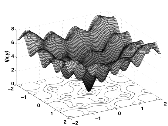
Figure 2: Ackley function for two independent variables with a global minimum $f_{*}=0$ at $(0,0)$.

As an example, we now use the LFA to find the global optimum of the Ackley function

$$f({\bf x})=-20\exp\Big{[}-\frac{1}{5}\sqrt{\frac{1}{d}\sum_{i=1}^{d}x_{i}^{2}}\Big{]}-\exp[\frac{1}{d}\sum_{i=1}^{d}\cos(2\pi x_{i})]+20+e,$$ (7)

which has a global minimum $f_{*}=0$ at $(0,0,...,0)$. The 2D Ackley function is shown in Fig. 2, and this global minimum can be found after about 200 evaluations for 40 fireflies after 5 iterations as shown in Fig. 3.

Now let us use the LFA to find the optima of some tougher test functions. For example, the author introduced a forest function [19]

$$f({\bf x})=\Big{(}\sum_{i=1}^{d}|x_{i}|\Big{)}\exp\Big{[}-\sum_{i=1}^{d}\sin(x_{i}^{2})\Big{]},\;\;\;-2\pi\leq x_{i}\leq 2\pi,$$ (8)

which has a global minimum $f_{*}=0$ at $(0,0,...,0)$. The 2D Yang’s forest function is shown in Fig. 4. However, an important feature of this test function is that it is non-smooth and its derivative is not well defined at the optima $(0,0,...,0)$ as shown in Fig. 5.

4.2 Comparison of LFA with PSO and GA

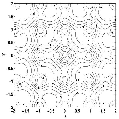
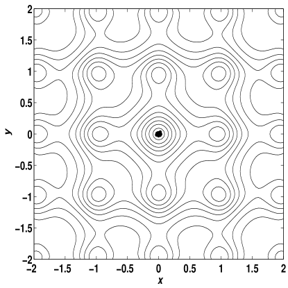
Figure 3: The initial locations of the 40 fireflies (left) and their locations after $5$ iterations (right).

Various studies show that PSO algorithms can outperform genetic algorithms (GA) [7] and other conventional algorithms for solving many optimization problems. This is partially due to that fact that the broadcasting ability of the current best estimates gives better and quicker convergence towards the optimality. A general framework for evaluating statistical performance of evolutionary algorithms has been discussed in detail by Shilane et al. [14]. Various test functions for optimization algorithms have been developed over many years, and a relatively comprehensive review of these test functions can be found in [2].

Now we will compare the LFA with PSO, and genetic algorithms for various standard test functions. We will use the same population size of $n=40$ for all algorithms in all our simulations. The PSO used is the standard version without any inertia function, while the implemented genetic algorithm has a mutation probability of $0.05$ and a crossover probability of $0.95$ without use of elitism. After implementing these algorithms using Matlab, we have carried out extensive simulations and each algorithm has been run at least 100 times so as to carry out meaningful statistical analysis. The algorithms stop when the variations of function values are less than a given tolerance $\epsilon\leq 10^{-5}$. The results are summarized in the following table (see Table 1) where the global optima are reached. The numbers are in the format: average number of evaluations (success rate), so $6922\pm 537(98\%)$ means that the average number (mean) of function evaluations is 6922 with a standard deviation of 537. The success rate of finding the global optima for this algorithm is $98\%$.

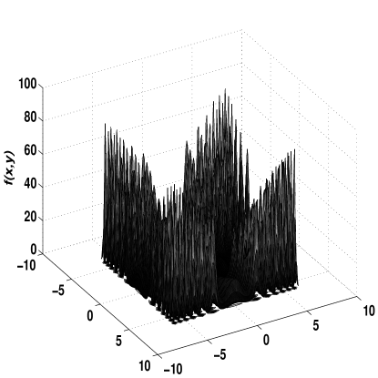
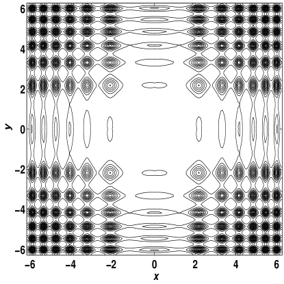
Figure 4: Yang’s forest function for two independent variables with a global minimum $f_{*}=0$ at $(0,0)$.

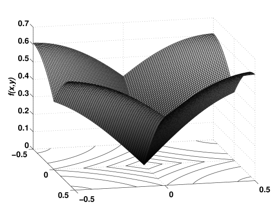
Figure 5: Non-smoothness of Yang’s forest function near the global minimum $(0,0)$.

Table 1: Comparison of algorithm performance

Functions/Algorithms	GA	PSO	LFA
Michalewicz ($d\!\!=\!\!16$)	$89325\pm 7914(95\%)$	$6922\pm 537(98\%)$	$2889\pm 719(100\%)$
Rosenbrock ($d\!\!=\!\!16$)	$55723\pm 8901(90\%)$	$32756\pm 5325(98\%)$	$6040\pm 535(100\%)$
De Jong ($d\!\!=\!\!256$)	$25412\pm 1237(100\%)$	$17040\pm 1123(100\%)$	$5657\pm 730(100\%)$
Schwefel ($d\!\!=\!\!128$)	$227329\pm 7572(95\%)$	$14522\pm 1275(97\%)$	$7923\pm 524(100\%)$
Ackley ($d\!\!=\!\!128$)	$32720\pm 3327(90\%)$	$23407\pm 4325(92\%)$	$4392\pm 2710(100\%)$
Rastrigin	$110523\pm 5199(77\%)$	$79491\pm 3715(90\%)$	$12075\pm 3750(100\%)$
Easom	$19239\pm 3307(92\%)$	$17273\pm 2929(90\%)$	$6082\pm 1690(100\%)$
Griewank	$70925\pm 7652(90\%)$	$55970\pm 4223(92\%)$	$10790\pm 2977(100\%)$
Yang	$37079\pm 8920(88\%)$	$19725\pm 3204(98\%)$	$5152\pm 2493(100\%)$
Shubert (18 minima)	$54077\pm 4997(89\%)$	$23992\pm 3755(92\%)$	$9925\pm 2504(100\%)$

We can see that the LFA is much more efficient in finding the global optima with higher success rates. Each function evaluation is virtually instantaneous on modern personal computer. For example, the computing time for 10,000 evaluations on a 3GHz desktop is about 5 seconds. Even with graphics for displaying the locations of the particles and fireflies, it usually takes less than a few minutes. Furthermore, we have used various values of the population size $n$ or the number of fireflies. We found that for most problems $n=15$ to $50$ would be sufficient. For tougher problems, larger $n$ can be used, though excessively large $n$ should not be used unless there is no better alternative, as it is more computationally extensive.

5 Conclusions

In this paper, we have formulated a new Lévy-flight firefly algorithm and analysed its similarities and differences with particle swarm optimization. We then implemented and compared these algorithms. Our simulation results for finding the global optima of various test functions suggest that particle swarm often outperforms traditional algorithms such as genetic algorithms, while LFA is superior to both PSO and GA in terms of both efficiency and success rate. This implies that LFA is potentially more powerful in solving NP-hard problems which will be investigated further in future studies.

The basic Lévy-flight firefly algorithm is very efficient. A further improvement on the convergence of the algorithm is to carry out sensitivity studies by varying various parameters such as $\beta_{0}$, $\gamma$, $\alpha$ and more interestingly $\lambda$. These could form important topics for further research. In addition, further studies on the application of FLA in combination with other algorithms may form an exciting area for further research in optimization.

References

- [1] Barthelemy, P.: Bertolotti J., Wiersma D. S., A Lévy flight for light, Nature, 453, 495-498 (2008).
- [2] Baeck, T., Fogel, D. B., Michalewicz, Z.: Handbook of Evolutionary Computation, Taylor & Francis, (1997).
- [3] Bonabeau, E., Dorigo, M., Theraulaz, G.: Swarm Intelligence: From Natural to Artificial Systems. Oxford University Press, (1999)
- [4] Brown, C., Liebovitch, L. S., Glendon, R.: Lévy flights in Dobe Ju/’hoansi foraging patterns, Human Ecol., 35, 129-138 (2007).
- [5] Deb, K., Optimisation for Engineering Design, Prentice-Hall, New Delhi, (1995).
- [6] Gazi, K., and Passino, K. M.: Stability analysis of social foraging swarms, IEEE Trans. Sys. Man. Cyber. Part B - Cybernetics, 34, 539-557 (2004).
- [7] Goldberg, D. E.: Genetic Algorithms in Search, Optimisation and Machine Learning, Reading, Mass.: Addison Wesley (1989).
- [8] Kennedy, J. and Eberhart, R. C.: Particle swarm optimization. Proc. of IEEE International Conference on Neural Networks, Piscataway, NJ. pp. 1942-1948 (1995).
- [9] Kennedy J., Eberhart R., Shi Y.: Swarm intelligence, Academic Press, (2001).
- [10] Passino, K. M.: Biomimicrt of Bacterial Foraging for Distributed Optimization, University Press, Princeton, New Jersey (2001).
- [11] Pavlyukevich, I.: Lévy flights, non-local search and simulated annealing, J. Computational Physics, 226, 1830-1844 (2007).
- [12] Pavlyukevich, I.: Cooling down Lévy flights, J. Phys. A:Math. Theor., 40, 12299-12313 (2007).
- [13] Reynolds, A. M. and Frye, M. A.: Free-flight odor tracking in Drosophila is consistent with an optimal intermittent scale-free search, PLoS One, 2, e354 (2007).
- [14] Shilane, D., Martikainen, J., Dudoit, S., Ovaska, S. J.: A general framework for statistical performance comparison of evolutionary computation algorithms, Information Sciences: an Int. Journal, 178, 2870-2879 (2008).
- [15] Shlesinger, M. F., Zaslavsky, G. M. and Frisch, U. (Eds): Lévy Flights and Related Topics in Phyics, Springer, (1995).
- [16] Shlesinger, M. F.: Search research, Nature, 443, 281-282 (2006).
- [17] Yang, X. S.: Biology-derived algorithms in engineering optimizaton (Chapter 32), in Handbook of Bioinspired Algorithms and Applications (eds Olarius & Zomaya), Chapman & Hall / CRC (2005).
- [18] Yang, X. S.: Nature-Inspired Metaheuristic Algorithms, Luniver Press, (2008).
- [19] Yang, X. S.: Engineering Optimization: An Introduction with Metaheuristic Applications, Wiley & Sons, New Jersey, (2010).