Extraction of bound-state parameters from dispersive sum rules

Abstract

The procedure of extracting the ground-state parameters from vacuum-to-vacuum and vacuum-to-hadron correlators within the method of sum rules is considered. The emphasis is laid on the crucial ingredient of this method — the effective continuum threshold. A new algorithm to fix this quantity is proposed and tested. First, a quantum-mechanical potential model which provides the only possibility to probe the reliability and the actual accuracy of the sum-rule method is used as a study case. In this model, our algorithm is shown to lead to a remarkable improvement of the accuracy of the extracted ground-state parameters compared to the standard procedures adopted in the method and used in all previous applications of dispersive sum rules in QCD. As a next step, it is demonstrated that the procedures of extracting the ground-state decay constant in the potential model and in QCD are quantitatively very close to each other. Therefore, the application of the proposed algorithm in QCD promises a considerable increase of the accuracy of the extracted hadron parameters.

1 Introduction

The method of dispersive sum rules svz ; ioffe is one of the widely used methods for obtaining properties of the ground-state hadrons in QCD. The method involves two steps: (i) one calculates the relevant correlator in QCD at relatively small values of the Euclidean time; (ii) one applies numerical procedures prompted by quark-hadron duality in order to extract the ground-state contribution from this correlator. These numerical procedures cannot determine a single value of the ground-state parameter but should provide the band of values containing the true hadron parameter with a flat probability distribution within this band svz . The width of this band is a systematic, or intrinsic, uncertainty of the method of sum rules.

It is often claimed that the standard procedures of the method of sum rules allow one to obtain hadron parameters with about 10% accuracy for normal and exotic hadrons. In many cases this is true. However, there are some examples where the difference between the sum-rule predictions and the experimental results or between the results from different versions of sum rules turn out to be quite unexpectedly much larger than 10%: as the first example, recall an evident conflict between the prediction for the $D^{*}D\pi$ coupling from light-cone sum rules belyaev and the subsequent measurement of CLEO cleo ; as the second example, mention the incompatibility of the predictions for the pion form factor at intermediate momentum transfers from light-cone sum rules braun , local-duality sum rules blm_ld , and sum rules with non-local condensates stefanis . A posteriori, these issues may be clarified. The real problem is, however, that the large errors — well exceeding a comfortable 10% level — could not be foreseen on the basis of the standard criteria adopted in the method of sum rules in QCD.

An unbiased judgement of the reliability of the extraction procedures adopted in the method of sum rules may be acquired by applying these procedures to problems where the ground-state parameters may be found independently and exactly as soon as the parameters of the theory are fixed. Presently, only quantum-mechanical potential models provide such a possibility.

A simple harmonic-oscillator (HO) potential model nsvz1 possesses two essential features of QCD — confinement and asymptotic freedom nsvz — and has the following valuable features: (i) the bound-state parameters (masses, wave functions, form factors) are known precisely; (ii) direct analogues of the QCD correlators may be calculated exactly. (For a discussion of many aspects of sum rules in quantum mechanics we refer to qmsr ; orsay ; ms_inclusive ; radyushkin2001 ).

Making use of this model, we have already studied the extraction of ground-state parameters from different types of correlators: namely, the ground-state decay constant from two-point vacuum-to-vacuum correlator lms_2ptsr , the form factor from three-point vacuum-to-vacuum correlator lms_3ptsr , and the form factor from vacuum-to-hadron correlator m_lcsr . We have demonstrated that the standard procedures adopted in the method of sum rules do not work properly: for all types of correlators the true value of the bound-state parameter was shown to lie outside the band obtained according to the standard criteria. These results gave us a solid ground to claim that also in QCD the actual accuracy of the method turns out to be worse than expected on the basis of applying the standard criteria.

We have realized that the main origin of this difficulty of the method lies in an over-simplified model for the hadron continuum, which is described as a perturbative contribution above a constant Borel-parameter-independent effective continuum threshold. We have introduced the notion of the exact effective continuum threshold, which corresponds to the true bound-state parameters: in the HO model the true hadron parameters — decay constant and form factor — are known and the exact effective continuum thresholds for different correlators may be calculated. We have demonstrated that the exact effective continuum threshold (i) is not a universal quantity and depends on the correlator considered (i.e., it is in general different for two-point and three-point correlators), (ii) depends on the Borel parameter and, for the form-factor case, also on the momentum transfer.

Moreover, we have shown that the “Borel stability criterion” combined with the assumption of a Borel-parameter-independent effective continuum threshold leads to the extraction of the wrong bound-state parameters.

In recent publications lms_prl ; lmss_lcsr ; lms_jphysg we formulated a new algorithm for extracting the parameters of the ground state. The idea proposed in these papers is to relax the standard assumption of a Borel-parameter-independent effective continuum threshold and allow for a Borel-parameter-dependent quantity.

In the present paper we develop this idea and provide details of its application to the extraction of hadron parameters from dispersive sum rules. We show that (i) the new algorithm leads to improvements — and for the case of the form factors to significant improvements — of the actual accuracy of the extracted bound-state parameters from all kinds of correlators in the potential model; (ii) the procedures of extracting the ground-state parameters from the truncated operator product expansion (OPE) for the two-point function in potential models and in QCD exhibit not only qualitative but also quantitative similarities.

The paper is organized as follows: Section 2 presents the application of our new algorithm to the extraction of the ground-state parameters from correlators in a quantum-mechanical potential model. Quantum-mechanical analogues of all correlators used in QCD for the extraction of ground-state parameters (decay constants and form factors) are discussed. Section 3 compares the extraction of the ground-state decay constant in QCD and in quantum-mechanical potential models. Section 4 presents our concluding remarks.

2 Harmonic-oscillator potential model

We consider a nonrelativistic Hamiltonian $H$ with a HO interaction potential $V(r)$, $r\equiv|{\bf r}|$:

$$H=H_{0}+V(r),\qquad H_{0}={\bf p}^{2}/2m,\qquad V(r)={m\omega^{2}r^{2}}/{2}.$$ (2.1)

In this model, all characteristics of the bound states are easily calculable. For instance, for the ground state (g), one finds

$$E_{\rm g}=\frac{3}{2}\omega,\qquad R_{\rm g}\equiv|\psi_{\rm g}({\bf r=0})|^{2}=\left(\frac{m\omega}{\pi}\right)^{3/2},\qquad F_{\rm g}(q)=\exp(-q^{2}/4m\omega),$$ (2.2)

where the elastic form factor of the ground state is defined in terms of the ground-state wave function $\psi_{\rm g}$ as

$$F_{\rm g}(q)=\langle\psi_{\rm g}|J({\bf q})|\psi_{\rm g}\rangle=\int d^{3}k\,\psi^{\dagger}_{\rm g}({\bf k})\psi_{\rm g}({\bf k-q})=\int d^{3}r\,|\psi_{\rm g}({\bf r})|^{2}e^{i{\bf qr}},\qquad q\equiv|{\bf q}|,$$ (2.3)

and the current operator $J({\bf q})$ is given by the kernel

$$\langle{\bf r^{\prime}}|J({\bf q})|{\bf r}\rangle=\exp(i{\bf qr})\delta^{(3)}({\bf r-r^{\prime}}).$$ (2.4)

2.1 Polarization operator

The quantum-mechanical analogue of the Borelized polarization operator svz has the form

$$\Pi(T)=\langle{{\bf r}_{f}=0}|\exp(-HT)|{{\bf r}_{i}=0}\rangle.$$ (2.5)

For the HO potential, the analytic expression for $\Pi(T)$ is well-known nsvz :

$$\Pi(T)=\left(\frac{\omega m}{\pi}\right)^{3/2}\frac{1}{\left[2\sinh(\omega T)\right]^{3/2}}.$$ (2.6)

Apart from the overall factor, $\Pi(T)$ is a function of one parameter $\omega T$.

Let us define the average energy of the polarization function as

$$E_{\Pi}(T)\equiv-\partial_{T}\log\Pi(T)=\frac{3}{2}\omega\coth(\omega T),\qquad\partial_{T}\equiv\frac{\partial}{\partial T}.$$ (2.7)

At $T=0$ both $\Pi(T)$ and $E_{\Pi}(T)$ diverge.

Making use of the “hadronic” bound states of the model, we obtain the following representation for $\Pi(T)$:

$$\Pi_{\rm hadr}(T)=\Pi_{\rm g}(T)+\Pi_{\rm excited}(T),\quad\Pi_{\rm g}(T)=R_{\rm g}\exp\left({-E_{\rm g}T}\right).$$ (2.8)

For large values of $T$ the contributions of the excited states to the correlator vanish and therefore $E_{\Pi}(T)\to E_{\rm g}$ for $T\to\infty$. The deviation of the energy from $E_{\rm g}$ at finite values of $T$ measures the “contamination” of the correlator by the excited states.

The OPE series is the expansion of $\Pi(T)$ at small Euclidean time $T$:

$$\Pi_{\rm OPE}(T)=\left(\frac{m}{2\pi T}\right)^{3/2}\left(1-\frac{1}{4}\omega^{2}T^{2}+\frac{19}{480}{\omega^{4}T^{4}}+\cdots\right).$$ (2.9)

For $\Pi(T)$ this expansion is equivalent to the expansion in powers of the interaction $\omega$. The first term in (2.9), $\Pi_{0}(T)$, does not depend on the interaction and describes the free propagation of the constituents. The rest of the series represents power corrections:

$$\Pi_{\rm power}(T)=\Pi_{\rm OPE}(T)-\Pi_{0}(T).$$ (2.10)

$\Pi_{0}(T)$ may be written as the spectral integral lms_2ptsr

$$\Pi_{0}(T)=\int_{0}^{\infty}dze^{-zT}\rho_{0}(z),\qquad\rho_{0}(z)=\frac{m^{3/2}}{\sqrt{2}\pi^{2}}\sqrt{z},$$ (2.11)

with $\rho_{0}(z)$ the spectral density of the one-loop two-point Feynman diagram of the nonrelativistic field theory lms_2ptsr .

2.2 Vertex function

The basic quantity for the extraction of the form factor in the method of dispersive sum rules is the correlator of three currents ioffe . The analogue of this quantity in quantum mechanics reads lms_3ptsr ; radyushkin2001

$$\Gamma(E_{2},E_{1},q)=\langle{{\bf r}_{f}=0}|(H-E_{2})^{-1}J({\bf q})(H-E_{1})^{-1}|{{\bf r}_{i}=0}\rangle,\qquad q\equiv|{\bf q}|,$$ (2.12)

[with the operator $J({\bf q})$ defined in (2.4)] and its double Borel (Laplace) transform under $E_{1}\to\tau_{1}$ and $E_{2}\to\tau_{2}$

$$\Gamma(\tau_{2},\tau_{1},q)=\langle{{\bf r}_{f}=0}|G(\tau_{2})J({\bf q})G(\tau_{1})|{{\bf r}_{i}=0}\rangle,\qquad G(\tau)\equiv\exp(-H\tau).$$ (2.13)

For large $\tau_{1}$ and $\tau_{2}$ the correlator is dominated by the ground state:

$$\Gamma(\tau_{2},\tau_{1},q)\to|\psi_{\rm g}({{\bf r}=0})|^{2}e^{-E_{\rm g}(\tau_{1}+\tau_{2})}F_{\rm g}(q^{2})+\cdots.$$ (2.14)

Let us notice the Ward identity which relates the vertex function at zero momentum to the polarization operator:

$$\Gamma(\tau_{2},\tau_{1},q=0)=\Pi(\tau_{1}+\tau_{2}).$$ (2.15)

This expression follows directly from the current-conservation relation

$$J({{\bf q}=0})=1.$$ (2.16)

Let us consider the vertex function for equal times $\tau_{1}=\tau_{2}=\frac{1}{2}T$, which in the HO model explicitly reads

$$\Gamma(T,q)=\Pi(T)\exp\left(-\frac{q^{2}}{4m\omega}\tanh\left(\frac{\omega T}{2}\right)\right).$$ (2.17)

The correlator $\Gamma$ is a function of two dimensionless variables $\omega T$ and $\hat{q}^{2}$, $\hat{q}\equiv q/\sqrt{m\omega}$.

The corresponding average energy is defined as follows:

$$E_{\Gamma}(T,q)\equiv-\partial_{T}\log\Gamma(T,q)=\frac{3}{2}\omega\coth(\omega T)+\frac{q^{2}}{4m}\frac{1}{\left(1+\cosh(\omega T)\right)}.$$ (2.18)

The contribution of the ground state to the correlator, $\Gamma_{\rm g}$, in the HO model has the form

$$\Gamma_{\rm g}(T,q)=R_{\rm g}\exp\left({-E_{\rm g}T}\right)F_{\rm g}(q^{2}).$$ (2.19)

The relative contribution of the ground state to $E_{\Gamma}(T,q)$ and $\Gamma(T,q)$ are shown in Fig. 1: independently of the value of $q$, $E(T,q)\to E_{\rm g}$ and $\Gamma(T,q)\to\Gamma_{\rm g}(T,q)$ for large $T$. Notice, however, that the saturation of the correlator by the ground state is delayed to later $T$ with the growth of $q$.

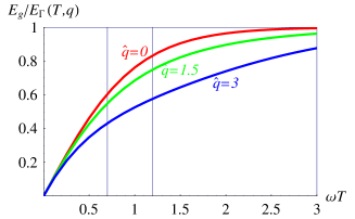
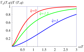
(a)	(b)

Fig. 1: Relative ground-state contribution to (a) the energy $E_{\Gamma}(T,q)$ and (b) the correlator $\Gamma(T,q)$ vs. $T$ for several values of $q$. The vertical lines indicate the boundaries of the “Borel window”.

Let us now construct for $\Gamma(T,q)$ the analogue of the OPE as used in the method of three-point sum rules in QCD. First, we expand $\Gamma$ in powers of $\omega^{2}$ and obtain

$$\Gamma(T,q)=\sum\limits_{n=0}^{\infty}\Gamma_{2n}(T,q)\omega^{2n}.$$ (2.20)

This expansion is the analogue of the expansion of the vertex function in terms of the nonlocal condensates in QCD nonlocal . Explicitly, for the lowest terms one has

$$\Gamma_{0}(T,q) = \left(\frac{m}{2\pi T}\right)^{3/2}\exp\left(-\frac{q^{2}T}{8m}\right),$$

$$\Gamma_{2}(T,q) = \left(\frac{m}{2\pi T}\right)^{3/2}\exp\left(-\frac{q^{2}T}{8m}\right)\left(-\frac{1}{4}+\frac{q^{2}T}{96m}\right)\omega^{2}T^{2},\quad\ldots.$$ (2.21)

The first term, $\Gamma_{0}$, corresponds to free propagation and does not depend on the confining potential. It may be written as the double spectral representation lms_prd75

$$\Gamma_{0}(T,q) = \int_{0}^{\infty}dz_{1}dz_{2}e^{-{\frac{1}{2}}z_{1}T}e^{-{\frac{1}{2}}z_{2}T}\Delta_{0}(z_{1},z_{2},q),$$ (2.22)

$$\Delta_{0}(z_{1},z_{2},q) = \frac{m^{2}}{4\pi^{2}q}\theta\left(\left(z_{1}+z_{2}-\frac{q^{2}}{2m}\right)^{2}-4z_{1}z_{2}<0\right).$$

The Ward identity in nonrelativistic field theory relates to each other the three-point function at zero momentum transfer and the two-point function and leads to

$$\lim_{q\to 0}\Delta_{0}(z,z^{\prime},q)=\delta(z-z^{\prime})\rho_{0}(z).$$ (2.23)

Power corrections are defined as the difference between the exact expression and the free diagram:

$$\Gamma_{\rm OPE}(T,q)=\Gamma_{0}(T,q)+\Gamma_{\rm power}(T,q).$$ (2.24)

In order to obtain the analogue of the OPE for $\Gamma$ in terms of local condensates, one should further expand $\Gamma_{\rm power}(T,q)$ (i.e., $\Gamma_{2n}(T,q),$ $n\geq 1$) in powers of $T$.

2.3 Vacuum-to-hadron correlator

In order to apply the method of sum rules to hadron form factors at intermediate and large momentum transfers a Borelized vacuum-to-hadron amplitude of the $T$-product of two quark currents is used stern . The analogue of this quantity in quantum mechanics has the form m_lcsr

$$A(T,q)=\langle{{\bf r}=0}|G(T)J({\bf q})|\psi_{\rm g}\rangle,\qquad G(T)\equiv\exp(-HT).$$ (2.25)

The spectral representation for $A(T,q)$ may be written in the form

$$A(T,q)=\int d^{3}k\;G(k^{2},T)\psi_{\rm g}({\bf k}-{\bf q})=\int_{0}^{\infty}dz\,\exp(-zT)\rho_{A}(z,T,q),\quad z\equiv{k}^{2}/2m,$$ (2.26)

where nsvz

$$G(k^{2},T)\equiv\langle{{\bf r}=0}|G(T)|{\bf k}\rangle=\frac{1}{(2\pi)^{3/2}}\frac{1}{[\cosh(\omega T)]^{3/2}}\exp\left(-\frac{k^{2}}{2m\omega}\tanh(\omega T)\right).$$ (2.27)

Explicit expressions for $\rho_{A}(z,T,q)$ and $A(T,q)$ may be obtained using $\psi_{\rm g}$ of Eq. (2.2); for instance, for $A(T,q)$ one finds

$$A(T,q)=\sqrt{R_{\rm g}}\exp\left({-E_{\rm g}T}\right)\exp\left(-\frac{q^{2}}{4m\omega}\left(1-e^{-2\omega T}\right)\right).$$ (2.28)

The function $A(T,q)$ depends on two dimensionless variables ${\hat{q}}^{2}={q^{2}}/{m\omega}$ and $\omega T$.

Expanding in Eq. (2.26) the Green function $G(k^{2},T)$ in powers of $\omega$ generates the analogue of the QCD twist expansion for the amplitude $A(T,q)$ (see m_lcsr for details).

The ground-state contribution to the correlator has the form

$$A_{\rm g}(T,q)=\sqrt{R_{\rm g}}\exp\left({-E_{\rm g}T}\right)F_{\rm g}(q),$$ (2.29)

so one finds

$$\frac{A_{\rm g}(T,q)}{A(T,q)}=\exp\left(-\frac{q^{2}}{4m\omega}e^{-2\omega T}\right).$$ (2.30)

Notice the following features of the correlator $A(T,q)$ (see Fig. 2):

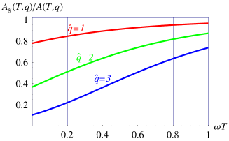
(a)	(b)

Fig. 2: Relative ground-state contribution to (a) the energy $E_{A}(T,q)$ and (b) the correlator $A(T,q)$ vs. $T$ for several values of $q$. The vertical lines indicate the boundaries of the “Borel window”.

(i) At large $T$, the ground state provides the dominant contribution to $A$, similar to the case of vacuum-to-vacuum correlators:

$$A(T,q)\to A_{\rm g}(T,q)\quad\mbox{for}\quad T\to\infty.$$ (2.31)

(ii) At small $q$, because of current conservation, the ground state dominates the correlator for all $T$. This is a specific feature of $A$ which arises due to the choice of the initial state. Thus, compared with vacuum-to-vacuum correlators, the correlator $A$ “maximizes” the ground-state contribution.

2.4 Dual correlators and effective continuum thresholds

The sum rule for each of the correlators described above is an expression of the fact that the correlator calculated in terms of the constituent degrees of freedom (quarks and gluons) and the bound-state degrees of freedom (hadrons) are equal to each other. In order to isolate the ground-state contributions from the sums over hadron spectra, one invokes quark-hadron duality which assumes that the excited states are dual to the high-energy regions — i.e., the regions above some effective continuum thresholds — of the spectral representations for the correlators. The correlators to which the corresponding cuts have been applied are referred to as the dual correlators. The relations between the ground-state contributions and the dual correlators take the following form:

$$R_{\rm g}e^{-{E_{\rm g}}T} = \Pi_{\rm dual}(T,z^{\Pi}_{\rm eff}(T))\equiv\int\limits_{0}^{z^{\Pi}_{\rm eff}(T)}dz\,e^{-zT}\rho_{0}(z)+\Pi_{\rm power}(T),$$ (2.32)

$$F_{\rm g}(q)R_{\rm g}e^{-{E_{\rm g}}T} = \Gamma_{\rm dual}(T,q,z^{\Gamma}_{\rm eff}(T,q))\equiv\int\limits_{0}^{z^{\Gamma}_{\rm eff}(T,q)}dz_{1}\int\limits_{0}^{z^{\Gamma}_{\rm eff}(T,q)}dz_{2}\,e^{-\frac{1}{2}(z_{1}+z_{2})T}\Delta_{0}(z_{1},z_{2},q)+\Gamma_{\rm power}(T,q),$$ (2.33)

$$F_{\rm g}(q)\sqrt{R_{\rm g}}e^{-{E_{\rm g}}T} = A_{\rm dual}(T,q,z^{A}_{\rm eff}(T,q))\equiv\int_{0}^{z^{A}_{\rm eff}(T,q)}dz\,e^{-zT}\rho_{A}(z,T,q).$$ (2.34)

As consequence of (2.15), $\Pi_{\rm power}(T)=\Gamma_{\rm power}(T,q=0)$ and

$$z^{\Pi}_{\rm eff}(T)=z^{\Gamma}_{\rm eff}(T,q=0).$$ (2.35)

Then, due to the Ward identity (2.23), the relations (2.32) and (2.33) yield the correct normalization of the form factor $F_{\rm g}(q=0)=1$, as required by current conservation.

Let us take advantage of knowing the exact ground-state parameters in the potential model and calculate the exact effective continuum thresholds for all the correlators. These exact thresholds are obtained by solving the equations above for the exact ground-state parameters on the l.h.s.; the exact thresholds make the quark-hadron duality relations (2.32)–(2.34) exact. Clearly, $z^{\Gamma}_{\rm exact}(T,q=0)=z^{\Pi}_{\rm exact}(T)$. Figure 3 depicts the exact effective continuum thresholds for $\Gamma(T,q)$ and $A(T,q)$.

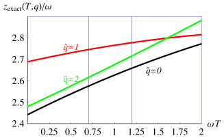
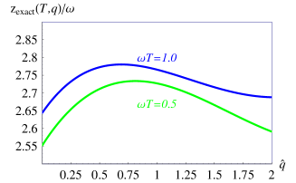
(a)	(b)
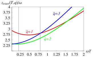
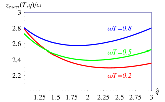
(c)	(d)

Fig. 3: Exact effective continuum threshold $z^{\Gamma}_{\rm exact}(T,q)$ (a,b) and $z^{A}_{\rm exact}(T,q)$ (c,d). $z^{\Pi}_{\rm exact}(T)=z^{\Gamma}_{\rm exact}(T,q=0)$. The vertical lines indicate the “Borel window”.

As is obvious from Fig. 3, the effective continuum thresholds do depend considerably on both $T$ and $q$. Moreover, for the same theory (i.e., the same potential and the same values of its parameters) the exact effective thresholds for $\Gamma(T,q)$ and $A(T,q)$ are rather different from each other and have very different $T$- and $q$-dependencies.

It might be useful to notice that the dependence of the effective thresholds on the Borel parameter, being unusual for spectral representations, does not contradict any properties of field theory: the dual correlators are hand-made objects and they cannot be written as, e.g., the $T$-product of local currents; thus the dual correlators have completely different analytic properties than the “usual” correlators in field theory.

To summarize, the exact effective continuum thresholds (i) depend on $T$ and on $q$; (ii) are not “universal”, i.e., for one and the same ground state, the effective thresholds in different correlators strongly differ from each other. As a consequence, making use of the effective continuum threshold obtained, e.g., for $\Pi_{\rm dual}$ as effective thresholds for the dual correlators $\Gamma_{\rm dual}$ or $A_{\rm dual}$, as often done in practical applications of the sum-rule method in QCD, has no ground and may lead to very inaccurate estimates for the form factors.

On the practical side, a good or a bad extraction of the ground-state parameters depends on our capacity to find a reasonable approximation to the exact effective continuum threshold.

2.5 Numerical analysis

Let us consider a restricted problem where the energy $E_{\rm g}$ of the ground state and its wave function at the origin, $\sqrt{R_{\rm g}}$, are known, and try to extract its elastic form factor from the sum rules (2.33) and (2.34).

A. First, according to svz we should determine the working interval of $T$ — the “Borel window” — where the method may be applied to the extraction of the ground-state parameter:

(i) The upper boundary of the $T$-window is obtained from the condition that the truncated expansion gives a good approximation to the exact correlator. Since in the HO model the correlators are known exactly, the upper boundary is $T=\infty$. However, to be close to realistic situations, where only a limited number of higher-order or higher-twist corrections is available, following our results reported in lms_3ptsr ; m_lcsr we define the upper boundary of the window as $\omega T\lesssim 1.2$ for $\Gamma(T,q)$ and $\omega T\lesssim 0.8$ for $A(T,q)$.

(ii) The lower boundary of this $T$-window is determined by the condition that the ground state gives a “sizable” contribution to the correlator. If we require the ground-state contribution to exceed, say, 50%, the window for $\Gamma(T,q)$ closes already for $\hat{q}\simeq 2$ (Fig. 1b), whereas for $A(T,q)$ it closes for $\hat{q}\simeq 4$ (Fig. 2b).

We shall see, however, that our algorithm will allow us to extract the form factor, although with a worse accuracy, also in the region where the ground-state contribution to the correlator remains well below 50%. Thus, our algorithm opens the possibility to study also the region of larger momentum transfers.

We choose the “windows” as follows:

$$0.7\lesssim\omega T\lesssim 1.2\quad\mbox{ for }\Gamma(T,q),$$ (2.36)

$$0.2\lesssim\omega T\lesssim 0.8\quad\mbox{ for }A(T,q).$$ (2.37)

B. Second, we must choose a criterion to fix the effective continuum threshold $z_{\rm eff}(T,q)$. We proceed in the following way: We consider a set of $T$-dependent Ansätze for the effective continuum threshold

$$z^{(n)}_{\rm eff}(T,q)=\sum\limits_{j=0}^{n}z_{j}^{(n)}(q)(\omega T)^{j}.$$ (2.38)

(The standard procedure adopted in all sum-rule applications in QCD is to assume a $T$-independent quantity. Obviously, this option is also included in our analysis.) Now, at each value of $q$ we fix the parameters on the r.h.s of (2.38) as follows: we calculate the dual energy

$$E^{\Gamma}_{\rm dual}(T,q) = -\frac{d}{dT}\log\Gamma_{\rm dual}(T,q,z^{\Gamma}_{\rm eff}(T,q)),$$ (2.39)

$$E^{A}_{\rm dual}(T,q) = -\frac{d}{dT}\log A_{\rm dual}(T,q,z^{A}_{\rm eff}(T,q)),$$ (2.40)

for the $T$-dependent $z_{\rm eff}$ of Eq. (2.38). Then we evaluate $E_{\rm dual}(T,q)$ at several values of $T=T_{i}$ ($i=1,\dots,N$, where $N$ can be taken arbitrarily large) chosen uniformly in the window. Finally, we minimize the squared difference between $E_{\rm dual}$ and the exact value $E_{\rm g}$:

$$\chi^{2}\equiv\frac{1}{N}\sum_{i=1}^{N}\left[E^{(A,\Gamma)}_{\rm dual}(T_{i},q)-E_{\rm g}\right]^{2}.$$ (2.41)

Recall that the exact effective continuum thresholds for the two correlators $\Gamma(T,q)$ and $A(T,q)$ have rather different $T$-dependencies, see Fig. 3. Therefore, one should expect that the expressions (2.38) for the corresponding effective thresholds will be different.

The results for the form factor obtained from $\Gamma(T,q)$ and from $A(T,q)$ upon optimizing the parameters of $z^{\Gamma}_{\rm eff}$ and $z^{A}_{\rm eff}$ according to (2.41) are shown in Fig. 4.

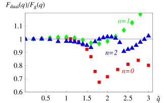
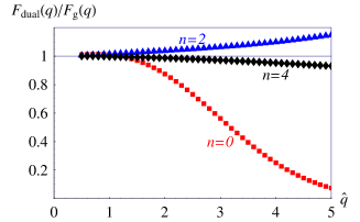
(a)	(b)

Fig. 4: The dual form factor $F_{\rm dual}(q)$ extracted from (a) the correlator $\Gamma(T,q)$ and (b) the correlator $A(T,q)$. Red symbols ($n=0$) correspond to the standard $T$-independent Ansatz for $z_{\rm eff}$, green ($n=1$) to the linear Ansatz, blue ($n=2$) to the quadratic Ansatz, and black ($n=4$) to the quartic Ansatz.

2.5.1 Form factor from $\Gamma(T,q)$

Let us first consider the extraction of the form factor from the correlator $\Gamma(T,q)$.

Within the standard $T$-independent approximation, one extracts the form factor in the region $\hat{q}\leq 1.5$ with better than 10% accuracy, while the accuracy decreases rather fast for higher $q$ (see Fig. 4a). The dramatic increase of the error at $\hat{q}\gtrsim 2$ is related to the fact that the contribution of the ground state to the correlator decreases rapidly with $q$ in the given $T$-window $0.7\leq\omega T\leq 1.2$ (see Fig. 1).

The real problem is, however, that the magnitude of the error cannot be obtained on the basis of the standard criteria adopted in the method: e.g., at $\hat{q}=2$, the variation of the extracted form factor in the window is only about 2% (see Fig. 5b) which mimics an accurate extraction of the form factor, whereas the actual error comprises 25%. Thus, within a $T$-independent Ansatz for the effective threshold, the error of the form factor cannot be determined from the variation of the dual form factor in the window.

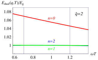
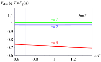
(a)	(b)

Fig. 5: The correlator $\Gamma(T,q)$: the fitted dual energy $E_{\rm dual}(T,q)$ and the corresponding dual form factor $F_{\rm dual}(T,q)$ for $\hat{q}=2$. Red lines ($n=0$) correspond to the standard $T$-independent Ansatz for $z_{\rm eff}$, green lines ($n=1$) to the linear Ansatz, and blue lines ($n=2$) to the quadratic Ansatz.

Allowing for the $T$-dependent effective threshold leads to a considerable improvement of the accuracy: both for the linear and the quadratic Ansätze for the threshold, the dual energy reproduces the known energy rather accurately in the window, and the dual form factor reproduces the exact form factor rather well. Noteworthy, the actual error of the extracted form factor may be obtained as the spread between the dual form factors obtained for the linear and the quadratic Ansätze for $z_{\rm eff}$.

2.5.2 Form factor from $A(T,q)$

Let us now consider the extraction of the form factor from the correlator $A(T,q)$.

The standard $T$-independent Ansatz works well below $\hat{q}\leq 1.5-2$, but for larger $\hat{q}$ the accuracy of the extracted form factor decreases very fast, see Fig. 4. The main problem here is the same as for the case of $\Gamma(T,q)$: the large error in the extracted form factor cannot be guessed on the basis of the standard Borel stability criterion: as seen in Fig. 6, the variation of the form factor at $\hat{q}=2$ in the window comprises only 2%, whereas the actual error exceeds 10%.

Allowing for $T$-dependent approximations for $z_{\rm eff}$ leads to considerable improvements: as shown in Fig. 4, the form factor may be extracted with a reasonable accuracy (better than 15%) up to $\hat{q}=5$ with the quadratic and quartic Ansätze, $z^{(2)}_{\rm eff}(T,q)$ and $z^{(4)}_{\rm eff}(T,q)$ (the results obtained for $n=1$ are close to the results for $n=0$, and the results for $n=3$ are close to those for $n=2$).

This high accuracy is achieved in spite of the fact that (i) the relative contribution of the ground state to the correlator falls down considerably below 50% in the $T$-window, and (ii) the form factor at $\hat{q}=5$ falls down compared to its value at $\hat{q}=0$ by almost three orders of magnitude.

Notice again the typical feature of the extraction procedure: both for $n=2$ and $n=4$ both the dual energy $E_{\rm dual}(T,q)$ and the dual form factor $F_{\rm dual}(T,q)$ are extremely stable (better than $0.1\%$) in the window for all $\hat{q}\leq 5$ (Fig. 6 shows the results for $\hat{q}=2$). In spite of this stability, the actual error of the extracted form factor for $n=2$ and $n=4$, separately, is found to be much larger: e.g., at $\hat{q}=5$ this error comprises 10–15%. Again, this error could not be guessed on the basis of the standard Borel stability criterion, which thus does not work also for vacuum-to-hadron correlators.

Nevertheless, we have seen clear improvements in the results of the extraction procedure as soon as one goes beyond the assumption of a $T$-independent effective continuum threshold: First, the actual accuracy turns out to be (much) better. Second, the $T$-dependent Ansatz allows one to extract the form factor in a broader range of the momentum transfer. Finally, the spread between the results obtained with the quadratic and the quartic Ansätze for $z_{\rm eff}$ provides the actual error of the extracted form factor.

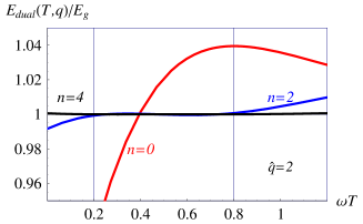
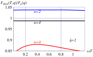
Fig. 6: The correlator $A(T,q)$: the fitted dual energy $E_{\rm dual}(T,q)$ and the corresponding dual form factor $F_{\rm dual}(T,q)$ for $\hat{q}=2$. Red lines ($n=0$) correspond to the standard $T$-independent Ansatz for $z_{\rm eff}$, blue lines ($n=2$) to the quadratic Ansatz; and black lines ($n=4$) to the quartic Ansatz.

3 Potential model vs. QCD

In the previous section we have shown that the concept of the $T$-dependent effective continuum threshold and the way of fixing this quantity by reproducing the bound-state energy has led to a dramatic increase of the actual accuracy of the extracted form factor in the potential model.

Does this new approach to the extraction of the properties of ground-state hadrons promise equivalent improvements in QCD? We give a positive answer to this question lms_qmvsqcd .

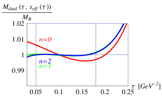
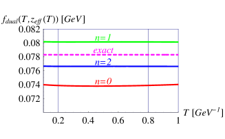
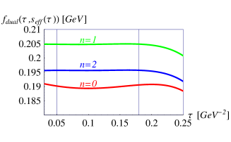
Fig. 7: Dual mass and extracted dual decay constant vs. Borel parameter in the potential model (left column) and in QCD (right column). In QCD, the Borel parameter $\tau$ has dimension $GeV^{-2}$.

Figure 7 compares the extraction of the ground-state decay constant from the two-point function in the potential model (left column) and in QCD (right column). For the potential model, we consider the interaction consisting of a confining HO part and a Coulomb part and make use of the OPE which includes the radiative corrections up to order $\alpha^{2}$ and several lowest-order power corrections. This corresponds to the best known OPE for the two-point function of heavy-light quark currents jamin which we use for QCD. Details of this analysis including the specific values of the numerical parameters can be found in lms_qmvsqcd ; they are not essential for our purpose here.

From Fig. 7 it becomes evident that — with respect to the extraction of the ground-state parameters — there are no essential differences between QCD and quantum mechanics: as soon as the parameters of the Lagrangian are fixed, and the truncated OPE is calculated with a reasonable accuracy (taking into account also the relevant choice of the renormalization scale in QCD), the extraction procedures are very similar.

At first glance, this similarity might look surprising since the structure of bound states in quantum-mechanical potential models and in QCD are rather different. However, the method of dispersive sum rules does not make use of the details of the ground-state structure. What really matters for extracting the ground-state parameters by this method is (i) the way one implements the quark-hadron duality and (ii) the structure of the OPE for a given correlator. Therefore, it should not be surprising that the extraction procedures in potential models and in QCD are similar, as soon as quark-hadron duality is implemented in both theories in the same way by a cut on the spectral representation for the correlators.

In the potential model, the actual value of the decay constant belongs to the band provided by the linear and the quadratic Ansätze for the effective continuum threshold. It seems very likely that the same happens in QCD, at least this may be taken as a realistic conjecture. Perhaps even more important is that studying the $\tau$-dependent parameterizations for the effective threshold allows one to probe the magnitude of the intrinsic, i.e., systematic, uncertainty of the extracted decay constant. Interestingly, the systematic uncertainties of the ground-state parameters are probed solely by the OPE, without making use of the information about the excited states of the hadron spectrum. The intrinsic uncertainty should be taken into account along with the “usual” uncertainty obtained in the method of QCD sum rules by the variation of the input QCD parameters; while the latter is going to decrease when increasing the accuracy of these parameters, e.g., $m_{b}(m_{b})$, the systematic uncertainty does not depend on the input QCD parameters and remains at the same level.

4 Conclusions

We studied the extraction of the ground-state form factor from the vacuum-to-vacuum and vacuum-to-hadron correlators. Let us summarize the main messages of our analysis:

• The knowledge of the correlator in a limited range of relatively small Euclidean times $T$ (i.e., large Borel masses) is not sufficient for the determination of the ground-state parameters. In addition to the OPE for the relevant correlator, one needs an independent criterion for fixing the effective continuum threshold.

• Assuming a $T$-independent (i.e., a Borel-parameter-independent) effective continuum threshold, the error of the extracted dual form factor $F_{\rm dual}(T,q)$ turns out to be typically much larger than the variation of $F(T,q)$ in the Borel window. Therefore the standard procedures based on the Borel stability adopted in the method of sum rules do not allow one to obtain realistic error estimates for the extracted form factor; eventually the actual error of the extracted form factor may happen to be much larger.

• In those cases where the ground-state energy (mass) is known, considerable improvements may be achieved by allowing for a $T$-dependent effective continuum threshold and finding its parameters by minimizing the deviation of the energy of the dual correlator from the known value of the ground-state energy, Eq. (2.41). First, the actual accuracy of the extracted form factor is considerably improved. Second, the spread between form-factor values obtained with different $T$-dependent Ansätze for $z_{\rm eff}$ provides a realistic error of the form factor.

• We have demonstrated the striking similarity — not only qualitatively but, more importantly, also quantitatively — between the extraction procedures in the quantum-mechanical potential model and in QCD. This similarity is the consequence of the same way of implementing the quark-hadron duality in both theories. The established similarity strongly suggests that the results on the extraction of ground-state form factors obtained in potential models have direct implications for the corresponding analyses in QCD and should be taken very seriously.

  Although a rigorous — in the mathematical sense — control over the systematic errors of the extracted hadron parameters remains unfeasible, the proposed modifications related to the Borel-parameter-dependent effective continuum threshold promise a considerable increase of the actual accuracy of the method of sum rules and opens the possibility to obtain realistic estimates for the systematic errors.

Acknowledgments. We are grateful to Hagop Sazdjian for the most pleasant collaboration on several issues discussed in this paper. D. M. gratefully acknowledges financial support from the Austrian Science Fund (FWF) under project P20573 and from the President of Russian Federation under grant for leading scientific schools 1456.2008.2.

References

- (1) M. Shifman, A. Vainshtein, and V. Zakharov, Nucl. Phys. B 147, 385 (1979).
- (2) B. L. Ioffe and A. V. Smilga, Phys. Lett. B 114, 353 (1982); V. A. Nesterenko and A. V. Radyushkin, Phys. Lett. B 115, 410 (1982).
- (3) V. M. Belyaev et al., Phys. Rev. D 51, 6177 (1995).
- (4) S. Ahmed et al. (CLEO Collaboration), Phys. Rev. Lett. 87, 251801 (2001).
- (5) V. M. Braun, A. Khodjamirian, and M. Maul, Phys. Rev. D 61, 073004 (2000).
- (6) V. Braguta, W. Lucha, and D. Melikhov, Phys. Lett. B 661, 354 (2008).
- (7) A. P. Bakulev, A. V. Pimikov, and N. G. Stefanis, Phys. Rev. D 79, 093010 (2009).
- (8) A. I. Vainshtein, V. I. Zakharov, V. A. Novikov, and M. A. Shifman, Sov. J. Nucl. Phys. 32, 840 (1980).
- (9) V. Novikov, M. Shifman, A. Vainshtein, and V. Zakharov, Nucl. Phys. B 237, 525 (1984).
- (10) V. A. Novikov et al., Phys. Rep. 41, 1 (1978); M. B. Voloshin, Nucl. Phys. B 154, 365 (1979); J. S. Bell and R. Bertlmann, Nucl. Phys. B 177, 218 (1981); 187, 285 (1981); V. A. Novikov, M. A. Shifman, A. I. Vainshtein, and V. I. Zakharov, Nucl. Phys. B 191, 301 (1981).
- (11) A. Le Yaouanc et al., Phys. Rev. D 62, 074007 (2000); Phys. Lett. B 488, 153 (2000); Phys. Lett. B 517, 135 (2001).
- (12) D. Melikhov and S. Simula, Phys. Rev. D 62, 074012 (2000).
- (13) A. V. Radyushkin, in Strong Interactions at Low and Intermediate Energies, ed. by J. L. Goity, (World Sci., Singapore), p. 91, 2000, hep-ph/0101227.
- (14) W. Lucha, D. Melikhov, and S. Simula, Phys. Rev. D 76, 036002 (2007); Phys. Lett. B 657, 148 (2007); Phys. At. Nucl. 71, 1461 (2008).
- (15) W. Lucha, D. Melikhov, and S. Simula, Phys. Lett. B 671, 445 (2009).
- (16) D. Melikhov, Phys. Lett. B 671, 450 (2009).
- (17) W. Lucha, D. Melikhov, and S. Simula, Phys. Rev. D 79, 096011 (2009).
- (18) W. Lucha, D. Melikhov, and S. Simula, J. Phys. G 37, 035003 (2010).
- (19) W. Lucha, D. Melikhov, H. Sazdjian, and S. Simula, Phys. Rev. D 80, 114028 (2009).
- (20) N. S. Craigie and J. Stern, Nucl. Phys. B 216, 209 (1983).
- (21) A. P. Bakulev and A. V. Radyushkin, Phys. Lett. B 271, 223 (1991).
- (22) D. Melikhov, Eur. Phys. J. direct C 4, 2 (2002), hep-ph/0110087; D. Melikhov and S. Simula, Eur. Phys. J. C 37, 437 (2004); W. Lucha, D. Melikhov, and S. Simula, Phys. Rev. D 75, 016001 (2007).
- (23) W. Lucha, D. Melikhov, and S. Simula, arXiv:0912.5017, Phys. Lett. B (in print).
- (24) M. Jamin and B. Lange, Phys. Rev. D 65, 056005 (2002).