Radiative hydrodynamics simulations of red supergiant stars: II. simulations of convection on Betelgeuse match interferometric observations

Abstract

Context. The red supergiant (RSG) Betelgeuse is an irregular variable star. Convection may play an important role in understanding this variability. Interferometric observations can be interpreted using sophisticated simulations of stellar convection.

Aims. We compare the visibility curves and closure phases obtained from our 3D simulation of RSG convection with CO5BOLD to various interferometric observations of Betelgeuse from the optical to the H band in order to characterize and measure the convection pattern on this star.

Methods. We use 3D radiative-hydrodynamics (RHD) simulation to compute intensity maps in different filters and we thus derive interferometric observables using the post-processing radiative transfer code OPTIM3D. The synthetic visibility curves and closure phases are compared to observations.

Results. We provide a robust detection of the granulation pattern on the surface of Betelgeuse in the optical and in the H band based on excellent fits to the observed visibility points and closure phases. Moreover, we determine that the Betelgeuse surface in the H band is covered by small to medium scale (5–15 mas) convection-related surface structures and a large ($\approx$30 mas) convective cell. In this spectral region, H₂O molecules are the main absorbers and contribute to the small structures and to the position of the first null of the visibility curve (i.e. the apparent stellar radius).

1 Introduction

Betelgeuse is a red supergiant star (Betelgeuse, HD 39801, M1–2Ia–Ibe) and is one of the brightest stars in the optical and near infrared. This star exhibits variations in integrated brightness, surface features, and the depths, shapes, and Doppler shifts of its spectral lines. There is a backlog of visual-wavelength observations of its brightness which covers almost a hundred years. The irregular fluctuations of its light curve are clearly aperiodic and rather resemble a series of outbursts. Kiss et al. (2006) studied the variability of different red supergiant (RSG) stars including Betelgeuse and they found a strong noise component in the photometric variability, probably caused by the large convection cells. In addition to this, the spectral line variations have been analyzed by several authors, who inferred the presence of large granules and high convective velocities (Josselin & Plez, 2007; Gray, 2008). Gray also found line bisectors that predominantly have reversed C-shapes, and line shape variations occurring at the 1 km s^-1 level that have no obvious connection to their shifts in wavelength.

The position of Betelgeuse on the H-R diagram is highly uncertain, due to uncertainty in its effective temperature. Levesque et al. (2005) used one-dimensional MARCS models (Gustafsson et al., 2003, 1975) to fit the incredibly rich TiO molecular bands in the optical region of the spectrum for several RSGs. They found an effective temperature of 3650 K for Betelgeuse. Despite the fact that they obtained a good agreement with the evolutionary tracks, problems remain. There is a mismatch in the IR colors that could be due to atmospheric temperature inhomogeneities characteristic of convection (Levesque et al., 2006). Also the distance of Betelgeuse has large uncertainities because of errors related to the positional movement of the stellar photocenter. Harper et al. (2008) derived a distance of (197$\pm$45 pc) using high spatial resolution, multiwavelength, VLA radio positions combined with Hipparcos Catalogue Intermediate Astrometric Data.

Betelgeuse is one of the best studied RSGs in term of multi-wavelength imaging because of its large luminosity and angular diameter. The existence of hot spots on its surface has been proposed to explain numerous interferometric observations with WHT and COAST (Buscher et al., 1990; Wilson et al., 1992; Tuthill et al., 1997; Wilson et al., 1997; Young et al., 2000, 2004) that have detected time-variable inhomogeneities in the brightness distribution. These authors fitted the visibility and closure phase data with a circular limb-darkened disk and zero to three spots. A large spot has been also detected by Uitenbroek et al. (1998) with HST. The non-spherical shape of Betelgeuse was also detected by Tatebe et al. (2007) in the mid-infrared. Haubois et al. (2009) published a reconstructed image of Betelgeuse in the H band with two spots using the same data as presented in this work. Kervella et al. (2009) resolved Betelgeuse using diffraction-limited adaptive optics in the near-infrared and found an asymmetric envelope around the star with a bright plume extending in the southwestern region. They claimed the plume was either due to the presence of a convective hot spot or was caused by stellar rotation. Ohnaka et al. (2009) presented VLTI/AMBER observations of Betelgeuse at high spectral resolution and spatially resolved CO gas motions. They claimed that these motions were related to convective motions in the upper atmosphere or to intermittent mass ejections in clumps or arcs.

Radiation hydrodynamics (RHD) simulations of red supergiant stars are available (Freytag et al., 2002) to interpret past and future observations. (Chiavassa et al., 2009, hereafter Paper I) used these simulations to explore the impact of the granulation pattern on observed visibility curves and closure phases and detected a granulation pattern on Betelgeuse in the K band by fitting the existing interferometric data of Perrin et al. (2004).

This paper is the second in the series aimed at exploring the convection in RSGs. The main purpose is to compare RHD simulations to high-angular resolution observations of Betelgeuse covering a wide spectral range from the optical region to the near-infrared H band, in order to confirm the presence of convective cells on its surface.

2 3D radiation-hydrodynamics simulations and post-processing radiative transfer

We employed numerical simulations obtained using CO⁵BOLD (Freytag et al., 2002; Freytag, 2003; Freytag & Höfner, 2008) and in particular the model st35gm03n07 that has been deeply analyzed in Paper I. The model has 12 $M_{\odot}$, a numerical resolution of 235³ grid points with a step of 8.6 $R_{\odot}$, an average luminosity over spherical shells and over time of $L$=93000$\pm$1300 $L_{\odot}$, an effective temperature of $T_{\rm{eff}}$=3490$\pm$13 K, a radius of $R$=832$\pm$0.7 $R_{\odot}$, and surface gravity log($g$)=-0.337$\pm$0.001. This is our “best” RHD simulation so far because it has stellar parameters closest to Betelgeuse ($T_{\rm{eff}}=3640$ K, Levesque et al., 2005; and log($g$)=-0.3, Harper et al., 2008).

We used the 3D pure-LTE radiative transfer code OPTIM3D described in Paper I to compute intensity maps from all the suitable snapshots of the 3D hydrodynamical simulation. The code takes into account the Doppler shifts caused by the convective motions. The radiation transfer is calculated in detail using pre-tabulated extinction coefficients generated with the MARCS code (Gustafsson et al., 2008). These tables are functions of temperature, density and wavelength, and were computed with the solar composition of Asplund et al. (2006). The tables include the same extensive atomic and molecular data as the MARCS models. They were constructed with no micro-turbulence broadening and the temperature and density distributions are optimized to cover the values encountered in the outer layers of the RHD simulations.

3 Observations

The data presented in this work have been taken by two independent groups with different telescopes and they cover a large wavelength range from the optical to the near infrared. The log of the observations is reported in Table 1

Table 1: Log of the observations.

Date	Telescope	Filter (central $\lambda$)
October 7, 2005	IOTA	IONIC - 16000
October 8, 2005	IOTA	IONIC - 16000
October 10, 2005	IOTA	IONIC - 16000
October 11, 2005	IOTA	IONIC - 16000
October 12, 2005	IOTA	IONIC - 16000
October 16, 2005	IOTA	IONIC - 16000
October 21, 1997	COAST	12900 Å
October 24, 1997	COAST	9050 Å
October 31, 1997	COAST	9050 Å
November 11, 1997	COAST	12900 Å
November 12, 1997	COAST	9050 Å
November 15, 1997	WHT	7000 Å
November 16, 1997	WHT	9050 Å
November 21, 1997	COAST	9050 Å
January 29, 2004	COAST	7500, 7820, 9050 Å
February 8, 2004	COAST	7500, 7820, 9050 Å
February 25, 2004	COAST	7500, 7820, 9050 Å
February 29, 2004	COAST	7500, 7820, 9050 Å
March 1, 2004	COAST	7500, 7820, 9050 Å
March 2, 2004	COAST	7500, 7820, 9050 Å

3.1 Data at 16400 Å.

The H band data were acquired with the 3 telescope interferometer IOTA (Infrared Optical Telescope Array, Traub et al., 2003) located at Mount Hopkins in Arizona. Light collected by three apertures (siderostats of 0.45m diameter) was spatially filtered by single mode fibers to clean the wavefronts, removing high frequency atmospheric corrugations that affect the fringe contrast. The beams were then combined with IONIC (Berger et al., 2003). This integrated optics component combines 3 input beams in a pairwise manner. Fringes were encoded in the time domain using piezo-electric path modulators, and detected with a near-infrared camera utilizing a PICNIC detector (Pedretti et al., 2004).

Betelgeuse was observed in the H band ($16400\pm 1000$ Å, Fig. 1) on 6 nights between 7th October and 16th October 2005. Five different configurations of the interferometer telescopes were used, in order to cover a large range of spatial frequencies between 12 and 95 arcsec^-1. To calibrate the instrumental transfer function, observations of Betelgeuse were interleaved with observations of a reference (calibrator) star, HD 36167.

Data reduction was carried out using an IDL pipeline (Monnier et al., 2004; Zhao et al., 2007). In order to measure the closure phase, we took the phase of the complex triple product (bispectrum, Baldwin et al., 1986). The instrumental closure phase of IONIC3 drifted less than 1 degree over many hours owing to the miniature dimensions of the integrated optics component. Both for the squared visibilities and the closure phase, the random errors were calculated with the bootstrap technique, in which a statistic is repeatedly re-estimated by Monte-Carlo sampling the original data with replacement. Full details of the observations and data reduction can be found in Haubois et al. (2009).

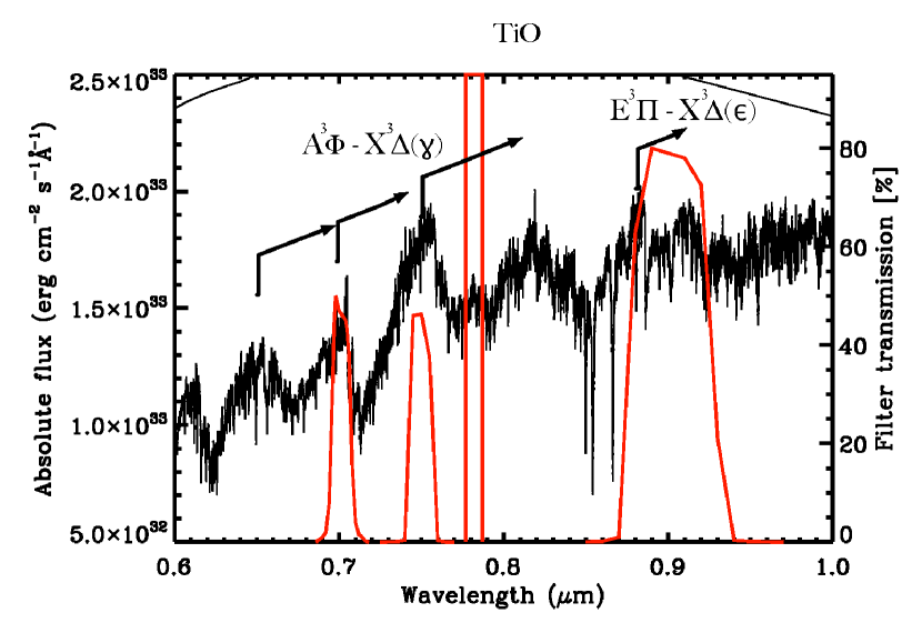
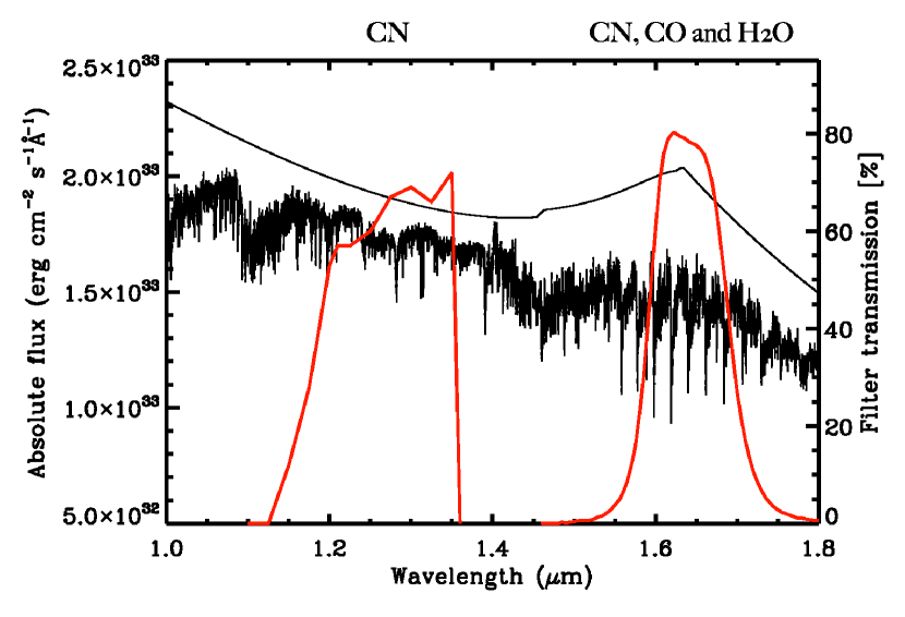
Figure 1: Transmission curves (red) of the bandpass filters used for Betelgeuse observations at COAST and WHT: central wavelengths at 7000, 7500, 7820, 12900 Å and nominal bandwidths (FWHM) of 100, 130, 50, 500, 1500 Å respectively (Young et al., 2004, 2000) (the filter curve for the narrow bandpass centered at 7820 Å has been lost hence we assumed a top-hat filter); and for Betelgeuse observations at IOTA: 16400 Å with 1000 Å bandwidth (Haubois et al., 2009). The black line is the synthetic spectrum with its continuum computed from the RHD simulation snapshot of Fig. 8; the molecules that contribute the most in every filter have been highlighted.

3.2 Data from 7000 to 12900 Å.

For this wavelength range, we used data taken at two different epochs. The observations carried out in 1997 (Young et al., 2000) were acquired with the Cambridge Optical Aperture Synthesis Telescope (COAST) on baselines up to 8.9 m (with central wavelengths/bandwidths of 9050/500 and 12900/1500 Å) and by non-redundant aperture masking with the William Herschel Telescope (WHT) on baselines up to 3.7 m (with central wavelengths/bandwidths of 7000/100 and 9050/500). The observations carried out in 2004 were obtained with COAST on baselines up to 6.1 m (bandpasses 7500/130, 7820/50 and 9050/500 Å). Fig. 1 shows all the filters used.

3.2.1 COAST data from 1997

The COAST data were taken during October and November 1997. Observations at 9050 Å were made using the standard beam-combiner and avalanche photodiode detectors Baldwin et al. (1994), while 12900 Å observations were obtained with a separate pupil-plane combiner optimized for JHK bands Young et al. (1998).

Observations of Betelgeuse were interleaved with observations of calibrator stars, either unresolved or of small and known diameters. If at least three baselines were measurable and the atmospheric coherence time was sufficiently long, closure phase measurements were also collected, by recording fringes on three baselines simultaneously.

Data reduction was carried out using standard methods in which the power spectrum and bispectrum of the interference fringes were averaged over each dataset Burns et al. (1997). The resulting visibilities had formal fractional errors in the range 2–10 $\%$ of the values and the closure phases had typical uncertainties of 5–10^∘. Additional uncertainties of 10–20% were added to the visibility amplitudes to accommodate potential changes in the seeing conditions between observations of the science target and calibrator stars.

3.2.2 WHT data from 1997

The observations with the WHT used the non-redundant aperture masking method (Baldwin et al., 1986; Haniff et al., 1987) and employed a five-hole linear aperture mask. Filters centred at 7000 Å and 9050 Å were used to select the observing waveband; only the 7000 Å data are presented in this paper. The resulting interference fringes were imaged onto a CCD and one-dimensional fringe snapshots were recorded at 12-ms intervals. For each orientation of the mask, the fringe data were reduced using standard procedures (Haniff et al., 1987; Buscher et al., 1990) to give estimates of the visibility amplitudes on all 10 interferometer baselines and of the closure phases on the 10 (linear) triangles of baselines. As for the COAST measurements, the uncertainties on the visibility amplitudes were dominated by calibration errors, which in this instance were unusually large (fractional error $\sim$30%). On the other hand, the calibrated closure phase measurements had typical errors of only 1–3^∘. The orientation and scale of the detector were determined by observations of two close visual binaries with well-determined orbits.

3.2.3 COAST data from 2004

The observations taken in 2004 (Young et al., 2004) were acquired with COAST using the standard beam combiner and filters centered at 7500, 7820 and 9050 Å with FWHM of 130, 50, and 500 Årespectively. The raw interference fringe data were reduced using the same methods utilised for the 1997 COAST data to obtain a set of estimates of the visibility amplitude and closure phase for each observing waveband.

4 Comparison of simulations and observations

In this section, we compare the synthetic visibility curves and closure phases to the observations. For this purpose, we used all the snapshots from the RSG simulation to compute intensity maps with OPTIM3D. These maps were normalized to the filter transmissions of Fig. 1 as: $\frac{\int I_{\lambda}\tau\left(\lambda\right)d\lambda}{\int\tau\left(\lambda\right)d\lambda}$ where $I\left(\lambda\right)$ is the intensity and $\tau\left(\lambda\right)$ is the optical transmission of the filter at a certain wavelength. Then, for each intensity map, a discrete Fourier transform ($FT$) was calculated. The visibility $V$ is defined as the modulus $|z|$ of the complex Fourier transform $z=x+iy$ (where $x$ is real part of the complex number $z$ and $y$ its imaginary part) normalized to the modulus at the origin of the frequency plane $|z_{0}|$, with the phase $\theta$ defined as $\tan\theta=\Im(z)/\Re(z)$. The closure phase is defined as the phase of the triple product (or bispectrum) of the complex visibilities on three baselines, which form a closed loop joining three stations A, B, and C. If the projection of the baseline AB is $\left(u_{1},v_{1}\right)$, that for BC is $\left(u_{2},v_{2}\right)$, and thus $\left(u_{1}+u_{2},v_{1}+v_{2}\right)$ for AC, the closure phase is:

$$\phi_{C}(u_{1},v_{1},u_{2},v_{2})=$$

$$\arg(V(u_{1},v_{1}) \times V(u_{2},v_{2})\times V^{*}(u_{1}+u_{2},v_{1}+v_{2})).$$

The projected baselines and stations are those of the observations.

Following the method explained in Paper I, we computed visibility curves and closure phases for 36 different rotation angles with a step of 5^∘ from all the available intensity maps ($\approx$3.5 years of stellar time), giving a total of $\approx$2000 synthetic visibilities and $\approx$2000 synthetic closure phases per filter.

4.1 Data at 16400 Å

We begin by comparing with the 16400 Å data because this filter is centered where the H^-1 continuous opacity minimum occurs. Consequently, the continuum-forming region is more visible and the granulation pattern is characterized by large scale granules of about 400–500 $R_{\odot}$ ($\approx$60$\%$ of the stellar radius) evolving on a timescale of years (Fig. 4 in Paper I). On the top of these cells, there are short-lived (a few months to one year) small-scale (about 50–100 R_⊙) structures. The resulting granulation pattern causes significant fluctuations of the visibility curves and the signal to be expected in the second, third and fourth lobes deviates greatly from that predicted by uniform disk (UD) and limb-darkened disk (LD) models (Fig. 11 in Paper I). Also the closure phases show large departures from 0 and $\pm\pi$, the values which would indicate a point-symmetric brightness distribution.

Within the large number of computed visibilities and closure phases for this filter, we found that some match the observation data very well (Fig. 2). We selected the best-fitting snapshot minimizing the function:

$$\chi^{2}=\frac{1}{N}\left[\sum^{N_{V}}_{i=1}\left(\frac{V_{i}-M_{V_{i}}}{\sigma_{V_{i}}}\right)^{2}+\sum^{N_{\phi_{C}}}_{i=1}\left(\frac{\phi_{C_{i}}-M_{\phi_{C_{i}}}}{\sigma_{\phi_{C_{i}}}}\right)^{2}\right],$$ (1)

where $V_{i}$ is the observed visibility amplitude data with its corresponding error $\sigma_{V_{i}}$, $M_{V_{i}}$ is the synthetic visibility amplitude at the same spatial frequency, $\phi_{C_{i}}$ is the observed closure phase with corresponding error $\sigma_{\phi_{C_{i}}}$, and $M_{\phi_{C_{i}}}$ the synthetic closure phase for the observed UV coordinates. The best matching visibilities and closure phases correspond to a particular snapshot and rotation angle.

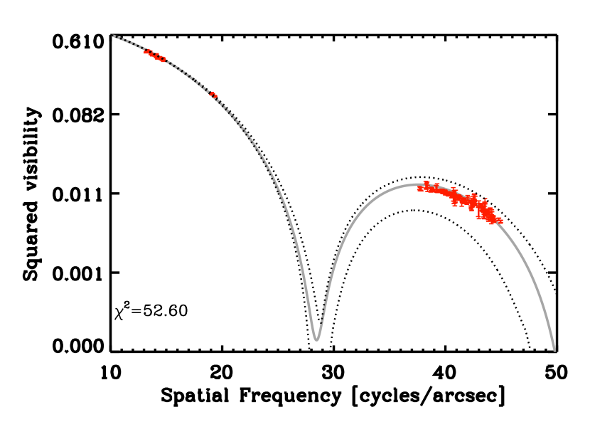
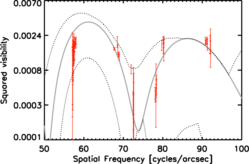
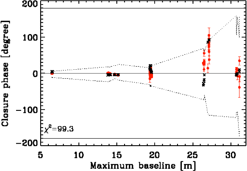
Figure 2: Top and central panels: the best-matching synthetic squared visibility (grey) compared to the observations of Betelgeuse (Haubois et al., 2009, red). The reduced $\chi^{2}$ is indicated. The dotted lines are the maximum and minimum amplitude of the visibility fluctuations as the snapshot is rotated. Bottom panel: closure phase (in degrees) versus the maximum projected baseline length for each baseline triplet. The observations (red dots with error bars) are fitted with the same intensity map and rotation angle used for the visibilities (black crosses). The axisymmetric case is represented by the solid black lines. The dotted lines are the maximum and minimum of the closure phase variation as the snapshot is rotated.

In Fig. 3 the simulation has been scaled to an apparent diameter of $\sim$45.1 mas in order to fit the data points in the first lobe, corresponding to a distance of 172.1 pc for the simulated star. The angular diameter is slightly larger than the limb-darkened diameter of 44.28$\pm$0.15 mas found by Haubois et al. (2009). Our distance is also in agreement with Harper et al. (2008), who reported a distance of $197\pm 45$ pc. Using Harper et al.’s distance and an effective temperature of 3650 K (Levesque et al., 2005), the radius is $R=890\pm 200R_{\odot}$, neglecting any uncertainty in $T_{\rm eff}$. On the other hand, using Harper et al. 2008 distance and the apparent diameter of 45 mas (Perrin et al., 2004), the radius is $R=950\pm 200R_{\odot}$. All these results match evolutionary tracks by Meynet & Maeder (2003) for an initial mass of between 15 and 25 $M_{\odot}$. The radius ($R\approx 832R_{\odot}$, see Section 2) and the effective temperature ($T_{\rm eff}\approx 3490$ K) of our 3D simulation are smaller because the simulations start with an initial model that has a guessed radius, a certain envelope mass, a certain potential profile, and a prescribed luminosity. However, during the run the internal structure relaxes so something not to far away from the initial guess (otherwise the numerical grid is inappropriate). The average final radius is determined once the simulation is finished. Therefore, since the radius (and the effective temperature) cannot be tuned, the model is placed at some distance in order to provide the angular diameter that best matches the observations. Finally, within the error bars our model radius agrees with all other data derived using the distance determined by Harper et al. (2008).

Our RHD simulation provides a better fit than uniform disk and limb-darkened models used by Haubois et al. in all lobes of the visibility function. The departure from circular symmetry is more evident at high spatial frequencies (e.g., the fourth lobe) where the visibility predicted from the parametric model is lower than the observed data. The small-scale convection-related surface structures are the cause of this departure and can only be explained by RHD simulations that are permeated with irregular convection-related structures of different size.

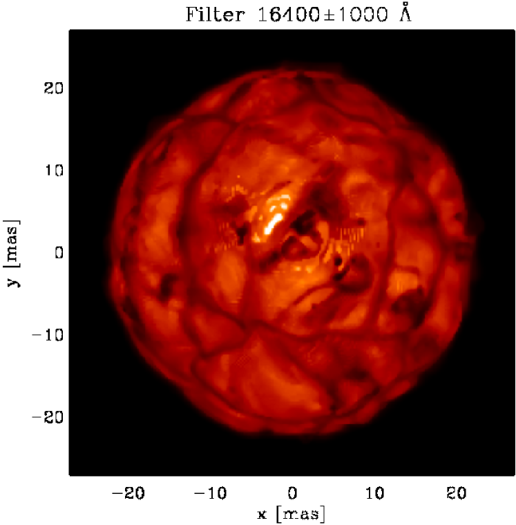
Figure 3: Map of the linear intensity in the IONIC filter. The range is [0;$3.1\times 10^{5}$] erg cm^-2 s^-1 Å^-1. The stellar parameters of this snapshot are: $L=92\,300\,L_{\odot}$, $R=832.4\,R_{\odot}$, $T_{\rm eff}=3486$ K and $\log(g)=-0.34$. The simulation has been scaled to an apparent diameter of $\sim$45.1 mas, at a distance of 172.1 pc in order to fit the data points in the first lobe.

Also the closure phases display a good agreement with the simulation indicating that a possible solution to the distribution of the inhomogeneities on the surface of Betelgeuse is the intensity map of Fig. 3 (though the reconstructed images found by Haubois et al. (2009) are more probable).

This is the first robust confirmation of the physical origin of surface granulation for Betelgeuse, following on from the detection in the K band (Paper I). Recently, Haubois et al. (2009) were able to reconstruct two images of Betelgeuse, using the data presented in this work, with two different image reconstruction algorithms. The image reconstructed with WISARD (Meimon et al., 2009, 2005) is displayed in Fig. 4 (left). Both reconstructed images in Haubois et al. paper have two spots of unequal brightness located at roughly the same positions near the center of the stellar disk. One of these spots is half the stellar radius in size. Fig. 4 shows a comparison of the reconstructed image to our best fitting snapshot of Fig. 3. Fainter structures are visible in the synthetic image (right panel) while the reconstructed image (left panel) is dominated by two bright spots. Moreover, the bigger spot visible in the reconstructed image is not present in our synthetic image, whereas there is good agreement in term of location with the smaller spot located close to the center. However, it is possible that the synthetic map does not match exactly the location of the spots because it cannot perfectly reproduce the closure phase data.

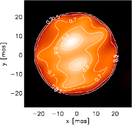
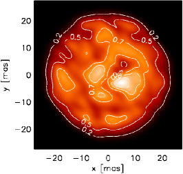
Figure 4: Left panel: recontructed image from Haubois et al. (2009). Right panel: our best fitting 3D simulation snapshot of Fig. 3 convolved with a 6$\times$6 mas PSF derived by fitting the central peak of the interferometric dirty beam. The intensities in both panels are normalized to the range [0, 1] and some contour lines are indicated (0.2, 0.5, 0.7, 0.8, 0.9 of the peak brightness).

4.1.1 Molecular contribution to the visibility curves

It is important to determine what molecular species contribute the most to the intensity absorption in the stellar atmosphere. For this purpose, we used the best fitting snapshot of Fig. 3 and recomputed the intensity maps in the IONIC filter using only CO, CN and H₂O molecules, because they are the largest absorbers at these wavelengths (Fig. 1 of this work and Fig. 3 of Paper I). The intensity maps displayed in Fig. 5 of this paper (top row) should be compared to the original one in Fig. 3 which accounts for all the molecular and atomic lines. The surfaces of CO and CN maps clearly show the granulation pattern and they are spot-free. However, the H₂O map shows dark spots which can be also identified in the original intensity map.

We also calculated visibility curves from these molecular intensity maps using the same rotation angle used to generate the synthetic data in Fig. 2. Figure 5 (bottom row) shows that the H₂O visibility is the closest to the original one both at low and high spatial frequencies. We conclude that: (i) in the first lobe, the H₂O visibility is smaller than the CO and CN visibilities. Thus the radius of the star is dependent on the H₂O contribution. (ii) At higher frequencies, only the H₂O visibility can fit the observed data whereas the CO and CN visibilities fit poorly.

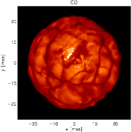
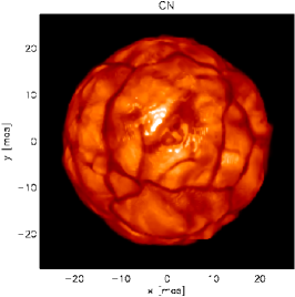
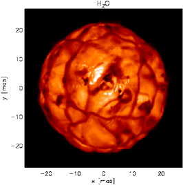
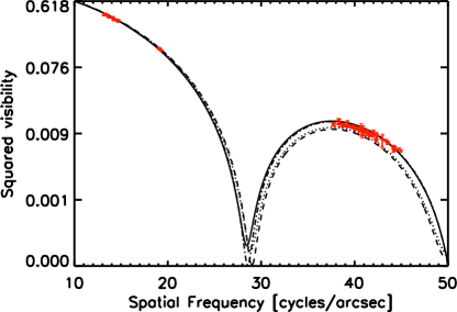
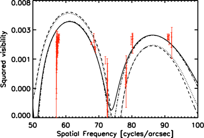
Figure 5: Top row: maps of the linear intensity in the IONIC filter of the molecular species (Fig. 1). The simulation snapshot and intensity range is the same as in Fig. 3. Bottom row: the best matching visibility curve (solid line) of Fig. 2 is compared to the visibility curve obtained from the intensity maps above: CO (dotted line), CN (dashed line), and H₂O (dash dot line). Red data points are IOTA observations.

4.1.2 Size distribution on the stellar surface

We also characterized the typical size distribution on the stellar surface using interferometric observables. The large range of spatial frequencies of the observation (between 12 to 95 arcsec^-1) is very well suited for this purpose.

Out aim is to visualize the energy within the signal as a function of spatial frequency. After the computation of the Fourier Transform, $FT$, we obtain $\hat{I}\left(u,v\right)=FT\left[I\left(x,y\right)\right]$ where $I\left(u,v\right)$ is the best matching intensity map of Fig. 3. The resulting complex number $\hat{I}\left(u,v\right)$ is multiplied by low-pass and high-pass filters to extract the information from different spatial frequency ranges (corresponding to the visibility lobes). Finally an inverse Fourier Transform, $\bar{FT}$, is used to obtain the filtered image: $I_{\rm{filtered}}\left(x,y\right)=\bar{FT}\left[\hat{I}\left(u,v\right)\cdot\rm{filter}\right]$.

Fig. 6 (top left panel) shows the filtered image at spatial frequencies, $\nu$, corresponding to the first lobe. Due to the fact that we cut off the signal at high spatial frequencies, the image appears blurry and seems to contain only the information about the stellar radius. However, the top right panel displays the signal related to all the frequencies larger than the first lobe: in this image we clearly miss the central convective cell of $\approx$ 30 mas size ($60\%$ of the stellar radius) visible in Fig. 3. Thus, the first lobe also carries information on the presence of large convective cells.

Fig. 6 (bottom row) shows the second lobe with convection-related structures of $\approx$ 10-15 mas, ($30\%$ of the stellar radius), and the third and fourth lobes with structures smaller than 10 mas. We conclude that we can estimate the presence of convection-related structures of different size using visibility measurements at the appropriate spatial frequencies. However, only imaging can definitively characterize the size of granules. A first step in this direction has been carried out in Berger et al. 2010 (to be sumbitted soon), where the image reconstruction algorythms have been tested using intensity maps from this RHD simulation. In the case of Betelgeuse, we have fitted its interferometric observables between 12 and 95 arcsec^-1 and thus inferred the presence of small to medium scale granules (5 to 15 mas) and a large convective cell ($\approx$ 30 mas).

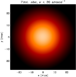
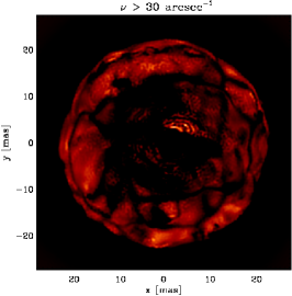
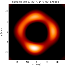
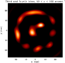
Figure 6: Intensity maps filtered at different spatial frequencies corresponding to the lobes of the visibility curve shown in Fig. 2. The images are normalized between [0,1].

4.2 Data from 7000 to 12900 Å

The simulated surface in the optical to near-infrared region shows a spectacular pattern characterized by dark spots and bright areas. The brightest areas can be up to 50 times more intense than the dark ones. In addition, this pattern changes strongly with time and has a lifetime of a few weeks. In the wavelength region below $\approx 1$ $\mu$m, the resulting surface pattern, though related to the granulation below, is also connected to dynamical effects. In fact, the light comes from higher up in the atmosphere where the optical depth is smaller than one and where waves and shocks start to dominate. In addition to this, the emerging intensity depends on the opacity run through the atmosphere and veiling by TiO molecules is very strong at these wavelengths (Fig. 1).

The filters centered in the optical part of this wavelength range are characterized by the presence of strong molecular lines while the infrared filter probes layers closer to the continuum-forming region. Observations at wavelengths in a molecular band and in the continuum probe different atmospheric depths, and thus layers at different temperatures. They provide important information on the wavelength-dependence of the limb-darkening and strong tests of our simulations.

Since the observations have been made at two different epochs, we fitted them individually: (i) the data taken in 1997 (Young et al., 2000), and (ii) the data from 2004 (Young et al., 2004). We proceeded as in Section 4.1. Note that the filter curve for the 7820 Å bandpass was lost and so a top-hat was assumed instead; we tested the validity of this assumption by replacing the known optical-region filter curves with top-hats, which did not affect the synthetic visibility and closure phase data significantly. Within the large number of computed visibilities and closure phases for each filter, we found that there are two snapshots of the simulated star, one for each epoch, that fit the observations. At each epoch the same rotation angle of the snapshot was found to fit all of the observed wavebands.

Fig. 7 displays the comparison to the data taken in 1997. The 7000 Å synthetic image corresponds to a region with strong TiO absorption (transition ${\rm A}^{3}\Phi-{\rm X}^{3}\Delta(\gamma)$, see Fig. 1). This is also true for the 9050 Å image (transition ${\rm E}^{3}\Pi-{\rm X}^{3}\Delta(\epsilon)$) but in this case the TiO band is less strong. The relative intensity of TiO bands depend on the temperature gradient of the model and change smoothly from one snapshot to another. The map at 12900 Å is TiO free and there are mostly CN lines: in this case, the surface intensity contrast is less strong than in the TiO bands.

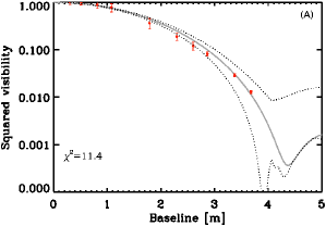
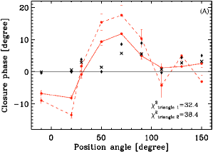
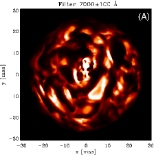
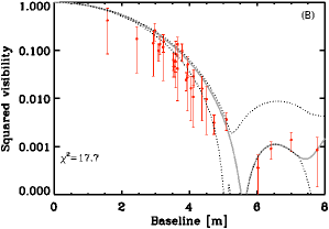
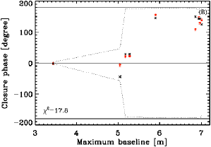
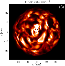
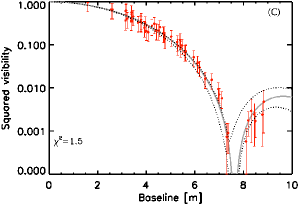
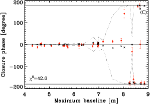
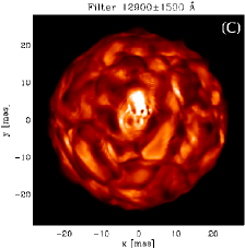
Figure 7: Comparison to the data taken in 1997 (Young et al., 2000). The symbols in the visibility curves and closure phases plots have the same meaning as in Fig. 2. The intensity are normalized between [0; $3.5\times 10^{5}$] erg cm^-2 s^-1 Å^-1. The stellar parameters of this snapshot are: $L=93\,500\,L_{\odot}$, $R=843.3\,R_{\odot}$, $T_{\rm eff}=3475$ K and $\log(g)=-0.35$. The row marked with (A), (B) and (C) correspond to bandpass centered at 7000, 9050 and 12900 Å, respectively. The visibility curves are plotted in left column, while the closure phases are shown in central column. The intensity maps centered at $7000$ and $9050$ Å have been scaled to an apparent diameter of $\sim$48.9 mas, at a distance of 161.1 pc fitting the data points in the first lobe; the map at $12900$ Å to an apparent diameter of $\sim$47.1 mas, at a distance of 167.1 pc. Row marked with (A): the observed visibility amplitudes (90 visibilities) have been averaged over the position angle of the aperture mask for the sake of clarity. We performed the fitting procedure for each of the unaveraged visibilities, and then we plot the averaged value. The closure phases of two (triangle 1 in solid and triangle 2 in dashed red line) of the 10 observed triangles have been plotted as a function of the position angle of the aperture mask on the sky. The best-matching synthetic closure phases are black crosses for triangle 1 and black diamonds for triangle 2.

Fig. 8 shows the comparison to the data taken in 2004. There, the filters used span wavelength regions corresponding to TiO absorption bands with different strengths centered at 7500Å  7800Å  and 9050Å (transitions ${\rm A}^{3}\Phi-{\rm X}^{3}\Delta(\gamma)$ and ${\rm E}^{3}\Pi-{\rm X}^{3}\Delta(\epsilon)$, see Fig. 1). Again, the same snapshot fitted the whole dataset from the same epoch.

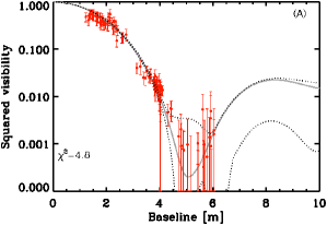
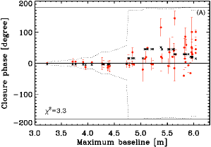
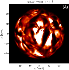
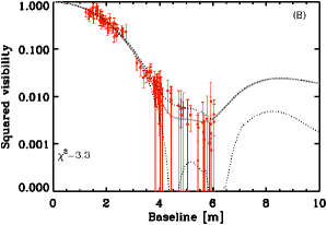
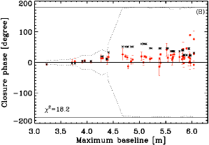
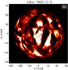
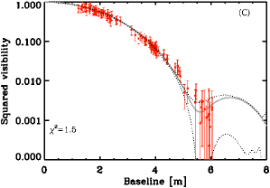
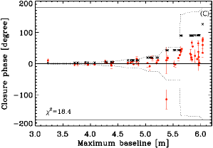
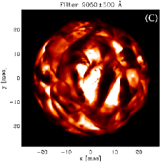
Figure 8: Same as in Fig. 7 but for the observations of Young et al. (2004). The stellar parameters of this snapshot are: $L=93\,800\,L_{\odot}$, $R=840.3\,R_{\odot}$, $T_{\rm eff}=3484$ K and $\log(g)=-0.35$. The row marked with (A), (B) and (C) correspond to bandpass centered at 7500, 7820 and 9050 Å, respectively. The intensity map centered at $7500$ Å has been scaled to an apparent diameter of $\sim$49.7 mas, at a distance of 157.9 pc; the map at $7820$ Å to an apparent diameter of $\sim$47.3 mas, at a distance of 165.7 pc; and the map $9050$ to an apparent diameter of $\sim$52.6 mas, at a distance of 149.1 pc.

The departure from circular symmetry is more evident than in the H band, with the first and the second lobes already showing large visibility fluctuations. The RHD simulation shows an excellent agreement with the data both in the visibility curves and closure phases.

However, within the same observation epoch we had to scale the size of the simulated star to a different apparent diameter at each observed wavelength. For example, in Fig. 8 the apparent diameter varies from 47.3 to 52.6 mas. Thus we infer that our RHD simulation fails to reproduce the TiO molecular band strengths probed by the three filters. As already pointed out in Paper I, our RHD simulations are constrained by execution time and they use a grey approximation for the radiative transfer that is well justified in the stellar interior and is a crude approximation in the optically thin layers; as a consequence the thermal gradient is too shallow and weakens the contrast between strong and weak lines (Chiavassa et al., 2006). The intensity maps look too sharp with respect to the observations. The implementation of non-grey opacities with five wavelength bins employed to describe the wavelength dependence of radiation fields (see Ludwig et al., 1994; Nordlund, 1982, for details) should change the mean temperature structure and the temperature fluctuations. The mean thermal gradient in the outer layers, where TiO absorption has a large effect, should increase. Moreover, in a next step, the inclusion of the radiation pressure in the simulations should lead to a different density/pressure structure with a less steep decline of density with radius. We expect that the intensity maps probing TiO bands with different strengths will eventually show larger diameter variations due to the molecular absorption as a result of these refinements.

In Young et al. (2000), the authors managed to model the data in the 7000 Å filter with two best-fitting parametric models, consisting of a circular disk with superimposed bright features (Fig. 9, central panel) or dark features (left panel). We compared these parametric models to our best-fitting synthetic image of Fig. 7 (top row). The convolved image, displayed in Fig. 9 (right panel), shows a better qualitative agreement with the bright features parametric model. In fact, 3D simulations show that the surface contrast is enhanced by the presence of significant molecular absorbers like TiO which contribute in layers where waves and shocks start to dominate. The location of bright spots is then a consequence of the underlying activity.

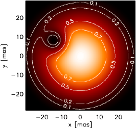
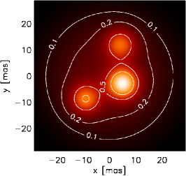
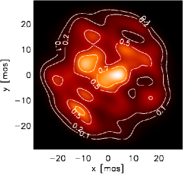
Figure 9: Left and central panels: Brightness distributions of the best fitting parametric models from Young et al. (2000) with dark features (left) and bright features (center). Right panel: our best fitting 3D simulation snapshot of Fig. 7 (row marked with (A)) convolved with a 10$\times$10 mas PSF (i.e. the size of the bright features in the parametric model). The intensities in both panels are normalized to the range [0, 1] and some contour lines are indicated (0.1,0.2,0.5,0.7).

5 Conclusions

We have used radiation hydrodynamics simulations of red supergiant stars to explain interferometric observations of Betelgeuse from the optical to the infrared region.

The picture of the surface of Betelgeuse resulting from this work is the following: (i) a granulation pattern is undoubtedly present on the surface and the convection-related structures have a strong signature in the visibility curve and closure phases at high spatial frequencies in the H band and on the first and second lobes in the optical region. (ii) In the H band, Betelgeuse is characterized by a granulation pattern that is composed of convection-related structures of different sizes. There are small to medium scale granules (5–15 mas) and a large convective cell ($\approx$30 mas). This supports previous detections carried out with our RHD simulation in the K band (Paper I), using parametric models and the same dataset (Haubois et al., 2009), Kervella et al. (2009) with VLT/NACO observations and Ohnaka et al. (2009) with VLTI/AMBER observations. Moreover, we have demonstrated that H₂O molecules contribute more than CO and CN to the position of the visibility curve’s first null (and thus to the measured stellar radius) and to the small scale surface structures. (iii) In the optical, Betelgeuse’s surface appears more complex with areas up to 50 times brighter than the dark ones. This picture is the consequence of the underlaying activity characterized by interactions between shock waves and non-radial pulsations in layers where there are strong TiO molecular bands.

These observations provide a wealth of information about both the stars and our RHD models. The comparison with the observations in the TiO bands allowed us to suggest which approximations must be replaced with more realistic treatments in the simulations. New models with wavelength resolution (i.e., non-grey opacities) are in progress and they will be tested against these observations. From the observational point of view, further multi-epoch observations, both in the optical and in the infrared, are needed to assess the time variability of convection.