Langevin equation with super-heavy-tailed noise

Abstract

We extend the Langevin approach to a class of driving noises whose generating processes have independent increments with super-heavy-tailed distributions. The time-dependent generalized Fokker-Planck equation that corresponds to the first-order Langevin equation driven by such a noise is derived and solved exactly. This noise generates two probabilistic states of the system, survived and absorbed, that are equivalent to those for a classical particle in an absorbing medium. The connection between the rate of absorption and the super-heavy-tailed distribution of the increments is established analytically. A numerical scheme for the simulation of the Langevin equation with super-heavy-tailed noise is developed and used to verify our theoretical results.

1 Introduction

At the beginning of the last century, Paul Langevin, a prominent French physicist, proposed an alternative description of Brownian motion [1]. In contrast to earlier Einstein’s approach [3], which deals with the Fokker-Planck equation for the probability density of an ensemble of independent Brownian particles, Langevin used the equation of motion for a single Brownian particle, the so-called Langevin equation. In fact, applying Newton’s second law with a random force arising from the surrounding medium, he introduced a first example of stochastic differential equations. Now the Langevin approach is one of the most effective and widely used tools for studying the effects of a fluctuating environment [5].

In physics, many other stochastic equations that account for the influence of the environment are also often termed “Langevin equations”. Among them, the dimensionless first-order (overdamped) Langevin equation

$$\dot{x}(t)=f(x(t),t)+\xi(t)$$ (1)

is the simplest and at the same time most important. It describes noise effects in very different systems, but to be specific we will call $x(t)$ a particle position [$x(0)=0$], $f(x,t)$ a deterministic force field, and $\xi(t)$ a random force (noise) resulting from a fluctuating environment. The Langevin approach is particularly useful when the noise $\xi(t)$ can be approximated by the time derivative of the noise generating process $\eta(t)$, i.e., random process with stationary and independent increments $\Delta\eta(t)=\eta(t+\tau)-\eta(t)$. The reason is that in this case the solution of equation (1) is a Markov process whose future behavior is determined only by the present state, see e.g. [6, 7].

The main statistical characteristic of the particle position $x(t)$, its probability density $P(x,t)$, depends fundamentally on the probability density $p(\Delta\eta,\tau)$ of the increments $\Delta\eta(t)$ for a sufficiently small time increment $\tau$. On a phenomenological level, $p(\Delta\eta,\tau)$ must be chosen to obtain the best representation of the environmental fluctuations. If these fluctuations are the result of many independent random variables with zero mean and finite variance, then, according to the central limit theorem [9], $p(\Delta\eta,\tau)$ can be approximated by a Gaussian probability density with zero mean and a variance proportional to $\tau$. Accordingly, $\eta(t)$ becomes a Wiener process and $\xi(t)$ reduces to Gaussian white noise. As is well known, in this case the process $x(t)$ is continuous and $P(x,t)$ satisfies the ordinary Fokker-Planck equation [5]–[8] which describes a huge variety of noise phenomena. If the above mentioned random variables have no finite variance then, as the generalized central limit theorem suggests [9], $p(\Delta\eta,\tau)$ can be chosen in the form of a Lévy stable probability density. This choice of $p(\Delta\eta,\tau)$ corresponds to Lévy stable noise $\xi(t)$ and leads to the fractional Fokker-Planck equation for $P(x,t)$ [10]–[14]. The Langevin equation (1) driven by Lévy stable noise and the corresponding fractional Fokker-Planck equation describe the so-called Lévy flights, i.e., random processes exhibiting rare but large jumps [15]–[18].

Recently, it has been shown [19] that the ordinary and fractional Fokker-Planck equations hold also for the probability densities represented in the form $p(\Delta\eta,\tau)=p(\Delta\eta/a(\tau))/a(\tau)$, where $a(\tau)$ is a scale function that tends to zero as $\tau\to 0$, and $p(y)$ is a probability density satisfying the condition $\lim_{\epsilon\to 0}p(y/\epsilon)/\epsilon=\delta(y)$ with $\delta(y)$ being the Dirac delta function. Specifically, the ordinary equation holds for a class of probability densities $p(y)$ with finite variance, and the fractional one for a class of heavy-tailed $p(y)$, i.e., probability densities with power-law tails and infinite second moment. Although these classes cover the most important cases, they do not exhaust all possible probability densities: There also exists a class of super-heavy-tailed probability densities $p(y)$ which have never been used in the Langevin approach. According to the definition, these densities decay so slowly that all fractional moments $M_{\gamma}=\int_{-\infty}^{\infty}dy\,|y|^{\gamma}p(y)$ with $\gamma>0$ are infinite (at $\gamma=0$ the normalization of $p(y)$ implies $M_{0}=1$). Because of this “unphysical” property, the super-heavy-tailed distributions, as well as the heavy-tailed ones, are not directly related to “physical” random variables having finite variance. Nevertheless, they are often used to model some specific properties of physical systems. Moreover, the heavy-tailed distributions have become a common tool for studying anomalous physical phenomena, see e.g. [15]–[17] and [20]–[22]. Although the super-heavy-tailed distributions have not yet received much attention, the examples of extremely slow diffusion [23, 24] demonstrate the usefulness of these distributions for describing systems with highly anomalous behavior.

The purpose of this paper is twofold. First, we wish to extend the Langevin equation method to a class of super-heavy-tailed noises, i.e. noises arising from the super-heavy-tailed distributions. The importance of this problem is that these noises, together with the previously known, exhaust all possible noises associated with the probability density $p(y)$ and, as a consequence, enhance the capability of this method. Second, we intend to show that super-heavy-tailed noises generate two probabilistic states of a particle, survived and absorbed. The existence of these states makes it possible to model the particle dynamics, which is randomly interrupted by the transition of a particle to a qualitatively new state, within the Langevin approach. This transition can occur in a number of physical processes, including the processes of annihilation, evaporation and absorption. In this paper we demonstrate the applicability of the Langevin equation (1) driven by super-heavy-tailed noise for describing the particle dynamics, both deterministic and random, in an absorbing medium.

2 General results

We start our analysis with the generalized Fokker-Planck equation [25]

$$\frac{\partial}{\partial t}P(x,t)=-\frac{\partial}{\partial x}f(x,t)P(x,t)+\mathcal{F}^{-1}\{P_{k}(t)\ln S_{k}\}$$ (2)

which corresponds to the Langevin equation (1). Here $\mathcal{F}\{u(x)\}=u_{k}=\int_{-\infty}^{\infty}dxe^{-ikx}u(x)$ and $\mathcal{F}^{-1}\{u_{k}\}=u(x)=(1/2\pi)\int_{-\infty}^{\infty}dk\,e^{ikx}u_{k}$ denote the direct and inverse Fourier transforms, respectively, $P_{k}(t)=\int_{-\infty}^{\infty}dxe^{-ikx}P(x,t)$ is the characteristic function of the particle position $x(t)$, and $S_{k}$ is the characteristic function of the noise generating process $\eta(t)$ at $t=1$. It is assumed that the solution of equation (2) satisfies the initial, $P(x,0)=\delta(x)$, and normalization, $\int_{-\infty}^{\infty}dxP(x,t)=1$, conditions. The characteristic function $S_{k}$ depends on the Fourier transform of the transition probability density $p(\Delta\eta,\tau)$ over the variable $\Delta\eta$. In particular, if $p(\Delta\eta,\tau)=p(\Delta\eta/a(\tau))/a(\tau)$ then

$$\ln S_{k}=\lim_{\tau\to 0}\frac{1}{\tau}[p_{ka(\tau)}-1]$$ (3)

with $p_{ka(\tau)}=\int_{-\infty}^{\infty}dy\,e^{-ika(\tau)y}p(y)$. Equation (2) reproduces all known forms of the Fokker-Planck equation associated with the Langevin equation (1) and is valid for all probability densities $p(y)$ [26]. It should be noted that because the scale function $a(\tau)$ tends to zero as $\tau\to 0$, the dependence of $\ln S_{k}$ on $k$ is determined by the asymptotic behavior of $p(y)$ at $y\to\pm\infty$.

Next we consider a class of symmetric super-heavy-tailed probability densities $p(y)$ whose asymptotic behavior at $y\to\infty$ is given by

$$p(y)\sim\frac{1}{y}h(y),$$ (4)

where $h(y)$ is a slowly varying positive function. The term “slowly varying” means that the asymptotic relation $h(\mu y)\sim h(y)$, i.e. $\lim_{y\to\infty}h(\mu y)/h(y)=1$, holds for all $\mu>0$. Since the probability density $p(y)$ is normalized, the function $h(y)$ must tend to zero more rapidly than $1/\ln y$. On the other hand, since $y^{\nu}h(y)\to\infty$ as $y\to\infty$ for all $\nu>0$ [27], $h(y)$ must decay more slowly than any positive power of $1/y$, yielding $M_{\gamma}=\infty$ ($\gamma>0$). An illustrative example of the probability density $p(y)$ satisfying these conditions is given in equation (14) below.

In order to find $\ln S_{k}$ for the examined class of probability densities, we first rewrite (3) in the form $\ln S_{k}=-2\lim_{\tau\to 0}Y(1/|k|a(\tau))/\tau$ with

$$Y(\lambda) = \int_{0}^{\infty}dy[1-\cos(y/\lambda)]p(y)$$ (5)

$$= \int_{0}^{\infty}dx\sin x\int_{\lambda x}^{\infty}dyp(y)$$

Using either of these representations and the asymptotic formula (4), one can easily show that the function $Y(\lambda)$, which according to (5) tends to zero as $\lambda\to\infty$, is slowly varying, i.e. $Y(1/|k|a(\tau))\sim Y(1/a(\tau))$ if $k\neq 0$ and $\tau\to 0$. Finally, taking into account that $\ln S_{0}=0$, we obtain the general form of $\ln S_{k}$ in the case of super-heavy-tailed $p(y)$:

$$\ln S_{k}=-q(1-\delta_{k0}),$$ (6)

where $\delta_{k0}$ is the Kronecker delta which equals $1$ if $k=0$ and $0$ otherwise, and

$$q=\lim_{\tau\to 0}\frac{2}{\tau}\,Y\bigg{(}\frac{1}{a(\tau)}\bigg{)}.$$ (7)

This limit depends on both the asymptotic behavior of $Y(\lambda)$ at $\lambda\to\infty$ and the behavior of the scale function $a(\tau)$ at $\tau\to 0$. Since the former is controlled by a given function $h(y)$, the nontrivial action of super-heavy-tailed noise, which is characterized by the condition $0<q<\infty$, occurs only at an appropriate choice of $a(\tau)$. We note that while $a(\tau)\propto\tau^{1/2}$ for all $p(y)$ with finite variance and $a(\tau)\propto\tau^{1/\alpha}$ almost for all heavy-tailed $p(y)$, where $\alpha$ is an index of stability associated with the corresponding $p(y)$ [19], there is no universal dependence of $a(\tau)$ on $\tau$ for different super-heavy-tailed $p(y)$. Moreover, because of the function $Y(\lambda)$ is slowly varying, the scale function $a(\tau)$ is in general not unique even for given $p(y)$ and $q$. We stress, however, that according to (6) the influence of super-heavy-tailed noises is fully accounted by the parameter $q$. Therefore, this lack of uniqueness is of no importance and both the Langevin and Fokker-Planck equations remain well defined (see also the next section).

To avoid possible problems with the interpretation of the Fokker-Planck equation (2) at the condition (6), let us temporarily replace the Kronecker delta by a less singular function $\Delta_{k}$ ($\Delta_{k}=1$ if $|k|\leq\kappa$ and $\Delta_{k}=0$ if $|k|>\kappa$) which reduces to $\delta_{k0}$ in the limit $\kappa\to 0$. In this case, taking $\ln S_{k}=-q(1-\Delta_{k})$, we can write the solution of equation (2) in the form $P(x,t)=\mathcal{P}(x,t)+\mathcal{A}(x,t)$, where the terms $\mathcal{P}(x,t)$ and $\mathcal{A}(x,t)$ are governed by the equations

$$\displaystyle\frac{\partial}{\partial t}\mathcal{P}(x,t)=-\frac{\partial}{\partial x}f(x,t)\mathcal{P}(x,t)-q\mathcal{P}(x,t),$$ (8)

$$\displaystyle\frac{\partial}{\partial t}\mathcal{A}(x,t)=-\frac{\partial}{\partial x}f(x,t)\mathcal{A}(x,t)-q\mathcal{A}(x,t)+q\mathcal{F}^{-1}\{P_{k}(t)\Delta_{k}\}$$ (9)

with the initial conditions $\mathcal{P}(x,0)=\delta(x)$ and $\mathcal{A}(x,0)=0$ and the normalization condition $P_{0}(t)=\mathcal{P}_{0}(t)+\mathcal{A}_{0}(t)=1$. Assuming that $z(t)$ is the solution of the deterministic equation $\dot{z}(t)=f(z(t),t)$ satisfying the initial condition $z(0)=0$, the solution of equation (8) can be written as

$$\mathcal{P}(x,t)=e^{-qt}\delta[x-z(t)].$$ (10)

By integrating $\mathcal{P}(x,t)$ over all $x$ one finds that this solution is not normalized to unity: $\mathcal{P}_{0}(t)=e^{-qt}$. Using this result and the relation $\mathcal{P}_{0}(t)+\mathcal{A}_{0}(t)=1$ we obtain $\mathcal{A}_{0}(t)=1-e^{-qt}$. It should be noted that the function $\mathcal{P}(x,t)$ and the normalization condition for $\mathcal{A}(x,t)$, $\mathcal{A}_{0}(t)=1-e^{-qt}$, do not depend on $\kappa$, i.e. they hold also at $\kappa\to 0$ when $\Delta_{k}=\delta_{k0}$.

In contrast, it is clear from the equation

$$\frac{\partial}{\partial t}\mathcal{A}(x,t) = \!-\frac{\partial}{\partial x}f(x,t)\mathcal{A}(x,t)-q\mathcal{A}(x,t)+\frac{q\sin\kappa[x-z(t)]}{\pi[x-z(t)]}e^{-qt}$$ (11)

$$\!+\frac{q}{\pi}\int_{-\infty}^{\infty}dy\frac{\sin\kappa(x-y)}{x-y}\mathcal{A}(y,t)$$

($\mathcal{A}(x,0)=0$), which follows from (9), (10) and the relation

$$\mathcal{F}^{-1}\{P_{k}(t)\Delta_{k}\}=\frac{1}{2\pi}\int_{-\kappa}^{\kappa}dk\,e^{ikx}[\mathcal{P}_{k}(t)+\mathcal{A}_{k}(t)],$$ (12)

that the function $\mathcal{A}(x,t)$ depends on $\kappa$. It is not difficult to verify that equation (11) provides a correct normalization for $\mathcal{A}(x,t)$. Indeed, the integration of both sides of this equation over all $x$ and the use of the formula $\int_{-\infty}^{\infty}dx\sin(\kappa x)/x=\pi$ lead to the equation $d\mathcal{A}_{0}(t)/dt=qe^{-qt}$ whose solution satisfying the initial condition $\mathcal{A}_{0}(0)=0$ reproduces the above result: $\mathcal{A}_{0}(t)=1-e^{-qt}$. We note, however, that because of replacing $\delta_{k0}$ by $\Delta_{k}$, equation (11) with a fixed $\kappa$ describes the influence of super-heavy-tailed noises in an approximate way. Moreover, this approximation is valid if $|x-z(t)|$ is much less than the characteristic length scale $1/\kappa$ (in the opposite case the behavior of $\mathcal{A}(x,t)$ may be unphysical with $\mathcal{A}(x,t)<0$ for some $x$ and $t$).

Assuming that $|x-z(t)|\ll 1/\kappa$ and $\kappa$ is so small that $\mathcal{P}_{k}(t)+\mathcal{A}_{k}(t)\approx 1$, we can reduce equation (11) to the form

$$\frac{\partial}{\partial t}\mathcal{A}(x,t)=-\frac{\partial}{\partial x}f(x,t)\mathcal{A}(x,t)-q\mathcal{A}(x,t)+\frac{q\kappa}{\pi}.$$ (13)

As is well known (see e.g. [28]), its general solution is given by the sum of a particular solution of this equation, which is proportional to $\kappa$, and the general solution of the related homogeneous equation (when $\kappa=0$). Since $\mathcal{A}(x,0)=0$, the latter is also proved to be proportional to $\kappa$. Thus, the function $\mathcal{A}(x,t)$ at $|x-z(t)|\ll 1/\kappa$ tends to zero linearly with $\kappa$. In particular, if the external force depends only on time, i.e. $f(x,t)=f(t)$, then $z(t)=\int_{0}^{t}dt^{\prime}f(t^{\prime})$ and the general solution of equation (13) is given by $\mathcal{A}(x,t)=e^{-qt}\,\Phi(x-z(t))+\kappa/\pi$, where $\Phi(x)$ is an arbitrary function. This function can be determined from the initial condition $\mathcal{A}(x,0)=0$, $\Phi(x)=-\kappa/\pi$, yielding $\mathcal{A}(x,t)=\kappa(1-e^{-qt})/\pi$ as $\kappa\to 0$.

The above results show that under the action of super-heavy-tailed noise two probabilistic states of a particle appear. The first one is described by the probability density $\mathcal{P}(x,t)$ and is realized with probability $\mathcal{P}_{0}(t)$. Since the noise does not affect the particle trajectory $z(t)$, see (10), we refer to this state as the surviving state. The second state, which is associated with the probability density $\mathcal{A}(x,t)$ (we recall that $\mathcal{A}(x,t)\to 0$ as $\kappa\to 0$), is realized with probability $\mathcal{A}_{0}(t)$. The transition to this state implies that a particle jumps to infinity and it is excluded from future consideration. It is therefore reasonable to call this state absorbing. To avoid any confusion, we emphasize that the act of absorption is considered here as the transition of a particle into the state in which the probability to find this particle in any finite interval equals zero. Thus, super-heavy-tailed noise plays the role of an absorbing medium characterized by the rate of absorption $q$. Accordingly, the Langevin equation (1) driven by this noise describes the overdamped motion of a particle in an absorbing medium.

As equation (10) shows, before absorption, which is random in time, the motion is deterministic and occurs under a force field $f(x,t)$. The random motion of a particle in an absorbing medium can also be described within the Langevin approach. To this end, we represent $\xi(t)$ in the Langevin equation (1) as a sum of two independent noises: (i) super-heavy-tailed noise $\xi_{1}(t)$, which models an absorbing medium, and (ii) noise $\xi_{2}(t)$, which induces the random motion of a particle. Calculations similar to those described above lead to the result $\mathcal{P}(x,t)=e^{-qt}W(x,t)$, where $W(x,t)$ denotes the normalized to unity probability density associated with the random motion of a particle. In particular, if $\xi_{2}(t)$ is Gaussian white noise then $W(x,t)$ is the solution of the ordinary Fokker-Planck equation, and if $\xi_{2}(t)$ is Lévy stable noise then $W(x,t)$ is the solution of the fractional Fokker-Planck equation. In these cases, the Langevin equation describes Brownian motion and Lévy flights, respectively, in an absorbing medium.

3 Illustrative example

In order to verify numerically that super-heavy-tailed noise acts as an absorbing medium, we first specify the super-heavy-tailed probability density $p(y)$ by choosing

$$p(y)=\frac{\ln s}{2(s+|y|)\ln^{2}(s+|y|)},$$ (14)

where $s(>1)$ is the density parameter. This symmetric probability density is unimodal with the peak located at $y=0$ and has no characteristic scale. The behavior of $p(y)$ at $y\to 0^{+}$ is characterized by the conditions $p(0)=1/(2s\ln s)$ and $dp(y)/dy|_{y\to 0^{+}}=-(1+0.5\ln s)/(s\ln s)^{2}$, and at $y\to\infty$ by the asymptotic formula $p(y)\sim\ln s/(2y\ln^{2}y)$ [this implies that $h(y)\sim\ln s/(2\ln^{2}y)$]. For this probability density the slowly varying function (5), after calculating the inner integral, takes the form

$$Y(\lambda)=\frac{\ln s}{2}\int_{0}^{\infty}dx\frac{\sin x}{\ln(s+\lambda x)}.$$ (15)

To find the leading term of $Y(\lambda)$ at $\lambda\to\infty$, which determines the rate of absorption (7), we use the identity

$$\frac{1}{\ln v}=\int_{0}^{1}\frac{du}{v^{u}}+\frac{1}{v\ln v}$$ (16)

with $v=s+\lambda x$. Substitution of this identity into (15) yields

$$Y(\lambda) = \frac{\ln s}{2}\int_{0}^{1}du\int_{0}^{\infty}dx\frac{\sin x}{(s+\lambda x)^{u}}$$ (17)

$$+\frac{\ln s}{2}\int_{0}^{\infty}dx\frac{\sin x}{(s+\lambda x)\ln(s+\lambda x)}.$$

Then, taking into account that $\int_{0}^{\infty}dx\sin(x)/x^{u}=\Gamma(1-u)\sin[\pi(1-u)/2]$, where $\Gamma(x)$ is the gamma function,

$$\int_{0}^{1}du\int_{0}^{\infty}dx\frac{\sin x}{(s+\lambda x)^{u}} \sim \int_{0}^{1}du\frac{\Gamma(1-u)}{\lambda^{u}}\sin\frac{\pi(1-u)}{2}$$ (18)

$$\sim \int_{0}^{1}du\,e^{-u\ln\lambda}\sim\frac{1}{\ln\lambda}\quad\;(\lambda\to\infty)$$

and

$$\int_{0}^{\infty}dx\frac{\sin x}{(s+\lambda x)\ln(s+\lambda x)}=o\!\left(\frac{1}{\lambda}\right)\quad\;(\lambda\to\infty),$$ (19)

we arrive to the desired asymptotic formula $Y(\lambda)\sim\ln s\,(2\ln\lambda)^{-1}$ ($\lambda\to\infty$).

As it follows from the definition of the rate of absorbtion (7), in the considered case it can be represented in the form

$$q=\frac{\ln s}{r}$$ (20)

with

$$r=\lim_{\tau\to 0}\ln\!\left(\frac{1}{a(\tau)}\right)^{\!\tau}\!.$$ (21)

Depending on the behavior of the scale function $a(\tau)$ at $\tau\to 0$, the parameter $r$ can take the values from $0$ to $\infty$. If $a(\tau)$ approaches zero so fast that $r=\infty$ then super-heavy-tailed noise does not affect the particle dynamics at all, i.e. the particle absorption is absent ($q=0$). In contrast, if $a(\tau)$ tends to zero in such a way that $r=0$ then the noise action is so strong that the transition to the absorbing state happens at $t=0^{+}$, i.e. a particle is absorbed immediately ($q=\infty$). A non-trivial action of super-heavy-tailed noise occurs at $0<r<\infty$. According to (21), in this case $a(\tau)\sim b(\tau)e^{-r/\tau}$, where $b(\tau)$ is a positive function satisfying the condition $[b(\tau)]^{\tau}\to 1$ as $\tau\to 0$. An explicit form of this function is of no importance (and so we can choose $a(\tau)=e^{-r/\tau}$) because at $a(\tau)\sim b(\tau)e^{-r/\tau}$ and $\lim_{\tau\to 0}[b(\tau)]^{\tau}=1$ the rate of absorption $q$ does not depend on $b(\tau)$:

$$q=\frac{\ln s}{\lim_{\tau\to 0}\ln[e^{r/\tau}/b(\tau)]^{\tau}}=\frac{\ln s}{r-\lim_{\tau\to 0}\ln[b(\tau)]^{\tau}}=\frac{\ln s}{r}.$$ (22)

Thus, assuming for simplicity that $f(x,t)=0$, we obtain for the examined case the probability density of the particle position in the surviving (non-absorbing) state,

$$\mathcal{P}(x,t)=s^{-t/r}\delta(x),$$ (23)

and the probability of absorption, $\mathcal{A}_{0}(t)=1-s^{-t/r}$.

It is worthy to note that while the probability density (14) with super-heavy tails depends on the single parameter $s$, the corresponding super-heavy-tailed noise is characterized also by the additional parameter $r$. The parameter $r$ relates to the scale function $a(\tau)$ and at a fixed $s$ it controls the noise intensity, namely, the smaller the parameter $r$ is the larger is this intensity. The dependence of the scale function on the parameter which characterizes the noise intensity is not surprising and occurs for all probability densities $p(y)$ [26]. If the parameters $s$ and $r$ are chosen then super-heavy-tailed noise associated with the probability density (14) is completely determined and both the Langevin and Fokker-Planck equations are well defined.

4 Numerical simulations

We have verified the analytical results obtained in the previous section by numerically studying the statistics of the particle positions. Because of the Langevin equation has never before been simulated in the case of super-heavy-tailed noises, we briefly describe the procedure for finding the particle position $x(n\tau)=\sum_{j=1}^{n}\Delta\eta(j\tau)$ at $t=n\tau$. The first step is calculating the quantity $\rho_{j}=a(\tau)(s^{1/(1-z_{j})}-s)$ with $a(\tau)=e^{-r/\tau}$ and $z_{j}$ being a random number uniformly distributed in the interval $[0,1]$. Since the positive quantities $\rho_{j}$ are distributed with the probability density $\ln s\,\{a(\tau)[s+\rho/a(\tau)]\ln^{2}[s+\rho/a(\tau)]\}^{-1}$, the increments $\Delta\eta(j\tau)$, whose probability density $p(\Delta\eta/a(\tau))/a(\tau)$ is determined by (14), can be represented in the form $\Delta\eta(j\tau)=(\pm)_{j}\,\rho_{j}/2$, where $(\pm)_{j}=+1$ or $-1$ with probability $1/2$ each. Finally, calculating $\Delta\eta(j\tau)$ $n$ times, we obtain the simulated value of the particle position: $x(n\tau)=\sum_{j=1}^{n}(\pm)_{j}\,\rho_{j}/2$.

The sample paths of $x(n\tau)$ are the piecewise constant random functions of time which are defined on the intervals $[j\tau,j\tau+\tau)$ ($0\leq j\leq n$) and satisfy the condition $x(0)=0$ (see figure 1(a)). The behavior of these sample paths at $\tau\to 0$ is determined by two major factors. The first consists in the absence of finite fractional moments of $\rho_{j}$. This means that the increments $\Delta\eta(j\tau)$ have no characteristic scale and arbitrary large values of $\Delta\eta(j\tau)$ are in principle possible. The second is that the scale function $a(\tau)$ tends to zero very rapidly as $\tau$ decreases. Since $\Delta\eta(j\tau)\propto a(\tau)$, this implies that for small enough $\tau$ the difference between the increments in neighboring intervals is in general negligible. Therefore, one may expect (and this is confirmed by our simulations) that in the limit $\tau\to 0$ the competition of these factors leads to the condition $x(t)=0$ with $t<t_{\rm{tr}}$, where $t_{\rm{tr}}$ is a random time in which the absolute value of the increment becomes bigger than any preassigned positive number (see figure 1(b)). We interpret the discontinuous jump of $x(t)$ which occurs at $t=t_{\rm{tr}}$ as the transition of a particle to the absorbing state.

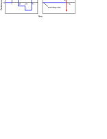
Figure 1: Illustrative examples of the sample paths of the particle position $x(t)$ for a finite time increment $\tau$ (a) and in the limit $\tau\to 0$ (b). The vertical arrow in figure 1(a) means that the jump of $x(t)$ at $t=4\tau$ exceeds the figure frame. In contrast, the arrows in figure 1(b) indicate that at $t=t_{\rm{tr}}$ an infinite jump of $x(t)$ occurs in the positive or negative direction of the axis $x$. The horizontal line with $x(t)=0$ and $t<t_{\rm{tr}}$ corresponds to the surviving state, and the vertical line to the absorbing state.

Illustrative histograms of the probability distribution of particle positions are shown in figure 2 for two different values of the time increment $\tau$.

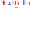
Figure 2: Histograms of the probability distribution of particle positions obtained by numerical simulations of the Langevin equation (1). The parameters of the simulation are $t=1$, $r=1$, $s=2$, $N=10^{6}$, $l=5$, $\epsilon=0.2$, and $\tau=0.25$ (a) and $\tau=10^{-3}$ (b).

The height of the $m$th bin ($m=0,\pm 1,\ldots,\pm(l-1)$) represents the probability $W_{m}$ to find a particle in this bin at time $t=n\tau$. The probability $W_{m}$ is determined as the ratio $N_{m}/N$, where $N$ is the overall number of numerical experiments, i.e. calculations of $x(t)$, and $N_{m}$ is the number of those experiments in which $x(t)$ falls into this bin, i.e. when $x(t)\in(m\epsilon-\epsilon/2,m\epsilon+\epsilon/2)$ with $\epsilon$ being the bin width. In contrast, the heights of the leftmost and rightmost bins represent the probabilities $W_{-l}$ and $W_{l}$ that $x(t)<-l\epsilon+\epsilon/2$ and $x(t)>l\epsilon-\epsilon/2$, respectively. According to these definitions $\sum_{m=-l}^{l}W_{m}=1$. The probabilities $W_{m}$ ($m\neq 0,\pm l$) rapidly tend to zero as $\tau$ decreases, and for small enough $\tau$ the histogram takes the form with only three visible bins (e.g., in figure 2(b) ${\rm{max}}\,W_{m}\sim 10^{-4}$, $W_{0}\approx 0.5$, $W_{-l}\approx W_{l}\approx 0.25$). Hence, the less is $\tau$ the better the condition $W_{0}+W_{-l}+W_{l}=1$ holds. The probability $W_{0}$ approaches the survival probability $s^{-t/r}$ (see figure 3),

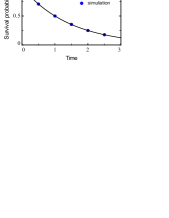
Figure 3: Time dependence of the survival probability. The solid line represents the theoretical dependence $s^{-t/r}$ (for $r=1$, $s=2$), and the circular symbols indicate the results of the numerical simulation. The latter are obtained by calculating the height of the central bin in figure 1(b) for different values of the dimensionless time $t$.

and its independence on $\epsilon$ (if $\epsilon$ is not too small for a fixed $\tau$) yields $W_{0}=\int_{-\epsilon}^{\epsilon}dx\,\mathcal{P}(x,t)$, i.e. the theoretical result (23) indeed holds. Finally, the facts that $W_{m}$ ($m\neq 0,\pm l$) approach zero as $\tau$ decreases and $W_{-l}+W_{l}\approx 1-s^{-t/r}$ (if $l$ is not too large for a fixed $\tau$) capture the main properties of $\mathcal{A}(x,t)$, namely, $\mathcal{A}(x,t)\to 0$ as $\kappa\to 0$ and $\mathcal{A}_{0}(t)=1-s^{-t/r}$. Thus, the simulation results are in full agreement with our theoretical predictions.

5 Conclusion

In summary, we have incorporated a class of super-heavy-tailed noises into the Langevin equation formalism. These noises arise from the super-heavy-tailed probability densities whose all fractional moments are infinite. Due to this feature, super-heavy-tailed noises induce two probabilistic states of a particle, survived and absorbed ones. Thus the Langevin equation driven by these noises becomes a useful tool for studying a number of physical phenomena such as absorption, evaporation, annihilation, etc. We have solved analytically the corresponding generalized Fokker-Planck equation and have confirmed our theoretical predictions via the numerical simulation of this Langevin equation.

References

References

- [1] Langevin P 1908 Sur la théorie du mouvement brownien C. R. Acad. Sci. (Paris) 146 530–33
- [2] [] For an English translation see Lemons D S and Gythiel A 1997 Paul Langevin’s 1908 paper “On the theory of Brownian motion” Am. J. Phys. 65 1079–81
- [3] Einstein A 1905 Über die von der molekularkinetischen Theorie der Wärme geforderte Bewegung von in ruhenden Flüssigkeiten suspendierten Teilchen Ann. Phys. (Leipzig) 17 549–60
- [4] [] For an English translation see Einstein A 1956 Investigations on the Theory of Brownian Movement (New York: Dover) pp 1–18
- [5] Coffey W T, Kalmykov Yu P and Waldron J T 2004 The Langevin Equation 2nd edn (Singapore: World Scientific)
- [6] Hänggi P and Thomas H 1982 Stochastic processes: Time evolution, symmetries and linear responce Phys. Rep. 88 207–319
- [7] Horsthemke W and Lefever R 1984 Noise-Induced Transitions (Berlin: Springer-Verlag)
- [8] Risken H 1989 The Fokker-Planck Equation 2nd edn (Berlin: Springer-Verlag)
- [9] Feller W 1971 An Introduction to Probability Theory and its Applications vol 2 (New York: Wiley)
- [10] Jespersen S, Metzler R and Fogedby H C 1999 Lévy flights in external force fields: Langevin and fractional Fokker-Planck equations and their solutions Phys. Rev. E 59 2736–45
- [11] Ditlevsen P D 1999 Anomalous jumping in a double-well potential Phys. Rev. E 60 172–9
- [12] Yanovsky V V, Chechkin A V, Schertzer D and Tur A V 2000 Lévy anomalous diffusion and fractional Fokker-Planck equation Physica A 282 13–34
- [13] Brockmann D and Sokolov I M 2002 Lévy flights in external force fields: From models to equations Chem. Phys. 284 409–21
- [14] Dubkov A and Spagnolo B 2005 Generalized Wiener process and Kolmogorov’s equation for diffusion induced by non-Gaussian noise source Fluct. Noise Lett. 5 L267–74
- [15] Shlesinger M F, Zaslavsky G M and Frisch U (eds) 1995 Lévy Flights and Related Topics in Physics (Berlin: Springer-Verlag)
- [16] Metzler R and Klafter J 2000 The random walk’s guide to anomalous diffusion: A fractional dynamics approach Phys. Rep. 339 1–77
- [17] Chechkin A V, Gonchar V Y, Klafter J and Metzler R 2006 Fundamentals of Lévy flight processes Adv. Chem. Phys. 133 439–96
- [18] Dubkov A, Spagnolo B and Uchaikin V V 2008 Lévy flight superdiffusion: An introduction Int. J. Bifurcat. Chaos 18 2649–72
- [19] Denisov S I, Hänggi P and Kantz H 2009 Parameters of the fractional Fokker-Planck equation Europhys. Lett. 85 40007
- [20] Bouchaud J P and Georges A 1990 Anomalous diffusion in disordered media: Statistical mechanisms, models and physical applications Phys. Rep. 195 127–293
- [21] ben-Avraham D and Havlin S 2000 Diffusion and Reactions in Fractals and Disordered Systems (Cambridge: Cambridge University Press)
- [22] Zaslavsky G M 2002 Chaos, fractional kinetics, and anomalous transport Phys. Rep. 371 461–580
- [23] Havlin S and Weiss G H 1990 A new class of long-tailed pausing time densities for the CTRW J. Stat. Phys. 58 1267–73
- [24] Dräger J and Klafter J 2000 Strong anomaly in diffusion generated by iterated maps Phys. Rev. Lett. 84 5998–6001
- [25] Denisov S I, Horsthemke W and Hänggi P 2008 Steady-state Lévy flights in a confined domain Phys. Rev. E 77 061112
- [26] Denisov S I, Horsthemke W and Hänggi P 2009 Generalized Fokker-Planck equation: Derivation and exact solutions Eur. Phys. J. B 68 567–75
- [27] Bingham N H, Goldie C M and Teugels J L 1987 Regular Variation (Cambridge: Cambridge University Press)
- [28] Polyanin A D, Zaitsev V F and Moussiaux A (2002) Handbook of First Order Partial Differential Equations (London: Taylor & Francis)