On continuous branches
of very singular similarity solutions
of the stable thin film equation

Abstract.

The fourth-order thin film equation (the TFE–4)

$$u_{t}=-\nabla\cdot(|u|^{n}\nabla\Delta u)+\Delta(|u|^{p-1}u),\,\,\mbox{where}\,\,n>0,\,\,p>1,$$

with the stable second-order diffusion term is considered. For the first critical exponent

$$p=p_{0}=\mbox{$n+1+\frac{2}{N}$}\quad\mbox{for}\,\,\,n\in(0,\mbox{$\frac{3}{2}$}),$$

where $N\geq 1$ is the space dimension, the standard free-boundary problem (FBP) with zero height, zero contact angle, and zero-flux conditions is shown to admit continuous sets (branches) of source-type very singular self-similar similarity solutions (VSSs),

$$u(x,t)=t^{-\frac{N}{4+nN}}f(y),\quad y=x/t^{\frac{1}{4+nN}}.$$

For the Cauchy problem (CP), continuous branches of oscillatory self-similar patterns of changing sign, which become “limits” of countable sets of FBP ones, are identified.

For $p\not=p_{0}$, the set of VSSs is shown to be finite and to consist of a countable family of $p$-branches of similarity profiles that originate at a sequence of critical exponents $\{p_{l},\,l\geq 0\}$. At $p=p_{l}$, these $p$-branches appear via a nonlinear bifurcation mechanism from a countable set of similarity solutions of the second kind of the pure TFE

$$u_{t}=-\nabla\cdot(|u|^{n}\nabla\Delta u)\quad\mbox{in}\quad{\mathbb{R}}^{N}\times{\mathbb{R}}_{+}.$$

Such solutions are detected by a combination of linear and nonlinear “Hermitian spectral theory” (in both the CP and FBP settings), which allows us to apply an analytical $n$-branching approach. This means constructing a continuous path as $n\to 0^{+}$ to eigenfunctions of a linear rescaled operator for $n=0$, i.e., for the bi-harmonic equation $u_{t}=-\Delta^{2}u$. Numerics are used to confirm several analytical conclusions, which do not admit a fully rigorous study.

1. Introduction: the stable TFE and main results

1.1. The model and preliminary discussion

This paper is devoted to the study of large time behaviour of solutions of higher-order quasilinear degenerate parabolic equations of not-divergent forms. More precisely, we construct global in time self-similar very singular solutions (VSSs) of the fourth-order quasilinear parabolic thin film equation (TFE–4) with the stable homogeneous second-order diffusion term,

(1.1) $$u_{t}=-\nabla\cdot(|u|^{n}\nabla\Delta u)+\Delta(|u|^{p-1}u),\quad\mbox{where}\,\,\,n>0\,\,\mbox{and}\,\,p>1.$$

The present results complete the analysis of the TFEs performed in [9, 10], where countable sets and continuous branches of blow-up and global similarity solutions were obtained for the limit unstable TFE with the backward diffusion parabolic term,

(1.2) $$u_{t}=-\nabla\cdot(|u|^{n}\nabla\Delta u)-\Delta(|u|^{p-1}u)\quad(n>0,\,\,\,p>1).$$

The main mathematical approaches for (1.2) also exhibit certain similarities with those applied in [11] to the sixth-order limit unstable TFE–6

(1.3) $$u_{t}=\nabla\cdot(|u|^{n}\nabla\Delta^{2}u)-\Delta(|u|^{p-1}u)\quad(n>0,\,\,\,p>1).$$

Surveys and extended lists of related references on the physics and mathematics of such thin film PDEs can be found in these papers [11] and [9]. As usual, for our future analysis, both pioneering papers of higher-order nonlinear diffusion theory in the 1990s by Bernis–Friedman [2] (mainly, FBP theory for TFEs), Bernis [1] and Bernis–McLeod [4], where oscillatory similarity solutions of the Cauchy problem for the fourth-order porous medium-like equations (the PME–4) were constructed, are key; see the monograph [26, Ch. 4] for further details in these areas.

We consider for (1.1) the standard FBP with zero-height, zero contact angle, and conservation of mass (zero flux) conditions,

(1.4) $$u=\nabla u=-{\bf n}\cdot(|u|^{n}\nabla\Delta u-\nabla(|u|^{p-1}u))=0$$

at the singularity surface (interface) $\Gamma_{0}[u]$, which is the lateral boundary of ${\rm supp}\,u\subset{\mathbb{R}}^{N}\times{\mathbb{R}}_{+}$ with the unit outward normal ${\bf n}$. For the range of $n\in(0,\frac{3}{2})$ plus the semilinear case $n=0$ also discussed here, these three conditions are expected to give a correctly specified problem for the fourth-order parabolic equation, which is completed with bounded, smooth, integrable, compactly supported initial data

(1.5) $$u(x,0)=u_{0}(x)\quad\mbox{in}\,\,\,\Gamma_{0}[u]\cap\{t=0\}.$$

We will also treat the Cauchy problem (CP) for (1.1) with compactly supported initial data (1.5) in ${\mathbb{R}}^{N}$. The CP admitting oscillatory solutions of “maximal” regularity will need a special setting.

We begin our study in the critical “conservative” case

(1.6) $$p=p_{0}=n+1+\mbox{$\frac{2}{N}$},$$

which is easier technically and reveals specific properties of similarity patterns. Eventually, we extend our approach to $p\not=p_{0}$ (more precisely, for $p<p_{0}$). Notice that, for $n=0$, equation (1.1) is the limit stable Cahn–Hilliard equation

(1.7) $$u_{t}=-\Delta^{2}u+\Delta(|u|^{p-1}u),$$

which occurs in various applications; see references in [12].

1.2. Main results and layout of the paper

We construct very singular self-similar (or source-type for $p=p_{0}$) solutions of (1.1) in certain ranges of the parameters $n$, $p$ and $N$. For small enough $n>0$, we will often refer to analogies with the semilinear Cahn–Hilliard equation (1.7). Typically, we assume that

(1.8) $$n\in(0,\mbox{$\frac{3}{2}$})\quad\mbox{and}\quad p>n+1,$$

but sometimes we also treat $n>\frac{3}{2}$, for which the CP continues to admit sign changing solutions that are infinitely oscillatory at the interfaces.

In Section 2 we formulate the similarity setting of the problem. Our conclusions and further layout of the paper are as follows: we show that the stable TFE (1.1) admits:

(i) In the critical case $p=p_{0}$, continuous families of global similarity solutions of the CP (Section 3) and of the FBP (Section 7);

(ii) As a co-product, we first study countable set of similarity solutions of the pure TFE (these define special bifurcation values $\{p_{l}\}$ for the full model (1.1), Section 4)

(1.9) $$u_{t}=-\nabla\cdot(|u|^{n}\nabla\Delta u)\quad\mbox{in}\quad{\mathbb{R}}^{N}\times{\mathbb{R}}_{+};\quad\mbox{and}$$

(iii) For $p<p_{0}$ (for $p>p_{0}$ no such VSSs exist), the number of similarity solutions (for a given $p$ value) becomes finite, and in the CP, there exists a countable family of $p$-branches of similarity profiles that originate at certain nonlinear bifurcation points $\{p_{l}>1,\,l\geq 0\}$ (Section 5). Some of the results are extended to the FBP (Section 9).

The principal issue that occurs is the actual relation between similarity solutions of the standard FBP and the Cauchy problem (the latter are infinitely oscillatory near the interfaces for not that large $n$). More clearly and convincingly than in our previous research, we show that, in several cases, for each asymptotic pattern of the CP, there exists a countable set of FBP patterns, which eventually converge to the CP one. It turns out that this is a rather general principal even for the linear problem for $n=0$, i.e., for the bi-harmonic equation,

(1.10) $$u_{t}=-\Delta^{2}u.$$

To show this, we will need to develop a type of Hermitian spectral theory for linear rescaled operators for both the CP (Section 4.1) and for the FBP setting (Section 9.2). The latter one becomes more difficult and unusual, with a multi-dimensional space of eigenvalues, so we discuss just initial aspects of such a theory therein.

Similar principles of self-similar asymptotics apply [11] to the sixth-order stable TFE

(1.11) $$u_{t}=\nabla\cdot(|u|^{n}\nabla\Delta^{2}u)+\Delta(|u|^{p-1}u),\quad$$

for $n\in[0,\frac{5}{4})$. In this case, the first critical exponent is $p_{0}=n+1+\mbox{$\frac{4}{N}$}.$ The semilinear case $n=0$ leads to the sixth-order unstable limit Cahn–Hilliard equation

(1.12) $$u_{t}=\Delta^{3}u+\Delta(|u|^{p-1}u),$$

whose similarity solutions can be studied as in [12].

2. Global similarity solutions: general statement and preliminaries

The similarity solutions of (1.1) have the form

(2.1) $$u_{S}(x,t)=t^{-\alpha}f(y),\quad y=x/t^{\beta},\quad\mbox{with}\quad\alpha=\mbox{$\frac{1}{2p-(n+2)}>0,\,\,\beta=\frac{p-(n+1)}{2[2p-(n+2)]}>0$}.$$

The function $f$ solves a quasilinear elliptic equation, namely,

(2.2) $${\bf A}_{+}(f)\equiv-\nabla\cdot\bigl{[}|f|^{n}\nabla\Delta f-\nabla(|f|^{p-1}f)\bigr{]}+\beta y\cdot\nabla f+\alpha f=0.\,\,$$

For $n>0$, a natural functional setting for both the FBP and the CP includes the condition

(2.3) $$f(y)\quad\mbox{is non-trivial in a bounded domain in ${\mathbb{R}}^{N}$.}$$

In the CP, $f(y)$ can be extended by $f(y)\equiv 0$ outside the support. For FBPs, posed by definition in a bounded domain, such an extension is not applicable. Note that, for the CP, the elliptic equation (2.2) admits non-compactly supported solutions with the asymptotics as $y\to\infty$ governed by the leading linear first-order operator:

(2.4) $$\beta y\cdot\nabla f+\alpha f+...=0\quad\Longrightarrow\quad f(y)=C|y|^{-\frac{\alpha}{\beta}}(1+o(1)),$$

where $C=C\big{(}\frac{y}{|y|}\big{)}$ is an arbitrary smooth function on the unit sphere $S^{N-1}$. Actually, in order to satisfy the desired condition (2.3), one needs to demand that

(2.5) $$C=0\quad\mbox{in \,\, (\ref{lf1}).}$$

For the CP with $n=0$, (2.3) is replaced by (see [12])

(2.6) $$f(y)\quad\mbox{has exponential decay at infinity,}$$

meaning that $f$ belongs to a special weighted $L^{2}$ space. The condition (2.5) is also necessarily implied.

Under (2.3) (or equivalently (2.6)), integrating (2.1) over ${\mathbb{R}}^{N}$ yields the following mass time-dependence for $p\not=p_{0}$:

(2.7) $$\int u_{S}(x,t)\,{\mathrm{d}}x=t^{\frac{N(p-p_{0})}{2[2p-(n+1)]}}\,\int f(y)\,{\mathrm{d}}y\quad\Longrightarrow\quad\int f=0\quad(p\not=p_{0}).$$

For $p=p_{0}$, any mass of $f(y)$ is formally allowed; cf. [10].

For general solutions of the TFE–4 (1.1), the self-similar scaling

(2.8) $$u(x,t)=(1+t)^{-\alpha}\theta(y,\tau),\quad y=x/(1+t)^{\beta},\quad\tau=\ln(1+t),$$

yields the evolution equation with the same operator as in (2.2),

(2.9) $$\theta_{\tau}={\bf A}_{+}(\theta)\quad\mbox{for \,\, $\tau>0$}.$$

Then a typical asymptotic stabilization problem occurs as $\tau\to+\infty$, which in particular, requires to know all possible equilibria of ${\bf A}_{+}$, this being the main current problem of concern.

The critical exponent (1.6) follows from conservation of mass; q.v. the same derivation in [9, § 3]. In addition, a countable sequence of other critical exponents $\{p_{l},\,l=0,1,2,...\}$ is expected to exist. This is confirmed in the semilinear case $n=0$ (for the limit Cahn–Hilliard equation (1.7)), where [12, § 5]

(2.10) $$p_{l}=1+\mbox{$\frac{2}{N+l}$}\quad\mbox{for any}\quad l=0,1,2,...\,.$$

See further comments in [9, § 2].

3. The CP: local oscillatory ODE bundles and profiles for $p=p_{0}$

We next study the similarity ODE in the radial setting. Let $y$ denote the single spatial variable $|y|\geq 0$. The operator of the equation (2.1) is then ordinary differential,

(3.1) $${\bf A}_{+}(f)\equiv-\frac{1}{y^{N-1}}\,\bigl{[}\,y^{N-1}|f|^{n}\big{(}\frac{1}{y^{N-1}}(y^{N-1}f^{\prime})^{\prime}\big{)}^{\prime}-y^{N-1}(|f|^{p-1}f)^{\prime}\,\bigr{]}^{\prime}+\beta yf^{\prime}+\alpha f=0.$$

We first describe the corresponding oscillatory bundle of asymptotic profiles close to interface points, which are attributed to the CP. It turns out that we have to begin with the CP. Namely, we will show that similar FBP profiles are naturally associated with the CP ones and, in particular, for both $n=0$ and $n>0$ demand certain extra “Hermitian spectral theory” as an extended and more difficult version of that in the Cauchy setting in ${\mathbb{R}}^{N}$.

3.1. The Cauchy problem: local oscillatory behaviour close to interfaces

These questions have been considered before, so, following [10, § 7.1], we briefly indicate the oscillatory asymptotic bundle of similarity profiles $f(y)$ exhibiting maximal regularity at the interface $y=y_{0}$, so that, being extended by $f=0$ for $y>y_{0}$, these will give solutions of the CP. It is easy to see that, for $n\in(0,\frac{3}{2})$, the ODE (3.2) does not admit nonnegative solutions of the maximal regularity, which can be considered as a counterpart of smooth similarity solutions of the CP for $n=0$ [12, § 5], i.e., admitting a regular limit as $n\to 0^{+}$. Hence, the ODE (3.2) implies that sufficiently regular solutions $f(y)$ must be oscillatory near interfaces; cf. proofs in [4]. It is important to prescribe the precise structure of such oscillatory singularities of the ODE and determine the dimension of the asymptotic bundle.

For $n>0$, we take the thin film ODE (3.1), keeping the main terms for $y\approx y_{0}^{-}$ and integrating once, to obtain

(3.2) $$|f|^{n}\big{(}f^{\prime\prime}+\frac{(N-1)}{y}f^{\prime}\big{)}^{\prime}-(|f|^{p-1}f)^{\prime}=\beta y_{0}f+(\mbox{higher-order terms})\,.$$

For $N=1$, choosing next just two leading terms close to the interface yields (in fact, one can see that this approximation holds for any dimension $N\geq 1$)

(3.3) $$|f|^{n}f^{\prime\prime\prime}=\beta yf+...=\lambda_{0}f+...\,,$$

where $\lambda_{0}=\beta y_{0}$. Thus, we need to consider the unperturbed ODE

(3.4) $$|f|^{n}f^{\prime\prime\prime}=\lambda_{0}f\quad(\lambda_{0}=\beta y_{0}>0),$$

whose orbits will be exponentially small perturbations near interfaces of that for (3.1).

The ODE (3.4) has the following representation of the solutions [10, § 7]: as $y\to y_{0}^{-}$,

(3.5) $$f(y)=(y_{0}-y)^{\mu}\varphi(\eta)\,,\quad\eta=\ln(y_{0}-y),\quad\mbox{with}\,\,\,\mu=\frac{3}{n},$$

where the oscillatory component $\varphi$ satisfies the autonomous ODE

(3.6) $$\varphi^{\prime\prime\prime}+3(\mu-1)\varphi^{\prime\prime}+(3\mu^{2}-6\mu+2)\varphi^{\prime}+\mu(\mu-1)(\mu-2)\varphi+\lambda_{0}|\varphi|^{-n}\varphi=0.$$

One can see that, on orbits like (3.5), the term $(|f|^{p-1}f)^{\prime}$, which has been neglected in (3.2), is much small than $f$ for all $p>1+\frac{n}{3}$ that is true since always $p>1+n$.

We are interested in periodic solutions of (3.6), which will give, according to (3.5), oscillatory profiles changing sign infinitely many times as $y\to y_{0}^{-}$, i.e., as $\eta\to-\infty$. Via (3.5), periodic functions $\varphi_{*}(\eta)$ establish the simplest oscillatory connections with the interface points keeping the maximal regularity of the envelope:

$$f(y)\sim(y_{0}-y)^{\frac{3}{n}}\quad\mbox{for}\quad y\approx y_{0}^{-},$$

which represents the true scaling-invariant nature of the ODE (3.4). According to (3.5), the regularity at $y=y_{0}$ then increases as $n\to 0^{+}$ forming, at $n=0$, analytic solutions. In [11, § 6], we present a discussion and references related to the theory of periodic solutions of higher-order ODEs. Unlike the fifth-order case in [11, § 4], the ODE (3.6) is of third order and can be reduced to a first-order ODE; see [10, § 7.1]. Therefore the existence of a periodic solution is not principally difficult, while the uniqueness (and the stability) are harder. We expect, and this is confirmed by numerics [10], that this limit cycle is “almost” globally stable (note that all the orbits of (3.6) are uniformly bounded, so a stable attractor should be available, though sometimes 0 may have a stable manifold, which was not observed) and is unique.

Increasing $n$ more, this periodic solution $\varphi_{*}(s)$ is destroyed in a heteroclinic bifurcation at the point [10, § 7.2]

(3.7) $$n_{\rm h}=1.758665...\,\big{(}\mbox{and}\,\,n_{\rm h}\in(\frac{3}{2},n_{\rm+}),\,\,\mbox{where}\,\,n_{\rm+}=\frac{9}{3+\sqrt{3}}=1.9019238...\,,\mbox{\cite[cite]{[\@@bibref{}{PetI}{}{}]}}\big{)},$$

with a standard scenario of homoclinic/heteroclinic bifurcations, [24, Ch. 4]. A rigorous justification of such non-local bifurcations is an open problem.

Thus, for $n$ larger than $\frac{3}{2}$, not all the solutions are oscillatory near the interfaces. For $n\in(\frac{3}{2},3)$, there exists a one-parametric bundle of positive solutions with constant equilibria $\varphi(\eta)\equiv\pm\varphi_{0}$ given by

(3.8) $$\pm\varphi_{0}=\pm\bigl{[}-\frac{\beta y_{0}}{\mu(\mu-1)(\mu-2)}\bigr{]}^{\frac{1}{n}}.$$

For matching purposes, this is not enough and the whole 2D asymptotic bundle (3.5) of oscillatory solutions has to be taken into account, so, for the CP, the oscillatory behaviour is expected to remain generic for all $n\in(0,n_{\rm h})$ (and similar to the linear case $n=0$ with the interface at $y_{0}=\infty$).

Thus [10], it is key that, for $n\in(0,h_{\rm h})$, there exists a 2D bundle of asymptotic oscillatory orbits near the interface with the behaviour (here $y_{0}>0$ and $s_{0}\in{\mathbb{R}}$ are parameters)

(3.9) $$f(y)=(y_{0}-y)^{\frac{3}{n}}\varphi_{*}(\ln(y_{0}-y)+s_{0})+...\quad\mbox{as}\quad y\to y_{0}^{-}.$$

Another important question is the passage to the limit $n\to 0^{+}$ that shows convergence to solutions of the semilinear Cahn–Hilliard equation. This is explained in detail in [10, § 7.6]. Various oscillatory sign change issues for nonlinear degenerate higher-order PDEs of different types are addressed in [18, Ch. 3-5].

3.2. Continuous branches of similarity profiles for $p=p_{0}$

Again, without loss of generality, we treat the case $N=1$, where the ODE is simpler and takes the form

(3.10) $$|f|^{n}f^{\prime\prime\prime}-\mbox{$\frac{1}{n+4}$}\,yf-(|f|^{n}f^{3})^{\prime}=0.$$

The origin of the existence of continuous branches (parameterized by e.g. mass) is the fact that the ODE (3.10) is of third order. Thus the single symmetry condition

(3.11) $$f^{\prime}(0)=0\quad(f(0)\not=0).$$

is posed at the origin, while the shooting bundle from the singularity point $y=y_{0}$ is 2D according to (3.9). So one parameter is free. The existence by a shooting approach is standard, so we refer to [10, 12, 19] as a guide to such equations.

The numerical results below were mainly obtained using Matlab’s two-point boundary value problem collocation solver bvp4c (with default parameter values RelTol= $10^{-3}$, AbsTol= $10^{-6}$). The standard regularization

(3.12) $$|f|^{q}\mapsto\big{(}\delta^{2}+f^{2}\big{)}^{\frac{q}{2}}$$

was used with $\delta=10^{-6}$ (and sometimes up to $10^{-10}$ in order to see complicated and refined zero structure of solutions) for $q=n$ and $\frac{2}{N}$.

In Figure 1, we present similarity profile for $n=N=1$ and $p=p_{0}=n+3=4$, which are parameterized by the values at the origin $f(0)$.

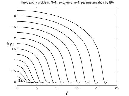
Figure 1. Similarity profiles for the CP as solutions of (3.10), (3.11) for $N=n=1$, $p=n+3=4$.

For comparison, in Figure 2(a), we present similar profiles for the semilinear case $n=0$, i.e., for the limit CH equation (1.7), where $p=p_{0}=3$. Figure 2(b) shows a clear difference of the “tail” behaviour for $n=1$ (nonlinear oscillations (3.9)) and $n=0$ (a linearized behaviour).

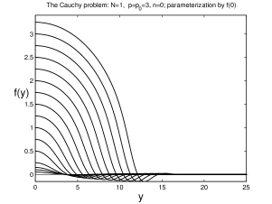
(a) $f(y)$ for $n=0$

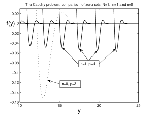
(b) zero structure enlarged

Figure 2. Similarity profiles for the CP satisfying (3.10), (3.11) for $N=1$, $n=0$ $p=3$; profiles (a) and zero structure (b).

In Figure 3, we explain how the similarity profiles at $p=p_{0}=n+3$ are deformed with $n$ starting again from the semilinear case $n=0$. It is seen that the profiles get thinner as $n$ increases and also get less oscillatory near the interface. Note that the last case with the maximal $n=1.75$ (the CP profile must still change sign, while the FBP one does not [10]) is close to the heteroclinic value (3.7), after which the similarity profiles are assumed to be finitely oscillatory, i.e., can have a finite number of sign changes near the interface (or no at all); see further comments in [10, § 9.4]. This finite oscillation phenomena lead to difficult and challenging numerical problems. Our numerics show that, for $n=1.75$, the CP profile still changes sign near the interface; see the next Figure 4.

In Figure 3, we also included the case of a single negative $n=-\frac{1}{2}$, which gives a standard source-type profile but, of course, without finite interface, where $f(y)$ is oscillatory as $y\to+\infty$. The structure of those oscillations at infinity is difficult and different from already known ones, and is not studied here.

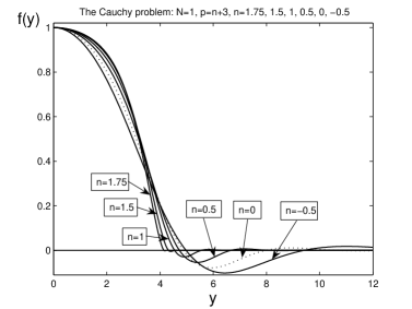
Figure 3. Similarity profiles for the CP as solutions of (3.10), (3.11) for $N=1$, $p=n+3=4$ and various $n\in[-\frac{1}{2},1\frac{3}{4}]$; parameterisation is $f(0)=1$.

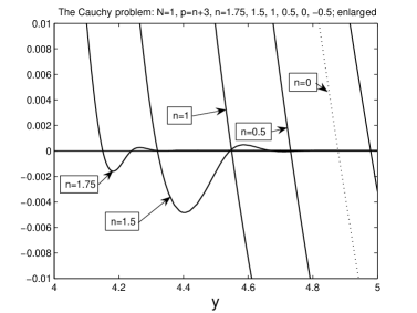
Figure 4. Enlarged zero structure of VSS profiles from Figure 3; for $p=1.75$, $f(y)$ still changes sign.

4. The Cauchy problem: countable family of source-type profiles via an $n$-branching approach

For future convenience, we now need to postpone our study of the original PDE (1.1) and digress to the pure unperturbed TFE. In general, construction of various oscillatory source-type solutions of the CP for pure TFE (1.9) is a difficult nonlinear problem, which is harder than that for the FBP.

4.1. The linear case $n=0$: basics of Hermitian spectral theory

On the other hand, for $n=0$, i.e., for the bi-harmonic equation (1.10), the first such profile exists, is unique (up to mass scaling), and is just the rescaled kernel $F(y)$ of the fundamental solution of (1.10):

(4.1) $$\begin{matrix}b(x,t)=t^{-\frac{N}{4}}F(y),\quad y=x/t^{\frac{1}{4}},\quad\mbox{where}\vskip 3.0pt plus 1.0pt minus 1.0pt\vskip 3.0pt plus 1.0pt minus 1.0pt\vskip 3.0pt plus 1.0pt minus 1.0pt\\ {\bf B}F\equiv-\Delta^{2}F+\frac{1}{4}\,y\cdot\nabla F+\frac{N}{4}\,F=0\,\,\,\mbox{in}\,\,\,{\mathbb{R}}^{N},\quad\int F=1;\end{matrix}$$

see [9, § 4]. Moreover, there exists a countable set of eigenfunctions $\{\psi_{\gamma},\,l=|\gamma|\geq 0\}$ of the corresponding rescaled non-self0-adjoint operator ${\bf B}$ with the discrete spectrum [8]

(4.2) $$\sigma({\bf B})=\big{\{}-\frac{l}{4},\,\,\,l=0,1,2,...\big{\}}.$$

The eigenfunctions are derivatives of the rescaled kernel $F$,

(4.3) $$\psi_{\gamma}(y)=\frac{(-1)^{|\gamma|}}{\sqrt{\gamma!}}\,D^{\gamma}F(y)\quad\mbox{for any multiindex}\,\,\,\gamma.$$

In addition, the adjoint operator has the same spectrum:

(4.4) $${\bf B}^{*}=-\Delta^{2}-\frac{1}{4}\,y\cdot\nabla\quad\mbox{with}\quad\sigma({\bf B}^{*})=\sigma({\bf B})=\big{\{}-\frac{l}{4},\,\,\,l=0,1,2,...\big{\}},$$

and a complete set of eigenfunctions $\{\psi_{\gamma}^{*}(y)\}$, which are generalized Hermite polynomials. See more details on such a Hermitian spectral theory of the pair $\{{\bf B},{\bf B}^{*}\}$ in [8, 15].

4.2. $n$-branching of similarity solutions

We apply the $n$-branching approach from the linear case $n=0$ in order to explain existence of a countable set of similarity solutions of the TFE (1.9). We will follow classic branching theory in the case of non-analytic nonlinearities of finite regularity; see [25, § 27] and [23, Ch. 8].

We look for solutions of (1.9) with small $n>0$ in the standard form

(4.5) $$u_{\gamma}(x,t)=t^{-\alpha}f(y),\quad y=x/t^{\beta},\quad\mbox{where}\quad\beta=\frac{1-\alpha n}{4},$$

where the multiindex $\gamma$ is used for numbering to be explained later on (in fact, similar to the linear eigenfunctions (4.3)). Then $f=f_{\gamma}(y)$ solves the elliptic equation

(4.6) $${\bf A}_{n}(f)\equiv-\nabla\cdot(|f|^{n}\nabla\Delta f)+\beta y\cdot\nabla f+\alpha f=0\quad\mbox{in}\quad{\mathbb{R}}^{N}.$$

Note that, in general, for $l\geq 1$, we have to assume that

(4.7) $$\int f(y)\,{\mathrm{d}}y=0,$$

so that the solutions (4.5) satisfy the mass conservation condition

(4.8) $$\int u_{\gamma}(x,t)\,{\mathrm{d}}x\equiv 0\quad(|\gamma|\geq 1).$$

For $l=0$, where $\alpha=\beta N$ and $\beta=\frac{1}{4+nN},$ the assumption (4.7) is not necessary, since the PDE (4.6) is fully divergent and admits integration over ${\mathbb{R}}^{N}$.

For small $n>0$ in (4.6), we have

(4.9) $$\beta=\frac{1}{4}-\frac{\alpha}{4}\,n,$$

and use the following expansion:

(4.10) $$|f|^{n}=1+n\ln|f|+o(n).$$

Here, (4.10) should be understood in the weak sense, which is necessary for using in the equivalent integral equation; see Proposition 4.1 below.

Substituting expansions (4.9) and (4.10) (still completely formal) into (4.6) yields

(4.11) $${\bf A}_{n}(f)\equiv{\bf B}f+\big{(}\alpha-\frac{N}{4}\big{)}f+n{\mathcal{L}}(f)+o(n)=0,$$

with the perturbation operator

(4.12) $${\mathcal{L}}(f)=-\nabla\cdot\bigl{(}\ln|f|\nabla\Delta f\big{)}-\frac{\alpha}{4}\,y\cdot\nabla f.$$

We next describe the behaviour of solutions for small $n>0$ and apply the classical Lyapunov-Schmidt method [23, Ch. 8] to equation (4.11). Recall that, in this linearized setting, we naturally arrive at the functional framework that is suitable for the linear operator ${\bf B}$, i.e., it is $L^{2}_{\rho}({\mathbb{R}}^{N})$, with the domain $H^{4}_{\rho}({\mathbb{R}}^{N})$, etc., and a similar setting for the adjoint operator ${\bf B}^{*}$; see above and further details in [8].

Therefore, for $n=0$, we have to study branching of a nonlinear eigenfunction from the linear one, where $f$ is a certain nontrivial finite linear combination of eigenfunctions from a given eigenspace with fixed $\lambda_{\gamma}=-\frac{|\gamma|}{4}\equiv-\frac{l}{4}$, i.e.,

(4.13) $$f=\phi_{l}=\sum_{|\gamma|=l}C_{\gamma}\psi_{\gamma}\quad(\not=0).$$

Those eigenfunctions are just derivatives (4.3) of the analytic radially symmetric rescaled kernel $F(|y|)$ of the fundamental solution (4.1). Therefore, the nodal (zero) set of such $f$ in (4.13) is well understood and consists of a countable set of isolated sufficiently smooth hypersurfaces which can concentrate as $y\to\infty$, where

(4.14) $$\phi_{l}(y)\to 0\quad\mbox{as \,\, $y\to\infty$ uniformly and exponentially fast.}$$

Hence, returning to the key limit (4.10), we have:

Proposition 4.1.

For a function $f$ given by $(\ref{a4})$, in the sense of distributions,

(4.15) $$\frac{1}{n}\,(|f|^{n}-1)\rightharpoonup\ln|f|\quad\mbox{as}\quad n\to 0^{+}.$$

According to (4.15), analyzing the integral equation for $f$, we can use the fact that, for any function $\phi\in{\mathcal{L}}$ (and $\phi\in C_{0}({\mathbb{R}}^{N})$),

(4.16) $$\int_{{\mathbb{R}}^{N}}(|f(y)|^{n}-1)\phi(y)\,{\mathrm{d}}y=n\big{[}\int_{{\mathbb{R}}^{N}}\ln|f(y)|\phi(y)\,{\mathrm{d}}y+o(1)\big{]}.$$

It follows from (4.11) that branching is possible under the following non-trivial kernel assumption: for $n=0$,

(4.17) $$\alpha-\frac{N}{4}=-\lambda_{l}=\frac{l}{4}\quad\Longrightarrow\quad\alpha_{l}(0)=\frac{N+l}{4},\quad l\geq 0.$$

This gives the countable sequence of critical exponents $\{\alpha_{l}(n),\beta_{l}(n)\}$ (to be determined) of the similarity patterns (4.5) of the TFE for small $n>0$.

By [9, Lemma 4.1], the kernel of the linearized operator

$$E_{0}={\rm ker\,}({\bf B}-\lambda_{l}I)={\rm Span\,}\{\psi_{\beta},\,|\beta|=l\}$$

is finite-dimensional. Hence, denoting by $E_{1}$ the complementary (orthogonal to $E_{0}$) invariant subspace, we set

(4.18) $$f=\phi_{l}+V_{1},\quad\mbox{where}\,\,\,\phi_{l}\in E_{0}\,\,\,\mbox{and}\,\,\,V_{1}=\sum_{|\gamma|>l}c_{\gamma}\psi_{\gamma}\in E_{1}.$$

According to the known spectral properties of operator ${\bf B}$, we define $P_{0}$ and $P_{1}$, $P_{0}+P_{1}=I$, to be projections onto $E_{0}$ and $E_{1}$ respectively. We also introduce a perturbation of the parameter $\alpha$ by setting

(4.19) $$\alpha_{l}(n)=\alpha_{l}(0)+\delta,\quad\mbox{with}\quad\delta=\delta(n).$$

This perturbation $\delta$ is obtained from the orthogonality condition by substituting into (4.11) and multiplying by $\psi_{\gamma}^{*}$. This gives

(4.20) $$\delta(n)=c_{l}n+o(n),$$

where $c_{l}$ is obtained from the system

(4.21) $$\langle{\mathcal{L}}(\phi_{l}),\psi_{\gamma}^{*}\rangle=c_{l},\quad|\gamma|=l.$$

Since according to (4.18), $\phi_{l}$ is given by (4.13), (4.21) is an algebraic system for unknowns $\{C_{\gamma}\}$ and $c_{l}$. It can be solved, for instance, in the radial geometry and in some other cases (including those where the dimension of the kernel is odd; even dimensions are known to need additional treatment); see more details in [16, App. A]. However, the total number of solutions of the non-variational system (4.21) remains unclear.

Finally, setting

(4.22) $$V_{1}=nY+o(n),$$

we obtain, passing to the limit $n\to 0^{+}$, the following equation for $Y$:

(4.23) $${\bf B}Y=-c_{l}\phi_{l}+{\mathcal{L}}(\phi_{l}).$$

By Fredholm’s theory, in view of the orthogonality, it admits a unique solution $Y\in E_{1}$.

In general, the above analysis shows that, up to solvability of the nonlinear algebraic systems, the TFE admits a countable set of different source-type similarity solutions (4.5) at least for small $n>0$, where the parameters $\alpha_{l}(n)$ are given by

(4.24) $$\alpha_{l}(n)=\frac{N+l}{4}+c_{l}n+o(n)\quad\mbox{as}\quad n\to 0^{+};\quad l=0,1,2,...\,.$$

At $n=0$, these solutions are originated from suitable eigenfunctions of the linear operator in (4.1). The global extensions of these $n$-branches of similarity solutions for larger $n>0$ represent a difficult open problem, to be treated numerically later on.

4.3. Nonlinear eigenfunctions of the TFE in one dimension

We consider the Cauchy problem for the 1D TFE with continuous compactly supported initial data,

(4.25) $$u_{t}=-(|u|^{n}u_{xxx})_{x}\quad\mbox{in}\quad{\mathbb{R}}\times{\mathbb{R}}_{+},\quad u(x,0)=u_{0}(x)\in C_{0}({\mathbb{R}}).$$

Then, for $N=1$, the nonlinear eigenvalue problem for the elliptic equation (4.6) is formulated as follows:

(4.26) $$\framebox{$-(|f|^{n}f^{\prime\prime\prime})^{\prime}+\frac{1-\alpha n}{4}\,yf^{\prime}+\alpha f=0\quad\mbox{in}\quad{\mathbb{R}},\quad f(y)\not\equiv 0,\quad f\in C_{0}({\mathbb{R}}).$}$$

Actually, (4.26) is also about self-similarity of second kind, where the desired set of parameters (nonlinear eigenvalues) $\{\alpha_{l}(n),\,l\geq 0\}$ is obtained not by a pure dimensional analysis, but via solvability of a nonlinear ODE in a given functional class $C_{0}({\mathbb{R}})$ of compactly supported functions satisfying the condition of maximal regularity. The term similarity of the second type was introduced by Ya.B. Zel’dovich in 1956, [27].

Note that, for $n=0$, (4.26) in $L^{2}_{\rho}({\mathbb{R}})$, where we replace the last condition by

$$f\in L^{2}_{\rho}({\mathbb{R}}),$$

is a standard linear eigenvalue problem for a non self-adjoint operator with the point spectrum (4.2) and complete-closed set of eigenfunctions $\{\psi_{\beta}\}$ given in (4.3), [8].

The first nonlinear eigenvalue-eigenfunction pair $\{F_{0},\,\alpha_{0}\}$ of (4.26) was proved to exist for $n\in(0,1]$; see [10, § 9]. In this case, the first eigenvalue is

(4.27) $$\alpha_{0}(n)=\frac{N}{4+nN}\big{|}_{N=1}=\frac{1}{4+n}.$$

It turns out that, in view of the highly oscillatory nature of those profiles near interfaces, even identifying the position of interfaces numerically, is not an easy problem. Therefore, we begin with Figure 5, where the first even nonlinear eigenfunction is presented for $n=0$, $\frac{1}{2}$, and $1$. A careful study of their zero structure in the log-scale in (b) allows us to find an approximate and rather rough interface location, according to the expansion (3.5), which yields

(4.28) $$\ln|f(y)|=\frac{3}{n}\,\ln(y_{0}-y)+\ln|\varphi(\ln(y_{0}-y)|+...\,.$$

For $n=0$, the expansion is exponential (cf. (9.9) below) and is entirely different, which is seen in (b); recall the regularization such as in (3.12) eventually entering the expansion for $|f|$ very small.

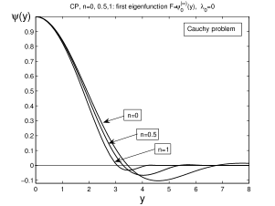
(a) eigenfunctions

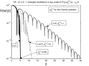
(b) zeros in log-scale

Figure 5. The first eigenfunction of (4.26), (4.27) for $n=0$, $0.5$, and $1$.

Thus, in what follows, we use the parameterisation:

(4.29) $$F_{l}(0)=1,\,\,\,l=0,2,4,...\,;\quad F_{l}^{\prime}(0)=1,\,\,\,l=1,3,...\,.$$

We then obtain that, respectively,

(4.30) $$\alpha_{1}=0.2534...\,,\quad\alpha_{2}=0.320...\,\quad(n=1).$$

In addition, numerics show that $\alpha_{3}\approx 0.38$ for $n=1$.

The results of an accurate numerical study of the first four nonlinear eigenfunctions for $N=1$ and various $n\in[0,2]$ are presented in Figure 6. Further eigenfunctions are very difficult to obtain numerically, to say nothing about an analytical proof of their existence.

In Figure 7, we show a formal schematic behaviour of the nonlinear eigenvalues $\alpha_{l}(n)$ of (4.26). The first $n$-branch, according to (4.27), has the explicit form

$$\alpha_{0}(n)=\frac{1}{4+n},\quad n\in[0,3).$$

Other $n$-branches in Figure 7 are not explicit and are hypothetical. According to the $n$-branching approach, all these branches originate at the eigenvalues of the linear problem (4.2), i.e.,

(4.31) $$\alpha_{l}(0)=-\lambda_{l+1}=\frac{l+1}{4}\quad\mbox{for}\quad l=0,1,2,...\,,$$

and moreover, after scaling, we may assume that, at $n=0$, the similarity profiles $F_{l}(y)$ coincide with the eigenfunctions (4.3), and hence by continuity mimic their geometric shapes for $n>0$.

Figure 8 shows the actual numerical construction of first four $n$-branches, and even these involve technical difficulties. Note that, at the critical heteroclinic bifurcation value (3.7), the similarity profiles $F_{l}(y)$ are supposed to loose their oscillatory behaviour at the interface and become finite oscillatory for $n>n_{\rm h}$ (or even non-oscillatory at all); see [10, § 7.2].

Analytical difficulties for the eigenvalue problem (4.26) begin already with $l=1$, i.e., with the dipole profile $F_{1}(y)$. This study has a well-developed history (see [3, 6, 7] and references therein), but still there are no definite results of existence and uniqueness of $F_{1}$ in both the FBP and Cauchy problem settings.

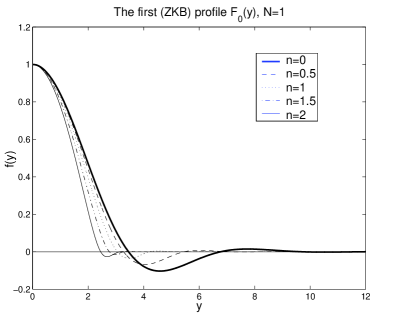
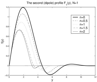
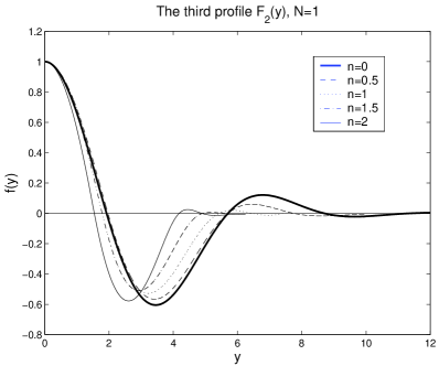
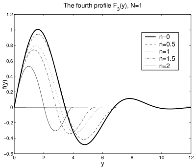
Figure 6. Illustrative numerical solutions for the first four nonlinear eigenfunctions $F_{l}(y)$, $l=0,1,2,3,$ shown for selected $n$ in one dimension $N=1$. The corresponding behaviour of the eigenvalues are shown in Figure 8. The regularisation (3.12) with $\delta=10^{-2}$ was used in the numerical shooting scheme, where the even numbered profiles satisfy $F_{l}(0)=1,F_{l}^{\prime}(0)=F_{l}^{\prime\prime\prime}(0)=0,$ whilst the odd numbered profiles have $F_{l}^{\prime}(0)=1,F_{l}(0)=F_{l}^{\prime\prime}(0)=0.$

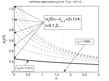
Figure 7. Formal $n$-branches of nonlinear eigenvalues $\alpha_{l}(n)$ of (4.26).

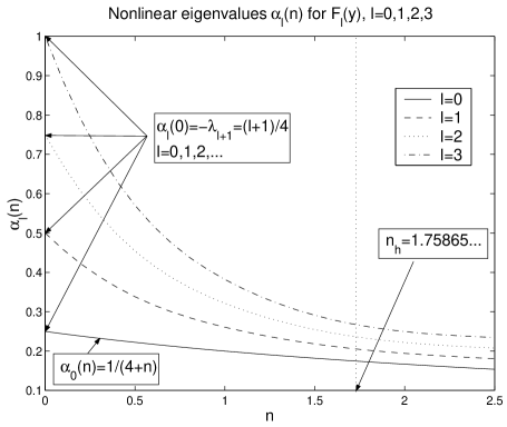
Figure 8. The actual $n$-branches of the first four nonlinear eigenvalues $\alpha_{l}(n)$, $l=0,1,2,3$, constructed numerically.

We end this discussion with the following:

Conjecture 4.1. (i) For any $n\in(0,n_{\rm h})$, the nonlinear eigenvalue problem $(\ref{nl1})$ admits a countable set of sufficiently smooth solutions of maximal regularity

(4.32) $$\Phi=\{F_{l}(y),\,\,l=0,1,2,...\},$$

where the nonlinear eigenvalues $\{\alpha_{l}\}$ form a strictly increasing sequence and

(4.33) $$\alpha_{l}\to\frac{1}{n}\quad\mbox{as}\quad l\to\infty.$$

(ii) The eigenfunction subset $(\ref{nl2})$ is evolutionary complete in $C_{0}({\mathbb{R}})$ for the TFE $(\ref{eq1})$, i.e., for any $u_{0}\not=0$, there exists a finite $l\geq 0$ and a constant $b=b(u_{0})\not=0$ such that

(4.34) $$u(x,t)=t^{-\alpha_{l}}\big{[}bF_{l}(x/t^{\beta_{l}}|b|^{n/4})+o(1)\big{]}\quad\mbox{as}\quad t\to\infty.$$

We expect that an analogous countable set of radially symmetric similarity solutions exists for the TFE (1.9) in any dimension $N\geq 2$, though numerical calculations become much more difficult than for $N=1$. Moreover, the branching approach in Section 4.2 shows that there many other non-radial similarity solutions that have a more complicated geometry but which for small $n>0$ mimic the eigenfunctions (4.3).

The evolution completeness of nonlinear eigenfunctions is known rigorously for the PME

(4.35) $$u_{t}=(|u|^{n}u)_{xx}\quad(n>0)$$

in a bounded interval [14]; see also [16] for results in ${\mathbb{R}}^{N}$ for initial data $u_{0}\in C_{0}({\mathbb{R}}^{N})$ and on an $n$-branching technique. Existence of a countable set of radial similarity solutions of (4.35) in ${\mathbb{R}}^{N}\times{\mathbb{R}}_{+}$ was proved by Hulshof [21].

5. The Cauchy problem: on nonlinear $p$-bifurcations

5.1. Semilinear Cahn–Hilliard equation: countable set of critical exponents

In order to explain the essence of the nonlinear bifurcation analysis, we first digress to the stable CH equation (1.7), for which the analysis is much simpler; cf. [12, 19].

Namely, studying the behaviour as $t\to+\infty$, we perform the standard scaling

(5.1) $$u(x,t)=(1+t)^{-\frac{1}{2(p-1)}}v(y,\tau),\quad y=x/(1+t)^{\frac{1}{4}},\quad\tau=\ln(1+t),$$

where $v(y,\tau)$ solves the following rescaled equation:

(5.2) $$v_{\tau}=-\Delta^{2}v+\frac{1}{4}\,y\cdot\nabla v+\frac{1}{2(p-1)}\,v+\Delta(|v|^{p-1}v)\equiv{\bf B}v+c_{0}v+\Delta(|v|^{p-1}v).$$

It then follows from (4.2) that a centre manifold behaviour is formally possible in the critical cases (2.10) only:

(5.3) $$c_{0}=\frac{1}{2(p-1)}-\frac{N}{4}=\frac{l}{4}\quad\Longrightarrow\quad p=p_{l}=1+\frac{2}{N+l}\quad(l\geq 0).$$

Checking the necessary condition of such a centre manifold behaviour and looking, say, for a solution moving along the centre eigenspace,

(5.4) $$v(y,\tau)=a_{\gamma}(\tau)\psi_{\gamma}(y)+w,\quad w\bot\psi_{\gamma},\quad\sup_{y}|w(y,\tau)|=o(a_{\gamma}(\tau))\,\,\,\mbox{as}\,\,\tau\to\infty,$$

and substituting into (5.2) yields on multiplication by $\psi_{\gamma}^{*}$ (see [8] for details)

(5.5) $$\dot{\alpha}_{\gamma}(\tau)=\mu_{\gamma}|a_{\gamma}|^{p-1}a_{\gamma}+...,\quad\mbox{where}\quad\mu_{\gamma}=\langle\Delta|\psi_{\gamma}|^{p-1}\psi_{\gamma},\psi_{\gamma}^{*}\rangle\equiv\langle|\psi_{\gamma}|^{p-1}\psi_{\gamma},\Delta\psi_{\gamma}^{*}\rangle.$$

Since $\psi_{\gamma}^{*}(y)$ is a $\gamma$-degree polynomial [8], we then conclude that the necessary condition of existence of such a centre subspace behaviour is as follows:

(5.6) $$\mu_{\gamma}\not=0\quad\mbox{at least, for $|\gamma|\geq 2$.}$$

Note that, in the limit $p\to 1$, the following holds:

(5.7) $$\mu_{\gamma}=1\quad\mbox{by bi-orthonormality of eigenfunctions,}$$

so that (5.6) is true for $l\gg 1$ by continuity of the integral relative to the parameter $p$.

Eventually, the centre subspace behaviour (5.5) generates the following asymptotic patterns for the CH (1.7):

(5.8) $$u_{\gamma}(x,t)\sim C_{\gamma}(t\ln^{2}t)^{-\frac{N+l}{4}}\psi_{\gamma}\big{(}\frac{y}{t^{1/4}}\big{)}+...\quad\mbox{as}\quad t\to\infty\quad(l=|\gamma|\geq 2),$$

where constants $C_{\gamma}$ are independent of initial data $u_{0}$.

5.2. Local bifurcations from $p_{l}$

We now return to the VSSs of the TFE with the stable PME term (1.1) and perform a formal nonlinear version of a $p$-bifurcation (branching) analysis for $n>0$. As usual, according to classic branching theory [23, 25], a justification (if any) is performed for the equivalent quasilinear integral equation with compact operators. For simplicity, we present computations for the differential setting.

Thus, we consider the elliptic PDE (2.2). The critical exponents $\{p_{l}\}$ are then determined from the equality (q.v. (5.3))

(5.9) $$\alpha\equiv\frac{1}{2p_{l}(n)-(n+2)}=\alpha_{l}(n)\quad\Longrightarrow\quad p_{l}(n)=\frac{n+2}{2}+\frac{1}{2\alpha_{l}(n)}\quad(l\geq 0).$$

In particular, for the semilinear case $n=0$, we have $\alpha_{l}(0)=\frac{N+l}{4}$ from (4.17), so that (5.9) leads to (5.3), i.e., to the known sequence of critical exponents (2.10).

We next use an expansion relative to the small parameter $\varepsilon=p_{0}-p$, i.e., as $\varepsilon\to 0$,

$$\begin{matrix}\alpha=\frac{1}{2p_{l}-(n+2)-2\varepsilon}=\alpha_{l}+2\alpha_{l}^{2}\varepsilon+...\,,\vskip 3.0pt plus 1.0pt minus 1.0pt\vskip 3.0pt plus 1.0pt minus 1.0pt\\ \beta=\frac{1-n\alpha_{l}}{4}+c_{l}\varepsilon+...\,,\,\,\,c_{l}=\frac{1-n\alpha_{l}}{4}\big{[}n+2+\frac{1}{\alpha_{l}}-\frac{2}{1-n\alpha_{l}}\big{]}.\end{matrix}$$

Substituting these expansions and the last one in (4.9) into (2.2) and performing the same standard linearization yields

(5.10) $${\bf A}_{n}(f)+\Delta(|f|^{p_{l}}f)+\varepsilon\big{[}-\Delta(|f|^{p_{l}}f\ln|f|)+{\mathcal{L}}_{1}F\big{]}+O(\varepsilon^{2})=0,$$

$$\mbox{where}\quad{\mathcal{L}}_{1}=c_{l}y\cdot\nabla+2\alpha_{l}^{2}I$$

is a linear operator, and ${\bf A}_{n}$ is the rescaled operator (4.6) of the pure TFE with the parameter $\alpha=\alpha_{l}(n)$ (an eigenvalue), for which there exists the corresponding similarity profile $F_{l}(y)$ (the nonlinear eigenfunction). The fact that the operator ${\bf A}_{n}$ with $\alpha=\alpha_{l}$ in (5.10) occurs in the rescaled pure TFE correctly describes the essence of a “nonlinear bifurcation phenomenon” to be revealed.

To this end, we use the additional invariant scaling of the operator ${\bf A}_{n}$ by setting

(5.11) $$f(y)=bF(y/b^{\frac{n}{4}})\quad(b>0),$$

where $b=b(\varepsilon)>0$ is a small parameter satisfying

(5.12) $$b(\varepsilon)\to 0\quad\mbox{as}\quad\varepsilon\to 0,$$

to be determined. Substituting (5.11) into (5.10) and omitting all higher-order terms (including the one with the logarithmic multiplier $\ln|b(\varepsilon)|$) yields

(5.13) $${\bf A}_{n}(F)+b^{p_{l}-\frac{n}{2}}\Delta(|F|^{p_{l}}F)+\varepsilon{\mathcal{L}}_{1}F=0.$$

Finally, we perform linearization about the nonlinear eigenfunction $F_{l}(y)$ by setting

$$F=F_{l}+Y.$$

This yields the following linear non-homogeneous problem:

(5.14) $${\bf A}_{n}^{\prime}(F_{l})Y+b^{p_{l}-\frac{n}{2}}\Delta(|F_{l}|^{p_{l}}F_{l})+\varepsilon{\mathcal{L}}_{1}F_{l}=0.$$

Here the derivative is given by

$${\bf A}_{n}^{\prime}(F)Y=-\nabla\cdot[|F|^{n}(\frac{n}{F}\,(\nabla\Delta F)Y+\nabla\Delta Y)]+\beta_{l}y\cdot\nabla Y+\alpha_{l}Y.$$

The rest of the analysis depends on assumed good spectral properties of the linearised operator ${\bf A}_{n}^{\prime}(F_{l})$. We follow the lines of a similar analysis performed for the FBP case in [17, § 2], where the operator ${\bf A}_{n}^{\prime}(F_{l})$ for $n=1$ turns out to possess a (Friedrichs’) self-adjoint extension with compact resolvent and discrete spectrum. Such a self-adjoint extension does not exist for the oscillatory $F(y)$. Here we use general theory of non-self-adjoint operators; see e.g., [20]. A proper functional setting of this operator is more straightforward for $N=1$ (and in the radial setting), where, using the behaviour of $F(y)\to 0$ as $y\to 1$, it is possible to check whether the resolvent is compact in a suitable weighted $L^{2}$ space. In general, this is a difficult problem; see below.

We assume that such a proper functional setting is available for ${\bf A}_{n}$, so we deal with operators having solutions with “minimal” singularities at the boundary of the support $S_{l}$, where the operator is degenerate and singular. Namely, we assume that ${\bf A}_{n}^{\prime}(F_{l})$ has discrete spectrum and a complete and closed set of eigenfunctions denoted again by $\{\psi_{\gamma}\}$. We also assume that the kernel is finite dimensional and we are able to determine the spectrum, eigenfunctions $\{\psi_{\gamma}^{*}\}$, and the kernel of the adjoint operator $({\bf A}_{n}^{\prime}(F_{l}))^{*}$ defined in a natural way using the topology of the dual space $L^{2}$ and having the same point spectrum (the latter is true for compact operators in a suitable space [22, Ch. 4]).

Further, we assume that there exists the orthogonal subspace ${\rm Span}\{\psi_{\gamma},|\gamma|>l\}$ of eigenfunctions of ${\bf A}_{n}^{\prime}(F_{l})$, and we look for solutions of (5.14) in the form

$$Y=\phi_{l}+w,$$

where $\phi_{l}$ belongs to the kernel and hence is analogously given by (4.13) and $w$ belongs to the orthogonal complement of the kernel. In doing so, we need to transform (5.14) into an equivalent integral equation with compact operators, but for convenience, we continue our computations using the differential version; see additional details in [19, § 3].

Thus, multiplying (5.14) by $\psi_{\gamma}^{*}$ with any $|\gamma|=l$ in $L^{2}$ and, if necessary, integrating by parts in the differential term $y\cdot\nabla F_{l}$ in ${\mathcal{L}}_{1}F_{l}$, we obtain the following orthogonality condition of solvability (Lyapunov-Schmidt’s branching equation [25, § 27]):

(5.15) $$b^{p_{l}-\frac{n}{2}}\langle\Delta(|F_{l}|^{p_{l}-1}F_{l}),\psi_{\gamma}^{*}\rangle=-\varepsilon\langle{\mathcal{L}}_{2}F_{l},\psi_{\gamma}^{*}\rangle\quad\mbox{for all}\quad|\gamma|=l.$$

These are algebraic equations for the expansion coefficients $\{C_{\gamma}\}$ in (4.13) and the function $b=b(\varepsilon)$. Similar to (5.5), one needs to check whether the constants are non zero,

(5.16) $$\langle\Delta(|F_{l}|^{p_{l}-1}F_{l}),\psi_{\gamma}^{*}\rangle\not=0\quad\mbox{and}\quad\langle{\mathcal{L}}_{2}F_{l},\psi_{\gamma}^{*}\rangle\not=0,$$

which is not a simple problem and can lead to restrictions for such a behaviour. The analysis is much simpler if the kernel is 1D, which always happens in the radial geometry where we deal with ordinary differential operators. Then (5.15) is a single and easily solved algebraic equation, for which the “transversality” problem (5.16) also occurs.

Under the conditions (5.16), the parameter $b(\varepsilon)$ in (5.11) for $p\approx p_{0}$ is given by

(5.17) $$b(\varepsilon)\sim[\gamma_{l}(p_{l}-p)]^{\frac{2\alpha_{l}}{1+2\alpha_{l}}}.$$

The direction of each $p_{l}$-branch and, whether the bifurcation is sub- or supercritical, depends on the sign on the coefficient $\gamma_{l}$ that follows from (5.15). This can be checked numerically only, but, in general, we expect that the most of these nonlinear bifurcations are subcritical so the $p_{l}$-branches exist for $p<p_{l}$.

For $n=0$, a rigorous justification of this bifurcation analysis can be found in [19, § 6], where a countable number of $p$-branches was shown to originate at bifurcation points (2.10) and were detected on the basis of known spectral properties of the corresponding linear operator in (4.1); see details in [8]. For $n>0$, as we have seen, the justification needs spectral properties of the linearised operator ${\bf A}_{n}^{\prime}(F_{l})$ and the corresponding adjoint one $({\bf A}_{n}^{\prime}(F_{l}))^{*}$, which is very difficult for non-radial nonlinear eigenfunctions $F_{l}$ and is an open problem. In particular, it would be important to know that the bi-orthonormal eigenfunction subset $\{\psi_{\gamma}\}$ of the operator ${\bf A}_{n}^{\prime}(F_{l})$ is complete and closed in a weighted $L^{2}$-space or in some specially defined closed subspace (for $n=0$, such results are available [8]). We expect that for $n\approx 0$, there exist critical exponents for the TFE with absorption that are close to those in (2.10) at $n=0$. This can be checked by standard branching-type calculus; see [16, App. A], where nonlinear eigenfunctions of the rescaled PME in ${\mathbb{R}}^{N}$ were studied by a branching approach.

6. The Cauchy problem: towards global extensions of $p$-branches

6.1. Examples of various profiles

Recall that, for $p\not=p_{0}$ in the ODE (3.1), we still have a 2D bundle at the singular interface point (3.9), but now, for even profiles, we also need to satisfy two symmetry boundary conditions at the origin:

(6.1) $$f^{\prime}(0)=f^{\prime\prime\prime}(0)=0.$$

Therefore, unlike the third-order problem (3.10), (3.11) in the critical case $p=p_{0}$, we cannot expect continuous sets of solutions. Actually, as was shown in [10, 11, 12, 19], in these non-critical cases, there occurs a countable set of $p$-branches of similarity profiles, which originate at the standard (for $n=0$) or nonlinear bifurcation points $\{p_{l}\}$ as explained in Section 5. The global behaviour of such $p$-branches can be complicated and we do not intend to study these delicate open questions in any detail, restricting ourselves to examples only.

In Figure 9, we present some VSS profile $f(y)$ for $N=1$ in two cases: $n=1$ and $p=3<p_{0}=4$ in (a) and $n=\frac{1}{2}$, $p=2$ in (b). In (b), we also show the first dipole profile $f_{1}(y)$ that, instead of (6.1), satisfies the anti-symmetry conditions at the origin,

(6.2) $$f(0)=f^{\prime\prime}(0)=0\quad\Longrightarrow\quad f(-y)\equiv-f(y).$$

Note an important feature of such compactly supported profiles that is seen in the figures: by (2.7), their mass must be zero. This necessary condition essentially “deforms” the VSS similarity profiles, so that it gets difficult to distinguish in Figure 9 their Sturmian-like properties on the numbers of dominant extrema and transversal zeros (if these apply at all). Note that the orthogonality property in (2.7) is perfectly valid for the eigenfunctions (4.3) for $n=0$ (see (4.8)), which made it possible to develop the above branching theory.

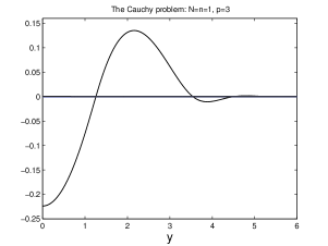
(a) $n=1$, $p=3$

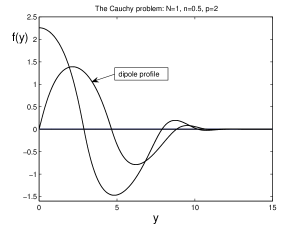
(b) $n=\frac{1}{2}$, $p=2$

Figure 9. Examples of the VSS profile for the CP satisfying (3.1), (6.1) for $N=1$; $n=1$, $p=3$ (a) and $n=\frac{1}{2}$, $p=2$ (b).

6.2. $p$-bifurcation branches: numerics

Consider the semilinear case $n=0$, which is known to be simpler, but correctly describes the expected general behaviour of the $p$-branches, at least, for sufficiently small $n>0$ (bearing in mind, that a continuous “homotopic” deformation as $n\to 0$ is observed in a number of papers mentioned above). Thus, Figure 10 illustrates this subcritical case for even symmetry conditions (6.1) at the origin. The branches are seen to remain distinct, which contrasts markedly with the supercritical case [10, 12], where the branches are increasing with $p$, so that the $p_{2}$ and higher branches “intersect” the vertical $p_{0}$ branch, $\{p=3\}$ at points (profiles) $f$ with the zero mass as in (2.7).

In Figure 10(A), we observe a strong, almost vertical, growth of these $p$-branches, which bifurcate, respectively, at

(6.3) $$p_{2}=1+\frac{2}{1+2}=\frac{5}{3},\quad p_{4}=1+\frac{2}{1+4}=\frac{7}{5},\quad p_{6}=1+\frac{2}{1+6}=\frac{9}{7}.$$

This is not surprising, since the ODE (3.1) for $N=1$ and $n=0$ assumes, as $p\to 1^{-}$, balancing the terms

(6.4) $$...\,+(|f|^{p-1}f)^{\prime\prime}+\,...\,+\frac{1}{2(p-1)}\,f=0\,\,\Longrightarrow\,\,f=C\,\hat{f},\,\,\,\mbox{where}\,\,\,C(p)\sim(p-1)^{-\frac{1}{p-1}}$$

(the scaled function $\hat{f}(y)$ is then supposed to be “almost” uniformly bounded, probably up to slower factors). Therefore, by (6.4), $f(y)$ has a super-exponential growth as $p\to 1^{+}$. Since the bifurcation values in (6.3) are already sufficiently close to 1 and the bifurcations are subcritical, these explain such a strong growth of all the $p$-bifurcation branches in Figure 10(A).

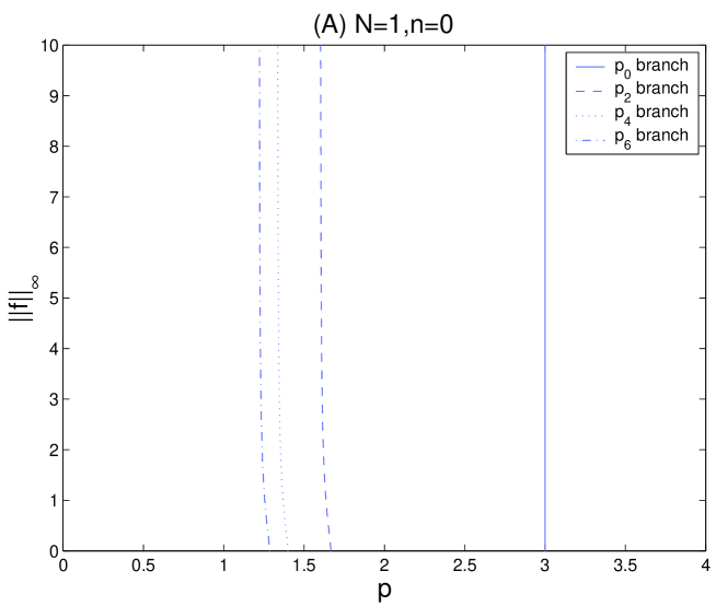
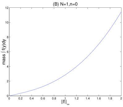
Figure 10. The bifurcation $p$-diagram and associated plots for the Cauchy case when $N=1,n=0$. (A) shows the $p$-bifurcation branches emanating from the critical exponents $p=p_{l}=1+\frac{2}{1+l}$ on the $p$-axis. The first four (even) branches $l=0,2,4,6$ are plotted. (B) illustrates the monotonicity of the mass of solutions in the critical case $p=p_{0}=3$, whilst (C) shows selected profiles on the four branches in (A) that have $||f||_{\infty}=1$.

In the nonlinear case $n>0$, such an convincing justification of the general $p$-diagram is not available. Indeed, as we have shown in the previous section, in the simplest case $l=0$, i.e., $p=p_{0}$, the bifurcation of this vertical (in $p$) branch occurs from a nonlinear eigenfunction, which is the scaled source-type profile of the nonlinear thin film operator. Other nonlinear eigenfunctions of the thin film operator are still unknown possibly excluding the second dipole-like eigenfunction. We expect that the discrete nature of the $p$-bifurcation branches discovered in [12] for $n=0$ remains valid for small $n>0$, where the nonlinear branching points cannot be calculated explicitly as in (2.10) and follows from a complicated nonlinear eigenvalue problem for the thin film operator.

7. FBP: local behaviour of radial self-similar profiles

7.1. Interface conditions in the radial setting

As in [10], for the FBP, we need to look for profiles $f(y)$, which vanish at finite $y=y_{0}>0$ and describe asymptotics of the general solution satisfying the zero contact angle and zero-flux conditions: as $y\to y_{0}^{-}$,

(7.1) $$f(y)\to 0,\,\,\,\,f^{\prime}(y)\to 0,\,\,\,\,-|f|^{n}\big{(}\frac{1}{y^{N-1}}(y^{N-1}f^{\prime})^{\prime}\big{)}^{\prime}+(|f|^{p-1}f)^{\prime}\to 0.$$

The classification below also applies to the corresponding bundles occurring for the Cahn–Hilliard equation with $n=0$, [12, § 2]. We assume that the conditions (1.8) hold (as in the blow-up case [9]).

7.2. Two-dimensional asymptotic bundle of similarity profiles

The derivation of this bundle is standard and coincides with that in [10, § 3.2]. Namely, as above, on integration, we obtain the ODE (3.2). Therefore, for $n\in[0,\frac{3}{2})$, $p>\frac{3}{2}$, the two-parametric bundle of solutions is (cf. [5, 13])

(7.2) $$f(y)=C_{0}(y_{0}-y)^{2}-A(y_{0}-y)^{q}(1+o(1)),$$

where $y_{0}>0$ and $C_{0}>0$ are arbitrary parameters and the correction term depends upon the value of $N$ and $n$, namely:

$$\mbox{(a) for $N=1$},\quad q=5-2n,\hskip 14.22636ptA=-\frac{\beta y_{0}C_{0}^{1-n}}{(5-2n)(4-2n)(3-2n)};$$

$$\mbox{(b) for $N\geq 2$},\quad\left\{\begin{array}[]{ll}q=3,\hskip 14.22636ptA=\frac{C_{0}(N-1)}{3y_{0}}&\mbox{if $n<1$},\vskip 3.0pt plus 1.0pt minus 1.0pt\\ q=3,\hskip 14.22636ptA=\frac{C_{0}(N-1)}{3y_{0}}-\frac{\beta y_{0}}{6}&\mbox{if $n=1$},\\ q=5-2n,\hskip 14.22636ptA=-\frac{\beta y_{0}C_{0}^{(1-n)}}{(5-2n)(4-2n)(3-2n)}&\mbox{if $n>1$}.\end{array}\right.$$

This expansion exists also for $n=0$ and has nothing to do with the CP exhibiting infinite propagation. It can be also used in the FBP posed for the Cahn–Hilliard equation with zero contact angle and zero-flux conditions. Proving such expansions demands a rather involved application of Banach’s contraction principle; see also [5, 13].

8. FBP: source-type similarity patterns in the critical case $p=p_{0}$

In the critical case $p=p_{0}$, the ODE (3.1) can be integrated once reducing the radial ODE to a third-order equation of the form

(8.1) $$|f|^{n}\bigl{(}f^{\prime\prime}+\frac{N-1}{y}\,f^{\prime}\bigr{)}^{\prime}-(|f|^{p_{0}-1}f)^{\prime}-\beta yf=0,\quad\mbox{where}\,\,\,\beta=\frac{1}{4+nN}.$$

At the interface, we take conditions in (7.1) written as

(8.2) $$f(y_{0})=f^{\prime}(y_{0})=0,$$

and we complete the problem statement by taking the symmetry condition at the origin (3.11). The ODE (8.1) itself then implies the second symmetry condition $f^{\prime\prime\prime}(0)=0$.

The mass $M$ of $f$ is a parameter, which is useful in distinguishing the solutions of (8.1) subject to (8.2) and (3.11). Here, we set

(8.3) $$M=\int\limits_{0}^{y_{0}}y^{N-1}f(y)\,{\mathrm{d}}y.$$

As another parameter, we can take $f^{\prime\prime}(y_{0})$ or $C_{0}=-\frac{1}{2}f^{\prime\prime}(y_{0})$, corresponding to the bundle (7.2). There are also other choices of parameters, such as $\{f(0),f^{\prime\prime}(0)\}$.

For the FBP, the local parameters $\{C_{0},y_{0}\}$ determine a two-parameter shooting problem in order to attain the single symmetry condition at the origin (3.11). The global mass-parameter $M$ is useful in classifying our solutions as bifurcations from critical mass values associated with non self-similar steady states.

Thus the statement of the FBP comprises the ODE (8.1) with the symmetry condition (3.11) within the bundle (7.2) with two parameters. Therefore, we expect a countable set of continuous families of solutions to exist, which can be parameterised relative to $y_{0}$ or with respect to the mass $M$ of the profiles. The asymptotic structure of the first (stable) branch of such similarity profiles is easier to detect.

8.1. Continuous mass-branches of solutions of the FBP

For simplicity, we again consider the 1D case. The global structure of similarity profiles does not essentially depend on $N$. In the critical case (1.6), i.e., $p_{0}=n+3$ for $N=1$, the ODE (8.1) takes the form (3.10), where at the interface point $f(y)$ is assumed to belong to the bundle (7.2). Note that this equation is obviously non-variational. The existence of a continuous set of solutions with any sufficiently small mass is proved by a shooting argument exactly as in [12, § 5]. The only difference is that all the positive large solutions as $y\to+\infty$ are concentrated in a three-dimensional bundle around the profile

$$f_{*}(y)=y^{\frac{2}{n+2}}\varphi_{*}(\ln y),$$

where the oscillatory component $\varphi_{*}(s)$ is a periodic function of changing sign of a certain autonomous ODE that is easy to derive.

8.2. Numerical construction of the global similarity patterns

The boundary-value problem is now (8.1) written as

(8.4) $$f^{\prime\prime\prime}+\frac{N-1}{y}\bigl{(}f^{\prime\prime}-\frac{1}{y}\,f^{\prime}\bigr{)}-p_{0}|f|^{\frac{2}{N}}f^{\prime}-\beta yf|f|^{-n}=0,$$

together with (8.2), (3.11), and (8.3). For fixed $N$ and $n$, the numerical results presented below suggest that there is a countable number of solutions for a given $y_{0}$. We denote the profiles with positive mass as $f_{k}$ where the index $k=1,2,\,...$ represents the number of sign changes ($k-1$) of the profile over the interval $[0,y_{0}]$ (it also being related to the number of maxima and minima). The results for the base profiles $f_{1}(y)$ are presented in Figure 11 (similarity profiles) and Figure 12 ($y_{0}$-bifurcation diagram), whilst Figure 13 gives the corresponding results for the next profiles $f_{2}(y)$ in the set. We remark that there are the corresponding reflected profiles $-f_{k}(y)$ which have negative masses.

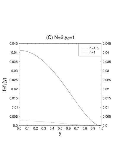
Figure 11. Illustrative numerical solutions of the base $f=f_{1}(y)$ global similarity profiles in the cases $N=1,2$. Parameter values of $y_{0}=1$ and $10$ were used for the support length together with the selected values $n=0,1,1.5$ for the index $n$. (A) and (B) show the one-dimensional case $N=1$, (C) and (D) the two-dimensional case $N=2$. In both dimensions, profiles when $y_{0}=1$ were not satisfactorily obtainable for smaller $n$ values less than $1$ (due to their values being below scheme tolerances).

Figure 12. Parameter plots of the mass $M=M_{1}$ of the base profiles solutions $f=f_{1}(y)$ with $y_{0}$ for selected $n$ values. (A) gives the one-dimensional case $N=1$ and (B) the two dimensional case $N=2$.

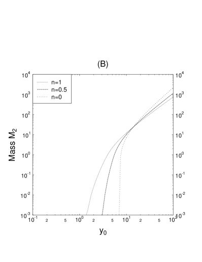
Figure 13. Parameter plots of the second profile solutions $f=f_{2}(y)$ for selected $n$ in one-dimension $N=1$. (A) gives the profiles for $y_{0}=10$, whilst (B) gives the mass as the support $y_{0}$ varies.

8.3. Asymptotic expansions

8.3.1. The small mass limit $M\to 0$

As in [10, § 4.2], we present an approach for the asymptotic expansion in the limit of small mass. This limit is easier for $n=0$ [12, Prop. 6.2], and, after rescaling, $f$ converges to the fundamental similarity rescaled profile $F$ defined in (4.1) as the first (with the eigenvalue $\lambda_{0}=0$) normalized eigenfunction of the linear non-self-adjoint operator ${\bf B}$ there. For $n>0$, we identify the corresponding zero-mass limit as follows. Let us introduce the small parameter

(8.5) $$\varepsilon=M^{\frac{2}{N}}$$

and perform the scaling

(8.6) $$f(y)=\varepsilon^{\frac{2N}{4+nN}}g(z),\quad y=\varepsilon^{\frac{nN}{2(4+nN)}}z,\quad y_{0}=\varepsilon^{\frac{nN}{2(4+nN)}}z_{0}.$$

Then the problem (8.1)–(8.3) becomes

(8.7) $$\left\{\begin{matrix}|g|^{n}\bigl{(}g^{\prime\prime}+\frac{N-1}{z}\,g^{\prime}\bigr{)}^{\prime}-\beta zg=\varepsilon(|g|^{p_{0}-1}g)^{\prime},\qquad\qquad\quad\,\,\,\vskip 3.0pt plus 1.0pt minus 1.0pt\vskip 3.0pt plus 1.0pt minus 1.0pt\\ g(z_{0})=g^{\prime}(z_{0})=0,\,\,\,g^{\prime}(0)=0,\,\,\,1=\int_{0}^{z_{0}}z^{N-1}g(z)\,{\mathrm{d}}z,\end{matrix}\right.$$

where ^′ now denotes $\frac{\mathrm{d}}{{\mathrm{d}}z}$. We pose the regular expansions

$$g=g_{0}-\varepsilon g_{1}+...,\quad z_{0}=z_{0}^{0}-\varepsilon z_{0}^{1}+...\quad\mbox{as\,\, $\varepsilon\to 0$},$$

to obtain the leading-order problem

(8.8) $$\left\{\begin{matrix}|g_{0}|^{n}\bigl{(}g_{0}^{\prime\prime}+\frac{N-1}{z}\,g_{0}^{\prime}\bigr{)}^{\prime}-\beta zg_{0}=0,\,\,\,z>0,\qquad\qquad\qquad\,\,\,\vskip 3.0pt plus 1.0pt minus 1.0pt\vskip 3.0pt plus 1.0pt minus 1.0pt\\ g_{0}(z_{0}^{0})=g_{0}^{\prime}(z_{0}^{0})=0,\,\,g_{0}^{\prime}(0)=0,\,\,1=\int_{0}^{z_{0}^{0}}z^{N-1}g_{0}(z)\,{\mathrm{d}}z.\end{matrix}\right.$$

The first-order problem, with $z_{0}^{1}=-\frac{g_{1}^{\prime}(z_{0}^{0})}{g_{0}^{\prime\prime}(z_{0}^{0})}$, is

(8.9) $$\left\{\begin{matrix}|g_{0}|^{n}\bigl{(}g_{1}^{\prime\prime}+\frac{N-1}{z}\,g_{1}^{\prime}\bigr{)}^{\prime}+(n-1)\beta zg_{1}=-p_{0}g_{0}^{\prime}|g_{0}|^{p_{0}-1},\quad\quad\vskip 3.0pt plus 1.0pt minus 1.0pt\vskip 3.0pt plus 1.0pt minus 1.0pt\\ g_{1}(z_{0}^{0})=g_{1}^{\prime}(z_{0}^{0})=0,\,\,g_{1}^{\prime}(0)=0,\,\,0=\int_{0}^{z_{0}^{0}}z^{N-1}g_{1}(z)\,{\mathrm{d}}z.\end{matrix}\right.$$

These leading and first-order problems coincide with those in the unstable case described in [10, § 4.2.1]. As such the details will not be repeated, other than to correct typographical errors in (4.18) therein, which should read

$$z_{01}^{1}=-\frac{p_{0}}{4z_{01}^{0}[8(N+2)(N+4)]^{\frac{2}{N}}}\,p_{N}(z_{01}^{0}),\,\,\,\mbox{where}\,\, p_{1}(z_{01}^{0})=-\frac{1024}{45045}\bigl{(}z_{01}^{0}\bigr{)}^{12},\,\,\,p_{2}\bigl{(}z_{01}^{0}\bigr{)}=-\frac{1}{60}(z_{01}^{0})^{8}.$$

We remark that the zero mass limit requires the support to vanish (as shown through the scaling (8.6)). The corresponding limit of vanishing support but with the mass remaining non-zero does not possess non-trivial solutions in contrast to the unstable case. This is consistent with the physical interpretation of the terms on the RHS in (1.1), since the effect of the second order term (the gravity) is no longer opposed by the fourth-order term (the surface tension) as in the unstable case (1.2).

8.4. The large mass limit $M\to\infty$

This limit occurs simultaneously with increase in support length $y_{0}$. We thus introduce the scalings

(8.10) $$y=y_{0}z,\quad f(y)=y_{0}^{\frac{2}{p_{0}-1}}g(z),\quad M=y_{0}^{N+\frac{2}{p_{0}-1}}m,$$

so that (8.1)–(8.3) becomes

(8.11) $$\left\{\begin{matrix}y_{0}^{-2(1+\frac{2}{(p_{0}-1)N})}\bigl{(}g^{\prime\prime}+\frac{N-1}{z}\,g^{\prime}\bigr{)}^{\prime}=\beta zg|g|^{-n}+p_{0}|g|^{\frac{2}{N}}g^{\prime},\vskip 3.0pt plus 1.0pt minus 1.0pt\vskip 3.0pt plus 1.0pt minus 1.0pt\\ g(1)=g^{\prime}(1)=0,\,\,\,g^{\prime}(0)=0,\,\,\,m=\int_{0}^{1}z^{N-1}g(z)\,{\mathrm{d}}z,\end{matrix}\right.$$

where ^′ again denotes $\frac{\mathrm{d}}{{\mathrm{d}}z}$. This gives a singular perturbation problem in the limit $y_{0}\to\infty$, comprising an outer region $0\leq z<1$ together with an inner region near $z=1$.

(I) Outer problem. We pose the regular expansions

$$g=g_{0}+o(1),\quad m=m_{0}+o(1)\quad\mbox{as\,\, $y_{0}\to\infty$},$$

to obtain the leading-order outer problem

(8.12) $$\left\{\begin{matrix}\beta zg_{0}|g_{0}|^{-n}+p_{0}|g_{0}|^{\frac{2}{N}}g_{0}^{\prime}=0,\,\,\,\qquad\qquad\qquad\,\,\,\qquad\vskip 3.0pt plus 1.0pt minus 1.0pt\vskip 3.0pt plus 1.0pt minus 1.0pt\\ g_{0}(1)=0=0,\,\,g_{0}^{\prime}(0)=0,\,\,m_{0}=\int_{0}^{1}z^{N-1}g_{0}(z)\,{\mathrm{d}}z.\end{matrix}\right.$$

We thus obtain the explicit solution

(8.13) $$g_{0}=\big{[}\frac{\beta(p_{0}-1)}{2p_{0}}(1-z^{2})\big{]}^{\frac{1}{p_{0}-1}},\quad m_{0}=\frac{1}{2}\big{[}\frac{\beta(p_{0}-1)}{2p_{0}}\big{]}^{\frac{1}{p_{0}-1}}\,\,\frac{\Gamma(\frac{p_{0}}{p_{0}-1})\Gamma(\frac{N}{2})}{\Gamma(\frac{p_{0}}{p_{0}-1}+\frac{N}{2})}.$$

This solution for $g_{0}$ does not satisfy the condition $g_{0}^{\prime}(1)=0$ and thus we require an inner region near $z=1$. We note that this leading order outer solution is common to all profiles $f_{k}$ in this large mass limit.

(I) Inner problem. Near $z=1$ we introduce the scalings

(8.14) $$z=1-\delta Z,\quad g=\delta^{\frac{1}{p_{0}-1}}G,$$

where dominant balance in (8.11) gives the small parameter $\delta=\delta(y_{0})=y_{0}^{-\frac{nN+4}{nN+3}}$, and for $Z=O(1)$ we pose

$$g=G_{0}+o(1)\quad\mbox{as\,\, $y_{0}\to\infty$},$$

to obtain the leading-order inner problem

(8.15) $$\left\{\begin{matrix}G_{0}^{\prime\prime\prime}=-\beta G_{0}|G_{0}|^{-n}+p_{0}|G_{0}|^{\frac{2}{N}}G_{0}^{\prime},\,\,\,\,\,\qquad\qquad\qquad\,\,\,\qquad\quad\vskip 3.0pt plus 1.0pt minus 1.0pt\\ G_{0}(0)=G_{0}^{\prime}(0)=0,\quad G_{0}\sim\big{[}\frac{(p_{0}-1)\beta Z}{p_{0}}\big{]}^{\frac{1}{p_{0}-1}}\;\;\;\mbox{as $Z\to+\infty$},\end{matrix}\right.$$

where ^′ is now $\frac{\mathrm{d}}{{\mathrm{d}}Z}$. The last condition arises from the matching with the outer solution (8.13). Consistent with the set $f_{k}$, we anticipate a countable set of solutions denoted by $G_{0k}$, $k=1,2,...\,$, and distinguished by the number of sign changes ($G_{0k}$ having $k-1$ sign changes). Numerical solutions for $G_{0}$ are shown in Figure 14, where the first two profiles are shown for the parameter value $n=1$ in the $N=1$ and $N=2$ cases.

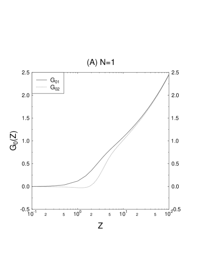
Figure 14. Numerical solution for the leading order inner problem in the large mass limit. Illustration of the first two profiles in a sequence of increasing changing sign profiles. The one-dimensional case $N=1,n=1$ is shown in (A), whilst (B) shows the two-dimensional case $N=2,n=1$. The curvature values at the origin may be used to distinguish the profiles and for comparison, we record the values $G_{01}^{\prime\prime}(0)=0.2917,G_{02}^{\prime\prime}(0)=-0.0960$ for (A), whilst we have $G_{01}^{\prime\prime}(0)=0.2130,G_{02}^{\prime\prime}(0)=-0.0667$ in (B).

9. FBP: on countable sets of $p$-branches of similarity patterns for $p\not=p_{0}$

Similar to Sections 4 and 5 for the Cauchy problem, we now intend to develop an analogous analytical approach to show existence of $p$-branches of similarity profiles in the FBP setting. This will demand rather unusual a special “spectral theory” for the corresponding linear problem for $n=0$.

9.1. The origin of countable $p$-branches

In view of essential differences and additional difficulties arising for the FBP, we restrict ourselves to the simplest case $N=1$, so that the FBP setting includes standard three free-boundary conditions

(9.1) $$f(y_{0})=f^{\prime}(y_{0})=(|f|^{n}f^{\prime\prime\prime})(y_{0})=0\quad\mbox{at an unknown boundary}\,\,\,y=y_{0}>0,$$

accomplished with two symmetry (6.1) or anti-symmetry ones (6.2) at the origin. Overall, for the 1D fourth-order ODE

(9.2) $${\bf A}_{+}(f)\equiv-(|f|^{n}f^{\prime\prime\prime})^{\prime}+\beta\,f^{\prime}y+\alpha f+(|f|^{p-1}f)^{\prime\prime}=0,\quad y\in(0,y_{0}),$$

where $\alpha=\frac{1}{2p-(n+2)}$ and $\beta=\frac{p-(n+1)}{2[2p-(n+2)]}$, these give five conditions plus an extra free parameter $y_{0}$ (a nonlinear eigenvalue). This looks like a correctly posed problem, which, in the standard analytic setting, could not have more than a countable set of solutions, or a finite number of uniformly bounded ones.

As usual, we next need to consider the corresponding 1D pure TFE (4.25), for which, in the FBP setting there appears the following nonlinear eigenvalue problem (cf. (4.26)):

(9.3) $$\left\{\begin{matrix}-(|f|^{n}f^{\prime\prime\prime})^{\prime}+\frac{1-\alpha n}{4}\,yf^{\prime}+\alpha f=0\,\,\,\mbox{on}\,\,\,(y_{-},y_{+}),\,\,\,\vskip 3.0pt plus 1.0pt minus 1.0pt\\ f=f^{\prime}=|f|^{n}f^{\prime\prime\prime}=0\,\,\mbox{at}\,\,y=y_{\pm}.\qquad\qquad\quad\,\,\,\,\end{matrix}\right.$$

Note that, unlike the CP one (4.26), the space of eigenvalues is three parametric, and, besides the usual nonlinear eigenvalue $\alpha\in{\mathbb{R}}$ includes two free boundary positions $y_{\pm}$. In the two basic simpler cases with the symmetry (6.1) or antisymmetry (6.2), the eigenvalue space is 2D:

(9.4) $$\mbox{Eigenvalues:}\quad\mu=(\alpha,y_{0})^{T}\in{\mathbb{R}}^{2},$$

to which we concentrate upon in what follows.

9.2. $n=0$: first aspects of linear “Hermitian spectral theory”

For $n=0$, the nonlinear eigenvalue problem (9.3) becomes a linear one for the operator ${\bf B}$ in (4.1):

(9.5) $${\bf B}\psi\equiv-\psi^{(4)}+\frac{1}{4}\,\psi^{\prime}y+\frac{1}{4}\,\psi=\lambda\psi\,\,\,(\lambda=\frac{1}{4}-\alpha),\quad\psi=\psi^{\prime}=\psi^{\prime\prime\prime}=0\,\,\,\mbox{at}\,\,\,y=y_{\pm}.$$

Even in the simpler case (9.4), this is not a standard spectral problem, and, moreover, it is not clear whether this can be attributed to such classes. Let us comment that each “eigenfunction” $\psi_{k}(y)$ is supposed to be defined on its own interval $(y_{k-},y_{k+})$, but using eigenfunction subsets together with notions of completeness, closure, etc. may not make sense.

We now discuss some particular aspects of the problem (9.5) and restrict our analysis to the first eigenvalue $\lambda_{0}=0$ and the corresponding even eigenfunctions. On integration, the ODE becomes of the third order,

(9.6) $$-\psi^{\prime\prime\prime}+\frac{1}{4}\,y\psi=0\,\,\,\mbox{on}\,\,\,(0,y_{0}),\,\,\,\psi(0)=1,\,\,\,\psi^{\prime}(0)=0;\quad\psi(y_{0})=\psi^{\prime}(y_{0})=0,$$

where for convenience we fix the normalization $\psi(0)=1$ and take symmetry conditions at the origin (the subscript + then being dropped on the domain end point). We can prove the following:

Proposition 9.1.

The $y_{0}$-eigenvalue problem $(\ref{.4})$, corresponding to $\lambda_{0}=0$, admits a countable set of eigenfunctions $\{\psi_{0}^{(k)},\,k\geq 1\}$ defined on the intervals $\{(0,y_{0}^{(k)})\}$, and,

(9.7) $$\mbox{ as $k\to\infty$},\quad y_{0}^{(k)}\sim k^{\frac{3}{4}}\to+\infty\quad\mbox{and}\quad\psi_{0}^{(k)}(y)\to F(y),$$

where $F(y)\equiv\psi_{0}^{(\infty)}(y)$ is the first eigenfunction $(\ref{ps1})$ of the rescaled operator ${\bf B}$ in $(\ref{tf3})$ defined for the CP $($i.e., in the whole ${\mathbb{R}})$.

Proof. A proper solvability of the problem (9.6) follows from the known WKBJ-type asymptotics of solutions of this ODE for large $y$:

(9.8) $$\psi(y)\sim{\mathrm{e}}^{ay^{4/3}}\quad\Longrightarrow\quad a^{3}=\frac{1}{4}\big{(}\frac{3}{4}\big{)}^{3}.$$

This gives three roots: the real positive one $a_{0}=3\cdot 4^{-\frac{4}{3}}$ and two complex:

$$a_{\pm}=\big{(}-\frac{1}{2}\pm{\rm i}\,\frac{\sqrt{3}}{2}\big{)}a_{0}.$$

A full WKBJ expansion includes also a slow growing algebraic multiplying factor $y^{-1/3}$ (not important for the final estimates): as $y\to\infty$,

(9.9) $$\psi(y)\sim y^{-\frac{1}{3}}\Big{\{}C_{1}{\mathrm{e}}^{a_{0}y^{4/3}}+C_{2}{\mathrm{e}}^{-\frac{a_{0}}{2}\,y^{4/3}}\cos\big{(}\frac{a_{0}\sqrt{3}}{2}y^{\frac{4}{3}}+C_{3}\big{)}\Big{\}}+...\,,$$

where $C_{1,2,3}$ are real constants. Solving the problem at the free boundary $y_{0}\gg 1$, we see that acceptable roots are concentrated about the roots of the $\cos$ or $\sin$ functions, so that $y_{0}^{(k)}$ satisfy

(9.10) $$\cos\big{(}\frac{a_{0}\sqrt{3}}{2}(y_{0}^{(k)})^{\frac{4}{3}}+C_{3}\big{)}\approx 0\quad\Longrightarrow\quad\frac{a_{0}\sqrt{3}}{2}(y_{0}^{(k)})^{\frac{4}{3}}\sim\pi\big{(}\frac{1}{2}+k\big{)}-C_{3},$$

whence the estimate in (9.7). Since $y_{0}^{(k)}\to\infty$, the convergence to the rescaled kernel $F$ in the CP is obvious (see Figures below for a further justification). ∎

In Figure 15, we show the first positive eigenfunction $\psi_{0}^{(1)}$ of (9.6). Figure 16 shows first four eigenfunctions of (9.6). This illustrates the convergence to $F$ in (9.7), where $\psi_{0}^{(4)}(y)$ is already very close to $F$, so that the next $\psi_{0}^{(5)}$ is difficult to detect numerically.

For $\lambda\neq 0$, the corresponding statement to (9.6) is

(9.11) $$\left\{\begin{matrix}-\psi^{\prime\prime\prime}+\frac{1}{4}\,y\psi=\lambda\int\limits_{0}^{y}\psi(s)\,{\mathrm{d}}s\,\,\,\mbox{on}\,\,\,(0,y_{+}),\qquad\qquad\qquad\,\,\vskip 3.0pt plus 1.0pt minus 1.0pt\\ \,\,\,\psi(0)=1,\,\,\,\psi^{\prime}(0)=0;\quad\psi(y_{+})=\psi^{\prime}(y_{+})=\psi^{\prime\prime\prime}(y_{+})=0.\end{matrix}\right.$$

We distinguish the sets of even eigenfunctions $\{\psi=\psi_{m},\lambda=\lambda_{m},y_{+}=y_{m}\}$, using the subscript $m=0,2,4,\ldots$. Within each set with $m$ fixed, we have a countable set of eigenfunctions $\{\psi_{m}=\psi_{m}^{(k)},y_{m}=y_{m}^{(k)}\},k=1,2,3,...\,$. The first three eigenfunctions for the second $m=2$ and the fourth $m=4$ sets are shown in Figure 17.

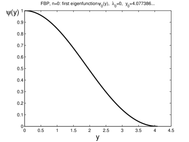
Figure 15. The first positive eigenfunction of (9.6), with the interface at $y_{0}^{(1)}=4.077386...\,$.

(a) four eigenfunctions

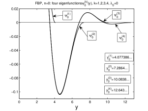
(b) enlarged zeros

Figure 16. First four eigenfunction of (9.6).

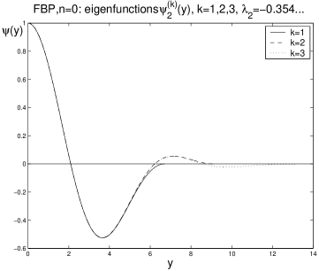
(a) four eigenfunctions

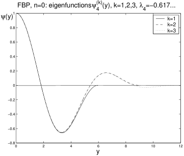
(b) enlarged zeros

Figure 17. First three profiles for the second and third even eigenfunctions $m=2,4$ of (9.11).

9.3. Nonlinear “Hermitian spectral theory”

Consider now the nonlinear eigenvalue problem (9.3) for $\lambda_{0}=0$ in the setting as in (9.6),

(9.12) $$\alpha=\frac{1}{4+n}\quad\Longrightarrow\quad-|f|^{n}f^{\prime\prime\prime}+\frac{1}{4+n}\,yf=0,\quad f=f^{\prime}=0\,\,\,\mbox{at the interfaces}.$$

Obviously, the first eigenfunction $\psi_{0}^{(1)}$ is positive and is the classic one first obtained in [5] (see also [13] for $N>1$). However, we claim that, similarly to Proposition 9.1, the following holds:

Conjecture 9.2. Besides the positive solution [5, 13], in the oscillatory range $n<n_{\rm h}$ given in $(\ref{n**1})$, the problem $(\ref{.10})$ admits a countable set of sign changing patterns $f^{(k)}=\psi_{0}^{(k)}(y)$, $k=1,2,...\,$, where each $k$-th one has precisely $k$ zeros for $y\in(0,y_{0}^{(k)}]$.

A rigorous proof is still incomplete since it requires detailed knowledge of oscillatory structures near interfaces such as (3.5). This should play a similar role to the linear expansion as in (9.9). Such a deep understanding of the nonlinear expansion is still not achieved.

In Figure 18, we show the first two eigenfunctions of the problem (9.12) for $n=1$. It is difficult to demonstrate more functions, since the next ones are already very close to the Cauchy profile denoted by $\psi_{0}^{(\infty)}$. The oscillations of this CP-profile $F(y)$ are presented in Figure 19, in between of the humps of which the interfaces of further nonlinear eigenfunction $\psi_{0}^{(k)}(y)$ are assumed to be situated.

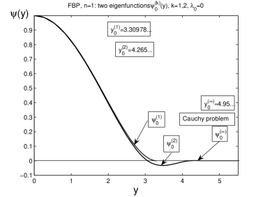
Figure 18. Two nonlinear eigenfunctions of (9.12) for $n=1$.

(a) $\sim 10^{-3}$

(b) $\sim 10^{-6}$

Figure 19. The CP-eigenfunction of (9.12), with $n=1$, for $k=\infty$, with the interface at $y_{0}^{(\infty)}=4.95...\,$.

For $\lambda\neq 0$, the corresponding statement to (9.12) is

(9.13) $$\left\{\begin{matrix}-|f|^{n}f^{\prime\prime\prime}+\frac{1+n\lambda}{n+4}\,yf=\lambda\int\limits_{0}^{y}f(s)\,{\mathrm{d}}s\,\,\,\mbox{on}\,\,\,(0,y_{+}),\qquad\qquad\,\,\,\,\,\vskip 3.0pt plus 1.0pt minus 1.0pt\\ f(0)=1,\,\,\,f^{\prime}(0)=0;\quad f(y_{+})=f^{\prime}(y_{+})=|f|^{n}f^{\prime\prime\prime}(y_{+})=0,\end{matrix}\right.$$

with $\lambda=\frac{1-\alpha(n+4)}{4}$. Again the sets of even eigenfunctions are denoted by $\{f=\psi_{m},\lambda=\lambda_{m},y_{+}=y_{m}\}$, using the subscript $m=0,2,4,\ldots$. Within each set (i.e. $m$ fixed), we have a countable set of eigenfunctions $\left\{\psi_{m}=\psi_{m}^{(k)},y_{m}=y_{m}^{(k)}\right\},k=1,2,3,...\,$. The first three eigenfunctions for the second $m=2$ and the fourth $m=4$ even sets are shown in Figure 20 for the case $n=1$. In the nonlinear case $n>0$, unlike the linear one $n=0$ above, convergence of numerical methods become much more slower.

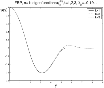
(a) four eigenfunctions

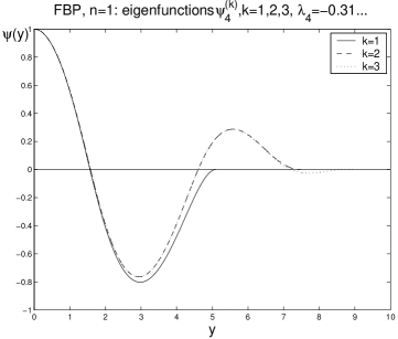
(b) enlarged zeros

Figure 20. The first three profiles for the second and third even eigenfunctions $m=2,4$ of (9.13) for $n=1$. These numerical solutions of (9.13) used the regularisation (3.12) with $\delta=0.1$.

9.4. Comments on $n$-branching and $p$-bifurcations

These properties are assumed to be similar to those developed earlier for the CP-setting. However, there are essential difficulties even in doing some formal computations.

Overall, we expect that the nonlinear eigenvalue problem (9.12) (see Conjecture 9.2) admits $n$-branching as $n\to 0^{+}$ from linear eigenfunctions from Proposition 9.1. As usual “variations” of the free boundary then must be taken into accound, which does not lead to any extra difficulty.

Furthermore, the general VSS problem (9.2) possesses $p$-bifurcation branches obtained via nonlinear bifurcations, whose theory is developed along the same lines used in Section 5.2. In particular, as in (5.9), the first bifurcation exponent will be

$$p_{0}(n)=\frac{n+2}{2}+\frac{1}{2\alpha_{0}(n)}\equiv\frac{n+2}{2}+\frac{n+4}{2}=n+3.$$

Similar to the analysis in Section 5.2, further study is necessary to check whether a “nonlinear bifurcation” occurs at $p=p_{0}$ (possibly not as for $n=0$), so further critical exponents $\alpha=\alpha_{l}(n)$ should be revealed.

We also expect that the above set of nonlinear eigenfunction-eigenvalue $\{f_{l}(y),\,\alpha_{l}(n)\}$ pairs for the CP for the TFE (1.9) also play a role for the FBP. More precisely, it is expected that, for any given CP profile $f_{l}(y)$, with $\alpha=\alpha_{l}(n)$, there exists a countable set of FBP profiles $\{f_{l}^{j}(y),\,\alpha_{l}(n)\}$, which are defined on the expanding intervals $[0,y_{l}^{j})$, where $y_{0}^{j}\to y_{0}^{(\infty)}$ (the interface of the CP-profile) as $j\to\infty$. Eventually, there holds:

(9.14) $$f_{l}^{j}(y)\to f_{l}(y)\quad\mbox{as}\quad j\to\infty$$

uniformly on compact subsets. In other words, each CP profile $f_{l}(y)$ can be arbitrarily closely approximated by FBP ones with a finite number of sign changes. The convergence (9.14) is a difficult open problem, both analytically and numerically even for the first values of $l$. Of course, (9.14) is associated with the discovered oscillatory properties of all the VSS CP profiles.

Again, we mention that the FBP problems have a different nature and are more difficult than the CP, since a new free parameter the interface location $y_{0}>0$ (an extra “nonlinear eigenvalue”) appears in the mathematical setting.

10. Discussion

We began in Section 2 with the similarity analysis of global, source-type (for $p=p_{0}$) and very singular (for $p\not=p_{0}$) solutions of the TFE with a stable parabolic term (1.1). Treating the Cauchy problem (respectively, the FBP), we first described in Section 3 for the CP (respectively, 7 for the FBP) the local asymptotic properties of solutions near interfaces. While the FBP asymptotics turned out to be standard and reasonably well known since the 1990s, it is important that, for the CP, we detected the nonlinearity range $n\in(0,n_{\rm h})$ ($n_{\rm h}$ is the point of a heteroclinic bifurcation for a nonlinear related ODE), in which the rescaled ODE exhibits a unique stable periodic motion describing, as expected, generic changing sign properties of more general solutions.

In Section 3, we studied the CP in the critical case

$$p=p_{0}=n+1+\frac{2}{N},$$

where we detected continuous branches of similarity profiles. In Section 4, we developed $n$-branching theory of similarity solutions of the 1D pure TFE

$$u_{t}=-(|u|^{n}u_{xxx})_{x},$$

where we described branching of nonlinear similarity profiles from eigenfunctions of a linear rescaled operator at $n=0$. This allowed us in Section 5 to reveal a countable sequence of critical exponents $\{p_{l}\}$ of the original stable TFE (1.1) and to describe similarity solutions for $p\not=p_{0}$.

After a detailed study of the CP, we returned to the FBP setting. We studied in Section 8 various branches of similarity patterns for the FBP in the critical case $p=p_{0}$ and extended some of the results to $p\not=p_{0}$ in Section 9.

By comparing the similarity patterns of the CP and the FBP, a striking “limit” property emerges: the infinitely oscillatory patterns of the CP are the limits of FBP-patterns with a finite number of sign changes. Naturally, this is required to take into account sign changing patterns of the FBP, which have not been previously studied in any detail. In a sense, the above limit property can be considered as a certain definition of solutions of the CP (besides the already existing ones via maximal regularity at the interfaces or via a smooth analytic “homotopy” deformation to the bi-harmonic equation $u_{t}=-\Delta^{2}u$, which turned out to be a good approximation of the TFE for small $n>0$; [10]).

Thus, the goal of the paper was to describe some leading key ideas concerning (i) formation of similarity solutions for the stable TFEs and (ii) extra relations between the CP and the FBP. Some of the most difficult conclusions remain formal, the related mathematics turns out to be very difficult, and we have posed several open problems for future research.

References

- [1] F. Bernis, Source-type solutions of fourth order degenerate parabolic equations, In: Proc. Microprogram Nonlinear Diffusion Eqs Equilibrium States, W.-M. Ni, L.A. Peletier, and J. Serrin, Eds., MSRI Publ., Berkeley, California, Vol. 1, New York, 1988, pp. 123–146.
- [2] F. Bernis and A. Friedman, Higher order nonlinear degenerate parabolic equations, J. Differ. Equat., 83 (1990), 179–206.
- [3] F. Bernis, J. Hulshof, and J.R. King, Dipols and similarity solutions of the thin film equation in the half-line, Nonlinearity, 13 (2000), 413–439.
- [4] F. Bernis and J.B. McLeod, Similarity solutions of a higher order nonlinear diffusion equation, Nonl. Anal., 17 (1991), 1039–1068.
- [5] F. Bernis, L.A. Peletier, and S.M. Williams, Source type solutions of a fourth order nonlinear degenerate parabolic equation, Nonl. Anal., TMA, 18 (1992), 217–234.
- [6] M. Bowen, J. Hulshof, and J.R. King, Anomalous exponents and dipole solutions for the thin film equation, SIAM J. Appl. Math., 62 (2001), 149–179.
- [7] M. Bowen and T.P. Witelski, The linear limit of the dipole problem for the thin film equation, SIAM J. Appl. Math., 66 (2006), 1727–1748.
- [8] Yu.V. Egorov, V.A. Galaktionov, V.A. Kondratiev, and S.I. Pohozaev, Asymptotic behaviour of global solutions to higher-order semilinear parabolic equations in the supercritical range, Adv. Differ. Equat., 9 (2004), 1009–1038.
- [9] J.D. Evans, V.A. Galaktionov, and J.R. King, Blow-up similarity solutions of the fourth-order unstable thin film equation, Euro J. Appl. Math., 18 (2007), 195–231.
- [10] J.D. Evans, V.A. Galaktionov, and J.R. King, Source-type solutions for the fourth-order unstable thin film equation, Euro J. Appl. Math., 18 (2007), 273–321.
- [11] J.D. Evans, V.A. Galaktionov, and J.R. King, Unstable sixth-order thin film equation I. Blow-up similarity solutions; II. Global similarity patterns, Nonlinearity, 20 (2007), 1799–1841, 1843–1881.
- [12] J.D. Evans, V.A. Galaktionov, and J.F. Williams, Blow-up and global asymptotics of the limit unstable Cahn-Hilliard equation, SIAM J. Math. Anal., 38 (2006), 64–102.
- [13] R. Ferreira and F. Bernis, Source-type solutions to thin-film equations in higher dimensions, Euro J. Appl. Math., 8 (1997), 507–534.
- [14] V.A. Galaktionov, Evolution completeness of separable solutions of non-linear diffusion equations in bounded domains, Math. Meth. Appl. Sci., 27 (2004), 1755–1770.
- [15] V.A. Galaktionov, Sturmian nodal set analysis for higher-order parabolic equations and applications, Adv. Differ. Equat., 12 (2007), 669–720.
- [16] V.A. Galaktionov and P.J. Harwin, On evolution completeness of nonlinear eigenfunctions for the porous medium equation in the whole space, Adv. Differ. Equat., 10 (2005), 635–674.
- [17] V.A. Galaktionov and P.J. Harwin, On centre subspace behaviour in thin film equations, SIAM J. Appl. Math., 69 (2009), 1334–1358 (an earlier preprint in arXiv:0901.3995v1).
- [18] V.A. Galaktionov and S.R. Svirshchevskii, Exact Solutions and Invariant Subspaces of Nonlinear Partial Differential Equations in Mechanics and Physics, ChapmanHall/CRC, Boca Raton, Florida, 2007.
- [19] V.A. Galaktionov and J.F. Williams, On very singular similarity solutions of a higher-order semilinear parabolic equation, Nonlinearity, 17 (2004), 1075–1099.
- [20] I. Gohberg, S. Goldberg, and M.A. Kaashoek, Classes of Linear Operators, Vol. 1, Operator Theory: Advances and Applications, Vol. 49, Birkhäuser Verlag, Basel/Berlin, 1990.
- [21] J. Hulshof, Similarity solutions of the porous medium equation with sign changes, J. Math. Anal. Appl., 157 (1991), 75-111.
- [22] A.N. Kolmogorov and S.V. Fomin, Elements of the Theory of Functions and Functional Analysis, Nauka, Moscow, 1976.
- [23] M.A. Krasnosel’skii and P.P. Zabreiko, Geometrical Methods of Nonlinear Analysis, Springer-Verlag, Berlin/Tokyo, 1984.
- [24] L. Perko, Differential Equations and Dynamical Systems, Springer-Verlag, New York, 1991.
- [25] M.A. Vainberg and V.A. Trenogin, Theory of Branching of Solutions of Non-Linear Equations, Noordhoff Int. Publ., Leiden, 1974.
- [26] Z. Wu, J. Zhao, J. Yin, and H. Li, Nonlinear Diffusion Equations, World Scientific Publ. Co., Inc., River Edge, NJ, 2001.
- [27] Ya.B. Zel’dovich, The motion of a gas under the action of a short term pressure shock, Akust. Zh., 2 (1956), 28–38; Soviet Phys. Acoustics, 2 (1956), 25–35.