A new structure for analyzing discrete scale
invariant processes: Covariance and Spectra

Abstract

Improving the efficiency of discrete time scale invariant (DSI) processes, we consider some flexible sampling of a continuous time DSI process $\{X(t),t\in{\bf R^{+}}\}$ with scale $l>1$, which is in correspondence to some multi-dimensional self-similar process. So we consider $q$ samples at arbitrary points ${\bf s}_{0},{\bf s}_{1},\ldots,{\bf s}_{q-1}$ in interval $[1,l)$ and proceed in the intervals $[l^{n},l^{n+1})$ at points $l^{n}{\bf s}_{0},l^{n}{\bf s}_{1},\ldots,l^{n}{\bf s}_{q-1}$, $n\in{\bf Z}$. So we study an embedded DT-SI process $W(nq+k)=X(l^{n}{\bf s}_{k})$, $q\in{\bf N}$, $k=0,\ldots,q-1$, and its multi-dimensional self-similar counter part $V(n)=\big{(}V^{0}(n),\ldots,V^{q-1}(n)\big{)}$ where $V^{k}(n)=W(nq+k)$. We study spectral representation of such process and obtain its spectral density matrix. Finally by imposing wide sense Markov property on $W(\cdot)$ and $V(\cdot)$, we show that the spectral density matrix of $V(\cdot)$ can be characterized by $\{R_{j}(1),R_{j}(0),j=0,\ldots,q-1\}$ where $R_{j}(k)=E[W(j+k)W(j)]$.

AMS 2010 Subject Classification: 60G18, 62M15, 60J05.

Keywords: Discrete scale invariance; Wide sense Markov; Multi-dimensional self-similar process; Spectral density matrix; Brownian motion.

1 Introduction

The concept of stationarity and self-similarity are used as a fundamental property to handle many natural phenomena. Lamperti transformation defines a one to one correspondence between stationary and self-similar processes. Discrete scale invariant (DSI) processes can be defined as the Lamperti transform of periodically correlated ones. Many critical systems, like statistical physics, textures in geophysics, network traffic and image processing can be interpreted by these processes [1]. Fourier transform is known as a suited representation for stationary processes. Using Mellin transform, a harmonic like representation of self-similar process is introduced [4]. Self-similar Markov process which has Markov property and self-similarity are involved in various parts of probability theory, such as branching processes and fragmentation theory [2]. Gladyshev in [5] introduced the spectral representation of correlation matrix of multi-dimensional stationary random sequences and found a relation between them and periodically correlated (PC) processes.

In our previous work [6] we studied spectral analysis of a sequence of observations which are sampled at some special points, $\alpha^{k}$, $k\in{\mathbb{Z}}$ of a DSI process with some scale $l=\alpha^{T}$, $T\in{\mathbb{N}}$. So that one could study such processes in spectral domain. By such sampling, and by imposing wide sense Markov property, we provided a discrete time scale invariant sequence which is Markov in the wide sense and found a closed formula for its covariance function and spectral density matrix of corresponding multi-dimensional self-similar process. The above sampling scheme had much restrictions which could dismiss lots of information between sample points $\alpha^{k}$. In this paper we consider some flexible sampling scheme which enables one to have samples at arbitrary points ${\bf s}_{0},{\bf s}_{1},\ldots,{\bf s}_{q-1}$ in the first scale interval and follow sampling at corresponding points $\{l^{n}{\bf s}_{i},n\in\mathbb{N},i=0,\ldots,q-1\}$ in the other scale intervals. This sampling scheme provide a corresponding multi-dimensional self-similar process as a platform to extend analytic property of discrete time periodically correlated Markov process to such DSI sequences. For such study we need to consider a new approach for modeling this sequence via defining some embedded process. So this method enables one to study the behavior of the process specially in spectral domain and have a better description of the underlying DSI process at all arbitrary points.

Let $X(\cdot)$ be a DSI process with scale $l>1$. By sampling at arbitrary points in the scale intervals $[l^{n-1},l^{n})$, $n\in{\mathbb{N}}$, we provide $\{X(l^{n-1}{\bf s}_{k}),n\in{\mathbb{N}};1\leq{\bf s}_{0}<\cdots<{\bf s}_{q-1}<l\}$ as a sequence of DSI. Then we define an embedded scale invariant process as $\{W(nq+k)\equiv X(l^{n}{\bf s}_{k});n\in{\mathbb{W}},k=0,\ldots,q-1\}$ where $\mathbb{W}=\{0,1,\ldots\}$ and its corresponding multi-dimensional embedded self-similar process as $\{V(n),n\in{\mathbb{W}}\}$, where $V(n)=\big{(}V^{0}(n),\ldots,V^{q-1}(n)\big{)}$, and $\{V^{i}(n)\equiv W(nq+i),n\in{\mathbb{W}},i=0,\ldots,q-1\}$, for fixed $q\in{\mathbb{N}}$. We investigate covariance structure and spectral density matrix of $\{U(l^{n}),n\in{\mathbb{W}}\}$, where $U(l^{n})=\big{(}U^{0}(l^{n}),\ldots,U^{q-1}(l^{n})\big{)}$, and $\{U^{i}(l^{n})\equiv X(l^{n}{\bf s}_{i}),n\in{\mathbb{W}},i=0,\ldots,q-1\}$, for fixed $q\in{\mathbb{N}}$, when it is Markov in the wide sense and is called multi-dimensional self-similar Markov process.

This paper is organized as follows. In section 2, we present multi-dimensional stationary, PC, self-similar and DSI processes and define them in discrete time. We also review the properties of Lamperti transformation in this section. Section 3 is devoted to the structure of the multi-dimensional self-similar process resulting from the above method of sampling. We define embedded scale invariant process and corresponding multi-dimensional embedded self-similar process and characterize the spectral density matrix of it in this section. We also characterize covariance function and spectral density matrix of the multi-dimensional self-similar and embedded self-similar Markov processes in section 4 which is characterized by $\{R_{j}(1),R_{j}(0),j=0,\ldots,q-1\}$ where $R_{j}(k)=E[W(j+k)W(j)]$. We simulate and analyze Simple Brownian Motion (SBM) as a DSI Markov and its corresponding multi-dimensional processes. Throughout this paper we study above mentioned processes in the discrete time with some clarified parameter spaces. So we omit the term discrete time in the rest of this paper.

2 Theoretical framework

In this section we review the structure of covariance function and spectral density matrix of multi-dimensional stationary processes. The definitions of self-similar, scale invariant processes in discrete time and in the wide sense are presented. Also Lamperti transformation is defined and its properties are studied.

2.1 Stationary and multi-dimensional stationary processes

Definition 2.1

A process $\{Y(t),t\in{\mathbb{R}}\}$ is said to be stationary, if for any $\tau\in{\mathbb{R}}$

$$\{Y(t+\tau),t\in{\mathbb{R}}\}\stackrel{{\scriptstyle d}}{{=}}\{Y(t),t\in{\mathbb{R}}\}$$ (2.1)

where $\stackrel{{\scriptstyle d}}{{=}}$ is the equality of all finite-dimensional distributions.

If $(2.1)$ holds for some $\tau\in{\mathbb{R}}$, the process is said to be periodically correlated. The smallest of such $\tau$ is called period of the process.

By Rozanov [7], if $Y(t)=\{Y^{k}(t)\}_{k=1,\ldots,n}$ be an $n$-dimensional stationary process, then

$$Y(t)=\int e^{i\lambda t}\phi(d\lambda)$$ (2.2)

is its spectral representation, where $\phi=\{\varphi_{k}\}_{k=1,\ldots,n}$ and $\varphi_{k}$ is the random spectral measure associated with the $k$th component $Y^{k}$ of the $n$-dimensional process $Y$. Let

$$B_{kr}(\tau)=E[Y^{k}(\tau+t)\overline{Y^{r}(t)}],\hskip 19.91692ptk,r=1,\ldots,n$$

and $B(\tau)=[B_{kr}(\tau)]_{k,r=1,\ldots,n}$ be the correlation matrix of $Y$. The components of the correlation matrix of the process $Y$ can be represented as

$$B_{kr}(\tau)=\int e^{i\lambda\tau}F_{kr}(d\lambda),\hskip 19.91692ptk,r=1,\ldots,n$$ (2.3)

where for any Borel set $\Delta$, $F_{kr}(\Delta)=E[\varphi_{k}(\Delta)\overline{\varphi_{r}(\Delta)}]$ are the complex valued set functions which are $\sigma$-additive and have bounded variation. For any $k,r=1,\ldots,n$, if the sets $\Delta$ and $\Delta^{\prime}$ do not intersect, $E[\varphi_{k}(\Delta)\overline{\varphi_{r}(\Delta^{\prime})}]=0$. For any interval $\Delta=(\lambda_{1},\lambda_{2})$ when $F_{kr}(\{\lambda_{1}\})=F_{kr}(\{\lambda_{2}\})=0$ the following relation holds

$$F_{kr}(\Delta)=\frac{1}{2\pi}\int_{\Delta}\sum_{\tau=-\infty}^{\infty}B_{kr}(\tau)e^{-i\lambda\tau}d\lambda$$ (2.4)

$$=\frac{1}{2\pi}B_{kr}(0)[\lambda_{2}-\lambda_{1}]+\lim_{T\rightarrow\infty}\frac{1}{2\pi}\sum_{0<|\tau|\leqslant T}B_{kr}(\tau)\frac{e^{-i\lambda_{2}\tau}-e^{-i\lambda_{1}\tau}}{-i\tau}$$

in the discrete parameter case, and

$$F_{kr}(\Delta)=\lim_{a\rightarrow\infty}\frac{1}{2\pi}\int_{-a}^{a}\frac{e^{-i\lambda_{2}\tau}-e^{-i\lambda_{1}\tau}}{-i\tau}B_{kr}(\tau)d\tau$$

in the continuous parameter case.

2.2 Discrete time scale invariant processes

Definition 2.2

A process $\{X(t),t\in{\mathbb{R}^{+}}\}$ is said to be self-similar of index $H>0$, if for any ${\lambda}>0$

$$\{\lambda^{-H}X(\lambda t),t\in{\mathbb{R}}\}\stackrel{{\scriptstyle d}}{{=}}\{X(t),t\in{\mathbb{R}}\}.$$ (2.5)

The process is said to be DSI of index $H$ and scaling factor ${\lambda}_{0}>0$ or (H,${\lambda}_{0}$)-DSI, if $(2.5)$ holds for $\lambda=\lambda_{0}$.

As an intuition, self-similarity refers to an invariance with respect to any dilation factor. However, this may be a too strong requirement for capturing in situations that scaling properties are only observed for some preferred dilation factors.

Definition 2.3

A process $\{X(k),k\in{\hat{T}}\}$ is called discrete time self-similar process with parameter space $\hat{T}$, where $\hat{T}$ is any subset of countable distinct points of positive real numbers, if for any $k_{1},k_{2}\in\check{T}$

$$\{X(k_{2})\}\stackrel{{\scriptstyle d}}{{=}}(\frac{k_{2}}{k_{1}})^{H}\{X(k_{1})\}.$$ (2.6)

The process $X(\cdot)$ is called discrete time scale invariant with scale $l>0$ and parameter space $\hat{T}$, if for any $k_{1},k_{2}=lk_{1}\in\hat{T}$, $(2.6)$ holds.

Remark 2.1

If the process $\{X(t),t\in{\mathbb{R}^{+}}\}$ is DSI with scale $l>1$. Then by sampling of the process at points of set

$$\check{T}=\{l^{n}{\bf s}_{j},n\in{\mathbb{Z}},1\leq{\bf s}_{0}<\cdots<{\bf s}_{q-1}<l\}$$

for $j=0,\ldots,q-1$, we have $X(\cdot)$ as a scale invariant process with parameter space $\check{T}$ and scale $l$. If we consider sampling of $X(\cdot)$ at points

$$\tilde{T}=\{l^{n}{\bf s}_{j},n\in{\mathbb{Z}}\ \ \text{for fixed}\ \ 1\leq{\bf s}_{j}<l\},$$

then $X(\cdot)$ is a self-similar process with parameter space $\tilde{T}$.

Based on the definition of wide sense self-similar process presented in [8], we present the following definition.

Definition 2.4

A random process $\{X(k),k\in\hat{T}\}$ is called self-similar in the wide sense with index $H>0$ and with parameter space $\hat{T}$, where $\hat{T}$ is any subset of distinct countable points of positive real numbers, if for all $k,k_{1}\in\hat{T}$ and all $c>0$, where $ck,ck_{1}\in\hat{T}$

$(i)\,\,\ E[X^{2}(k)]<\infty$,

$(ii)\,\,E[X(ck)]=c^{H}E[X(k)]$,

$(iii)\,\,E[X(ck)X(ck_{1})]=c^{2H}E[X(k)X(k_{1})]$.

If the above conditions hold for some fixed $c=c_{0}$, then the process is called scale invariant in the wide sense with scale $c_{0}$.

Throughout this paper we are dealt with wide sense self-similar and wide sense scale invariant process, and for simplicity we omit the term ”in the wide sense” hereafter.

2.3 Lamperti transformation

The Lamperti transformation provides a bijection between self-similar and stationary processes and also scale invariant and periodically correlated processes in discrete time.

Definition 2.5

The Lamperti transform with positive index $H$, denoted by ${\cal L}_{H}$ operates on a random process $\{Y(t),t\in{\mathbb{R}}\}$ as

$${\cal L}_{H}Y(t)=t^{H}Y(\ln t)$$ (2.7)

and the corresponding inverse Lamperti transform ${\cal L}^{-1}_{H}$ on process $\{X(t),t\in{\mathbb{R}^{+}}\}$ acts as

$${\cal L}^{-1}_{H}X(t)=e^{-tH}X(e^{t}).$$ (2.8)

Remark 2.2

If $\{Y(t),t\in{\mathbb{R}}\}$ is stationary process, its Lamperti transform $\{{\cal L}_{H}Y(t),t\in{\mathbb{R}^{+}}\}$ is self-similar. Conversely if $\{X(t),t\in{\mathbb{R}^{+}}\}$ is self-similar process, its inverse Lamperti transform $\{{\cal L}^{-1}_{H}X(t),t\in{\mathbb{R}}\}$ is stationary.

Remark 2.3

If $\{X(t),t\in{\mathbb{R}^{+}}\}$ is $(H,e^{T}$)-DSI then ${\cal L}^{-1}_{H}X(t)=Y(t)$ is periodically correlated with period $T>0$. Conversely if $\{Y(t),t\in{\mathbb{R}}\}$ is periodically correlated with period $T$ then ${\cal L}_{H}Y(t)=X(t)$ is $(H,e^{T}$)-DSI.

Remark 2.4

If $X(\cdot)$ is a self-similar process with parameter space $\check{T}=\{l^{n}{\bf s}_{i},i=0,1,\ldots,q-1;n\in\mathbb{W}\}$, then its stationary counterpart $Y(\cdot)$ has parameter space $\tilde{T}=\{n\ln l+\ln{\bf s}_{i},i=0,1,\ldots,q-1;n\in\mathbb{W}\}$

$$X(l^{n}{\bf s}_{i})={\cal L}_{H}Y(l^{n}{\bf s}_{i})=(l^{n}{\bf s}_{i})^{H}Y(n\ln l+\ln{\bf s}_{i}).$$

Also it is clear by the following relation that if $X(\cdot)$ is a scale invariant process with scale $l$ and parameter space $\check{T}=\{l^{n}{\bf s}_{i},i=0,1,\ldots,q-1;n\in\mathbb{W}\}$, then $Y(\cdot)$ is a discrete time periodically correlated process with period $q$ and parameter space $\tilde{T}=\{n\ln l+\ln{\bf s}_{i},i=0,1,\ldots,q-1;n\in\mathbb{W}\}$

$$Y(n\ln l+\ln{\bf s}_{i})={\cal L}^{-1}_{H}X(n\ln l+\ln{\bf s}_{i})=(l^{n}{\bf s}_{i})^{-H}X(l^{n}{\bf s}_{i}).$$

3 Structure of the process

In this section we introduce a new method for flexible sampling of a DSI process with scale $l>1$, which provide sampling at arbitrary points in the interval $[1,l)$ and at multiple $l^{n}$ of such points in the intervals $[l^{n},l^{n+1})$, $n\in{\mathbb{N}}$. Based on such a sequence of DSI process we define an embedded scale invariant process which follow this sequence. Then by introducing the corresponding multi-dimensional embedded self-similar process in the wide sense we provide a platform to characterize spectral representation and spectral density of the process. Finally in Theorem 3.1 we find harmonic like representation and spectral density matrix of the multi-dimensional embedded self-similar process.

Definition 3.1

The process $U(t)=(U^{0}(t),U^{1}(t),\ldots,U^{q-1}(t))$ with parameter space $\check{T}=\{l^{n},n\in{\mathbb{Z}}\}$ is a multi-dimensional self-similar process, where

$\bf(a)$    $\{U^{j}(\cdot)\}$ for every $j=0,1,\cdots,q-1$ is self-similar process with parameter space

$\check{T}=\{l^{n},n\in{\mathbb{Z}}\}$.

$\bf(b)$    For every $n,\tau\in{\mathbb{Z}},\,\ j,k=0,1,\cdots,q-1$

$$\mathrm{Cov}\big{(}U^{j}(l^{n+\tau}),U^{k}(l^{n})\big{)}=l^{2nH}\mathrm{Cov}\big{(}U^{j}(l^{\tau}),U^{k}(1)\big{)}.$$

Remark 3.1

Let $\{X(t),t\in\check{T}\}$ be a DSI process with scale $l>1$ and parameter space $\check{T}$, as defined in Remark 2.1. Then by definition $3.1$ we have that $\{U^{j}(l^{n})\equiv X(l^{n}{\bf s}_{j})\}$ for fixed $j=0,\ldots,q-1$, is a self-similar process and $U(l^{n})=\big{(}X(l^{n}{\bf s}_{0}),\ldots,X(l^{n}{\bf s}_{q-1})\big{)}$ where $1\leq{\bf s}_{0}<\cdots<{\bf s}_{q-1}<l$ is a multi-dimensional self-similar process.

By such method of sampling at discrete points, we provide a $q$-dimensional embedded self-similar process $V(n)$ as

$$V(n)=\big{(}V^{0}(n),V^{1}(n),\ldots,V^{q-1}(n)\big{)},\hskip 28.45274ptn\in{\mathbb{Z}}$$

where $\{V^{u}(n)\equiv X(l^{n}{\bf s}_{u})\}$ and $\{V(n)\equiv U(l^{n})\}$ in which $U(l^{n})$ and ${\bf s}_{u}$ follows the same assumptions as in Remark 3.1. Such definition of multi-dimensional embedded self-similar provides a platform to obtain spectral density of $U(l^{n})$ in the followings.

Remark 3.2

Corresponding to the $q$-dimensional embedded self-similar process $V(n)$ there exists an embedded scale invariant process $\big{\{}W(\kappa),\kappa\in{\mathbb{Z}}\big{\}}$ with scale $l$ as

$$\{W(\kappa)\equiv X(l^{n}{\bf s}_{u})\}\hskip 28.45274pt\kappa\in{\mathbb{Z}}$$ (3.1)

where $u=\kappa-q[\frac{\kappa}{q}]$, $n=[\frac{\kappa}{q}]$ and $\kappa=nq+u$, where by $(3.1)$

$$W(\kappa+q)\equiv X(l^{(n+1)}{\bf s}_{u})\stackrel{{\scriptstyle d}}{{=}}l^{H}X(l^{n}{\bf s}_{u})\equiv l^{H}W(\kappa).$$

So the scale invariant process $\big{\{}X(l^{n}{\bf s}_{u}),1\leq{\bf s}_{0}<\cdots<{\bf s}_{q-1};n\in{\mathbb{Z}}\big{\}}$ and the embedded scale invariant process $\big{\{}W(\kappa),\kappa\in{\mathbb{Z}}\big{\}}$, can be considered as counterparts.

By the following theorem, the spectral representation and spectral density matrix of the $q$-dimensional embedded self-similar process and harmonic like representation of each column is obtained.

Theorem 3.1

Let $X(\cdot)$ be a DSI process with scale $l$ and $1\leqslant{\bf s}_{0}<\ldots<{\bf s}_{q-1}<l$, then $V(n)=\big{(}V^{0}(n),\ldots,V^{q-1}(n)\big{)}$, where $\{V^{u}(n)\equiv X(l^{n}{\bf s}_{u})\}$, $n\in{\mathbb{Z}}$ and $u=0,\ldots,q-1$ is a multi-dimensional embedded self-similar process and

(i) Harmonic like representation of $V^{u}(n)$ for fixed $u$ and $n\in{\mathbb{Z}}$ is

$$V^{u}(n)=(l^{n}{\bf s}_{u})^{H}\int_{0}^{2\pi}e^{i\omega n}d\phi_{u}(\omega)$$ (3.2)

where $\{\phi_{u}(\omega)\}$ are orthogonal spectral measures. $E[d\phi_{u}(\omega)\overline{d\phi_{\nu}(\omega^{\prime})}]=dG_{u,v}^{H}(\omega)$ when $\omega=\omega^{\prime}$, and is zero when $\omega\neq\omega^{\prime}$ for $u,\nu=0,\ldots,q-1$.

(ii) Spectral density matrix of $\{V(n)\equiv U(l^{n})\}$ is $g^{H}(\omega)=[g_{u,\nu}^{H}(\omega)]_{u,\nu=0,\ldots,q-1},$ where the elements $g_{u,v}^{H}(\omega)=dG_{u,v}^{H}(\omega)/d\omega$ are

$$g_{u,\nu}^{H}(\omega)=\frac{({\bf s}_{u}{\bf s}_{\nu})^{-H}}{2\pi}\sum_{\tau=-\infty}^{\infty}l^{-H\tau}e^{-i\omega\tau}Q^{H}_{u,\nu}(\tau)$$ (3.3)

$\tau\in{\mathbb{N}}$ and $Q^{H}_{u,\nu}(\tau)$ is the covariance function of $V^{u}(\tau)$ and $V^{\nu}(0)$.

Proof of (i): Remark $2.4$ implies that

$$V^{u}(n)\equiv X(l^{n}{\bf s}_{u})={\cal L}_{H}Y(l^{n}{\bf s}_{u})=(l^{n}{\bf s}_{u})^{H}\eta^{u}(n)$$

where $\eta^{u}(n)=Y(n\ln l+\ln{\bf s}_{u})$. Thus $V^{u}(n)$ for every $u=0,1,\ldots,q-1$ is an embedded self-similar process in $n$, where its discrete time stationary counterpart $\eta^{u}(n)$ for fixed $u=0,1,\ldots,q-1$ has spectral representation $\eta^{u}(n)=\int_{0}^{2\pi}e^{i\omega n}d\phi_{u}(\omega)$.

Proof of (ii): The covariance matrix of $V(n)$ is denoted by $Q^{H}(n,\tau)=[Q^{H}_{u,\nu}(n,\tau)]_{u,\nu=0,\ldots,q-1}$ where

$$Q^{H}_{u,\nu}(n,\tau)=E[V^{u}(n+\tau)V^{\nu}(n)]=E[X(l^{(n+\tau)}{\bf s}_{u})X(l^{n}{\bf s}_{\nu})]$$

By the scale invariant property of the process $X(\cdot)$ we have that

$$Q^{H}_{u,\nu}(n,\tau)=l^{2nH}E[X(l^{\tau}{\bf s}_{u})X({\bf s}_{\nu})]=l^{2nH}Q^{H}_{u,\nu}(\tau)$$ (3.4)

where $Q^{H}_{u,\nu}(\tau)=Q^{H}_{u,\nu}(0,\tau)=E[V^{u}(\tau)\overline{V^{\nu}(0)}]$, then by (3.2)

$$Q^{H}_{u,\nu}(\tau)=E[(l^{\tau}{\bf s}_{u})^{H}({\bf s}_{\nu})^{H}\int_{0}^{2\pi}e^{i\omega\tau}d\phi_{u}(\omega)\int_{0}^{2\pi}\overline{d\phi_{v}(\omega^{\prime})}]$$

$$=l^{\tau H}({\bf s}_{u}{\bf s}_{\nu})^{H}\int_{0}^{2\pi}e^{i\omega\tau}dG^{H}_{u,\nu}(\omega)$$ (3.5)

where $E[d\phi_{u}(\omega)\overline{d\phi_{\nu}(\omega^{\prime})}]=dG^{H}_{u,\nu}(\omega)$ when $\omega=\omega^{\prime}$ and is $0$ when $\omega\neq\omega^{\prime}$.
On the other hand, by the definition of $\eta^{u}(n)$ in the proof of part $(i)$

$$Q^{H}_{u,\nu}(\tau)=E[X(l^{\tau}{\bf s}_{u})X({\bf s}_{\nu})]=E[{\cal L}_{H}Y(l^{\tau}{\bf s}_{u}){\cal L}_{H}Y({\bf s}_{\nu})]$$

$$=(l^{\tau}{\bf s}_{u}{\bf s}_{\nu})^{H}E[Y(\tau\ln l+\ln{\bf s}_{u})Y(\ln{\bf s}_{\nu})]$$

$$=(l^{\tau}{\bf s}_{u}{\bf s}_{\nu})^{H}E[\eta^{u}(\tau)\eta^{\nu}(0)]=(l^{\tau}{\bf s}_{u}{\bf s}_{\nu})^{H}B_{u,\nu}(\tau).$$

As $\eta^{u}(\cdot)$ ia a stationary process so by (2.3)

$$B_{u,\nu}(\tau)=\int_{0}^{2\pi}e^{i\omega\tau}dG^{H}_{u,\nu}(\omega),\hskip 14.22636ptu,\nu=0,\ldots,q-1$$

Now by (2.4) for $u,\nu=0,\ldots,q-1$ we have

$$G^{H}_{u,\nu}(A)=\frac{1}{2\pi}\int_{A}\sum_{\tau=-\infty}^{\infty}B_{u,\nu}(\tau)e^{-i\lambda\tau}d\lambda.$$

By substituting $B_{u,\nu}(\tau)=(l^{\tau}{\bf s}_{u}{\bf s}_{\nu})^{-H}Q^{H}_{u,\nu}(\tau)$, the elements of the spectral distribution function, $G^{H}_{u,\nu}(\cdot)$ has the following representation

$$G^{H}_{u,\nu}(A)=\frac{({\bf s}_{u}{\bf s}_{\nu})^{-H}}{2\pi}\int_{A}\sum_{\tau=-\infty}^{\infty}l^{-H\tau}e^{-i\lambda\tau}Q^{H}_{u,\nu}(\tau)d\lambda.$$ (3.6)

Let $A=(\omega,\omega+d\omega]$, then the elements of the spectral density matrix, $g_{u,\nu}^{H}(\omega)$ are

$$g_{u,\nu}^{H}(\omega):=\frac{G^{H}_{u,\nu}(d\omega)}{d\omega}=\frac{({\bf s}_{u}{\bf s}_{\nu})^{-H}}{2\pi}\sum_{\tau=-\infty}^{\infty}l^{-H\tau}\big{(}\frac{1}{d\omega}\int_{\omega}^{\omega+d\omega}e^{-i\lambda\tau}d\lambda\big{)}Q^{H}_{u,\nu}(\tau)$$

$$=\frac{({\bf s}_{u}{\bf s}_{\nu})^{-H}}{2\pi}\sum_{\tau=-\infty}^{\infty}l^{-H\tau}\big{(}\frac{1}{-i\tau}\lim_{d\omega\rightarrow 0}\frac{e^{-i{(\omega+d\omega)\tau}}-e^{-i\omega\tau}}{d\omega}\big{)}Q^{H}_{u,\nu}(\tau).$$

Thus we get to the assertion of part (ii) of the theorem.$\square$

4 Scale invariant process with Markov property

Using the method of sampling in section 3 and the scale invariant process $X(\cdot)$ in Remark 3.1, and its corresponding embedded scale invariant process $W(\cdot)$ in Remark 3.2, we introduce $W(\cdot)$ with Markov property in the wide sense, named embedded scale invariant Markov process. Also the corresponding multi-dimensional embedded self-similar process $V(\cdot)$ and its corresponding multi-dimensional self-similar process $U(\cdot)$ is defined. We find the covariance function of embedded scale invariant Markov process in subsection 4.1. The spectral density matrix of multi-dimensional process of it embedded is evaluated in subsection 4.2.

4.1 Covariance function of embedded scale invariant Markov process

Here we characterize the covariance function of the embedded scale invariant Markov process $\{W(\kappa),\kappa\in{\mathbb{Z}}\}$ in Theorem 4.1 and the covariance function of the associated multi-dimensional embedded self-similar Markov process in Theorem 4.2.

Theorem 4.1

Let $\{W(\kappa),\kappa\in{\mathbb{Z}}\}$, defined by $(3.1)$, be an embedded scale invariant and Markov process in the wide sense with scale $l$. Then for $\tau\in{\mathbb{W}}$, $\kappa=nq+\nu$, $\kappa+\tau=mq+u$, $u,\nu=0,\ldots,q-1$ and $n,m\in{\mathbb{Z}}$, the covariance function

$$R_{\kappa}(\tau):=E[W(\kappa+\tau)W(\kappa)]=E[X(l^{m}{\bf s}_{u})X(l^{n}{\bf s}_{\nu})]$$ (4.1)

where $1\leqslant{\bf s}_{0}<{\bf s}_{1}<\ldots<{\bf s}_{q-1}<l$, can be characterized as

$$R_{\kappa}(tq+w)=[\tilde{f}(q-1)]^{t}\tilde{f}(\kappa+w-1)[\tilde{f}(\kappa-1)]^{-1}R_{\kappa}(0),$$ (4.2)

$t\in{\mathbb{Z}}$, $w=0,\ldots,q-1$

$$\tilde{f}(r)=\prod_{j=0}^{r}f(j)=\prod_{j=0}^{r}R_{j}(1)/R_{j}(0),\hskip 19.91692ptr\in{\mathbb{Z}},\tilde{f}(-1)=1.$$ (4.3)

Proof: By considering sample points of this paper, proof of this theorem follows by a similar method as for theorem 3.2 of [6].

Now we can use this theorem to prove the next result for multi-dimensional embedded self-similar Markov process.

Theorem 4.2

Let $\{W(\kappa),\kappa\in{\mathbb{Z}}\}$ be a embedded scale invariant Markov process, and $\{V(n)\equiv U(l^{n})\}$ be its associated multi-dimensional embedded self-similar Markov, where $\{U(l^{n}),n\in{\mathbb{Z}}\}$ is the corresponding self-similar Markov process, both with the same covariance matrix $Q^{H}(n,\tau)$ which is defined by $(3.5)$. Then

$$Q^{H}(n,\tau)=l^{2nH}[\tilde{f}(q-1)]^{\tau}CD,\hskip 19.91692pt\tau\in{\mathbb{Z}}$$ (4.4)

where $\tilde{f}(\cdot)$ is defined in $(4.3)$ and the matrices $C$ and $D$ are given by $C=[C_{u,\nu}]_{u,\nu=0,\ldots,q-1}$, where $C_{u,\nu}=\tilde{f}(u-1)[\tilde{f}(\nu-1)]^{-1}$, and $D$ is a diagonal matrix with diagonal elements $R_{\nu}(0)$, $\nu=0,1,\ldots,q-1$, which is defined in $(4.1)$.

Proof: As $W(\cdot)$ is embedded scale invariant with scale $l$, (3.2) and (3.5) indicate that $Q^{H}_{u,\nu}(n,\tau)=l^{2nH}Q^{H}_{u,\nu}(\tau)$. Now by the assumption $\kappa=nq+\nu$ and $\kappa+\tau=mq+u$ where $m,n\in{\mathbb{Z}}$, $\tau\in{\mathbb{W}}$, we have $\tau=(m-n)q+u-\nu$ and therefore

$$R_{\kappa}(\tau)=R_{nq+\nu}((m-n)q+u-\nu)=E[W(mq+u)W(nq+\nu)]$$

$$=E[X(l^{m}{\bf s}_{u})X(l^{n}{\bf s}_{\nu})].$$

Hence

$$Q^{H}_{u,\nu}(\tau)=E[X(l^{\tau}{\bf s}_{u})X({\bf s}_{\nu})]=R_{\nu}(\tau q+u-\nu)$$ (4.5)

and by the Markov property of $W(\cdot)$ we have

$$R_{\nu}(\tau q+u-\nu)=[\tilde{f}(q-1)]^{\tau}\tilde{f}(u-1)[\tilde{f}(\nu-1)]^{-1}R_{\nu}(0)$$

for $u,\nu=0,\ldots,q-1$. Let $C_{u,\nu}=\tilde{f}(u-1)[\tilde{f}(\nu-1)]^{-1}$, so

$$Q^{H}_{u,\nu}(\tau)=[\tilde{f}(q-1)]^{\tau}C_{u,\nu}R_{\nu}(0).$$ (4.6)

Thus we can represent the elements of the covariance matrix of $q$-dimensional embedded self-similar Markov process as

$$Q^{H}_{u,\nu}(n,\tau)=l^{2nH}[\tilde{f}(q-1)]^{\tau}C_{u,\nu}R_{\nu}(0).\square$$

4.2 Spectral representation of the process

The spectral density matrix of the multi-dimensional embedded self-similar Markov and corresponding multi-dimensional self-similar Markov processes are characterized by the following proposition.

Proposition 4.1

The spectral density matrix $g^{H}(\omega)=[g^{H}_{u,\nu}(\omega)]_{u,\nu=0,\ldots,q-1}$ of the $q$-dimensional embedded self-similar Markov process $\{V(n)\equiv U(l^{n})\}$, where $U(l^{n})$ is the corresponding $q$-dimensional self-similar Markov process, is specified by

$$g_{u,\nu}^{H}(\omega)=\frac{({\bf s}_{u}{\bf s}_{\nu})^{-H}}{2\pi}\left[\frac{\tilde{f}(u-1)R_{\nu}(0)}{\tilde{f}(\nu-1)\big{(}1-e^{-i\omega}l^{-H}\tilde{f}(q-1)\big{)}}-\frac{\tilde{f}(\nu-1)R_{u}(0)}{\tilde{f}(u-1)\big{(}1-e^{-i\omega}l^{H}\tilde{f}^{-1}(q-1)\big{)}}\right]$$

where $R_{k}(0)$ is the variance of $W(k)$ and $\tilde{f}(\cdot)$ is defined by $(4.3)$.

Proof: By applying (3.3) and (4.12), the spectral density matrix of the process $\{V(n),n\in{\mathbb{Z}}\}$ which is denoted by $g^{H}(\omega)=[g^{H}_{u,\nu}(\omega)]_{u,\nu=0,\ldots,q-1}$ can be written as

$$g_{u,\nu}^{H}(\omega)=\frac{({\bf s}_{u}{\bf s}_{\nu})^{-H}}{2\pi}\Big{[}\sum_{\tau=0}^{\infty}l^{-H\tau}e^{-i\omega\tau}Q^{H}_{u,\nu}(\tau)$$

$$+\sum_{\tau=-\infty}^{-1}l^{-H\tau}e^{-i\omega\tau}Q^{H}_{u,\nu}(\tau)\Big{]}=g_{u,\nu,1}^{H}(\omega)+g_{u,\nu,2}^{H}(\omega)$$

where

$$g_{u,\nu,1}^{H}(\omega)=\frac{({\bf s}_{u}{\bf s}_{\nu})^{-H}}{2\pi}\sum_{\tau=0}^{\infty}l^{-H\tau}e^{-i\omega\tau}[\tilde{f}(q-1)]^{\tau}\tilde{f}(u-1)[\tilde{f}(\nu-1)]^{-1}R_{\nu}(0)$$

$$=\frac{({\bf s}_{u}{\bf s}_{\nu})^{-H}\tilde{f}(u-1)R_{\nu}(0)}{2\pi\tilde{f}(\nu-1)}\sum_{\tau=0}^{\infty}\big{(}l^{-H}e^{-i\omega}\tilde{f}(q-1)\big{)}^{\tau}.$$ (4.7)

By Remark 3.2, the scale invariant property of $W(\kappa)$ and the assumption, that at least one of the $\text{Corr}[W(j)W(j+1)]$ be smaller than one, we have that $|\tilde{f}(q-1)|<l^{H}$ for $j=0,\ldots,q-1$. Thus

$$|e^{-i\omega}l^{-H}\tilde{f}(q-1)|=|l^{-H}\tilde{f}(q-1)|<1,$$

and (4.13) for $\tau\in{\mathbb{W}}$ is convergent. By the equality

$$Q_{u,\nu}(-\tau)=E[X(l^{-\tau}{\bf s}_{u})X({\bf s}_{\nu})]=l^{-2\tau H}E[X(l^{\tau}{\bf s}_{\nu})X({\bf s}_{u})]=l^{-2\tau H}Q_{\nu,u}(\tau),$$

convergence of $g_{u,\nu,2}^{H}(\omega)$ follows by a similar method. Therefore

$$g_{u,\nu}^{H}(\omega)=\frac{({\bf s}_{u}{\bf s}_{\nu})^{-H}}{2\pi}\Big{[}\frac{R_{\nu}(0)\tilde{f}(u-1)}{\tilde{f}(\nu-1)}\sum_{\tau=0}^{\infty}\big{(}l^{-H}e^{-i\omega}\tilde{f}(q-1)\big{)}^{\tau}$$

$$+\frac{R_{u}(0)\tilde{f}(\nu-1)}{\tilde{f}(u-1)}\sum_{\tau=1}^{\infty}\big{(}l^{-H}e^{i\omega}\tilde{f}(q-1)\big{)}^{\tau}\Big{]}$$

$$=\frac{({\bf s}_{u}{\bf s}_{\nu})^{-H}}{2\pi}\Big{[}\frac{R_{\nu}(0)\tilde{f}(u-1)}{\tilde{f}(\nu-1)\big{(}1-l^{-H}e^{-i\omega}\tilde{f}(q-1)\big{)}}+\frac{R_{u}(0)\tilde{f}(\nu-1)l^{-H}e^{i\omega}\tilde{f}(q-1)}{\tilde{f}(u-1)\big{(}1-l^{-H}e^{i\omega}\tilde{f}(q-1)\big{)}}\Big{]},$$

so we arrive at the conclusion of the proposition.$\square$

Example 4.1

Let

$$X(t)=\sum_{n=1}^{\infty}\lambda^{n(H-\frac{1}{2})}I_{[\lambda^{n-1},\lambda^{n})}(t)B(t)$$ (4.8)

where $B(\cdot)$ is the standard Brownian motion, $I(\cdot)$ indicator function, $H>0$ and $\lambda>1$. This process is a Brownian motion inside each scale $[\lambda^{n-1},\lambda^{n})$ and in general is a DSI process with scale $\lambda$ and Hurst index $H$. For $H=0.5$ this process is just standard Brownian motion, which is a scale invariant process with Hurst index $H$. For $H\neq 0.5$, we call $X(t)$ a Simple Brownian Motion (SBM). We showed in [6] that $\{X(t),t\in{\mathbb{R}}^{+}\}$ is DSI and Markov with Hurst index $H$ and scale $\lambda$. By sampling of this process at points $\lambda^{n}{\bf s}_{u}$, $n\in{\mathbb{W}}$, where $1\leq{\bf s}_{0}<\ldots<{\bf s}_{q-1}<\lambda$, and by assuming $\lambda=\alpha^{T}$, we have the corresponding multi-dimensional self-similar process as $U(\lambda^{n})=\big{(}X(\lambda^{n}{\bf s}_{0}),\ldots,X(\lambda^{n}{\bf s}_{q-1})\big{)}$. So $\{W(\kappa)\equiv X(\lambda^{n}{\bf s}_{u})\},$ is an embedded scale invariant Markov process, and $V(n)=\big{(}V^{0}(n),\ldots,V^{q-1}(n)\big{)}$ where $\{V^{u}(n)\equiv W(\kappa)\}$ is the associated $q$-dimensional embedded self-similar Markov process where $u=\kappa-q[\frac{\kappa}{q}]$, $n=[\frac{\kappa}{q}]$. By (4.1) we have that $R_{j}^{H}(0)=R_{j}^{H}(1)=\lambda^{2H^{\prime}}{\bf s}_{j}$ for $j=0,\cdots,q-2$ and $R_{q-1}^{H}(1)=\lambda^{H^{\prime}}R_{q-1}^{H}(0)=\lambda^{3H^{\prime}}{\bf s}_{q-1}$, where $H^{\prime}=H-\frac{1}{2}$. So $R_{u}(0)=\lambda^{2H^{\prime}}{\bf s}_{u}$, $\;R_{\nu}(0)=\lambda^{2H^{\prime}}{\bf s}_{\nu}$. Also (4.3) implies that $\tilde{f}(u-1)=\tilde{f}(\nu-1)=1$, $\tilde{f}(q-1)=\lambda^{H^{\prime}}$. Thus By Proposition 4.1, the spectral density matrix of $V(n)$ is given by $g^{H}(\omega)$ where

$$g_{u,\nu}^{H}(\omega)=\frac{({\bf s}_{u}{\bf s}_{\nu})^{-H}\lambda^{2H^{\prime}}}{2\pi}\left[\frac{{\bf s}_{\nu}}{1-e^{-i\omega}\lambda^{-1/2}}-\frac{{\bf s}_{u}}{1-e^{-i\omega}\lambda^{1/2}}\right].$$

5 Simulation

We have used Matlab program to simulate and plot SBM defined by (4.14) and its corresponding multi-dimensional self-similar process for different values of $H$ and $\lambda$. We have simulated

$$X(t)=\sum_{n=1}^{M}\lambda^{n(H-\frac{1}{2})}I_{[\lambda^{n-1},\lambda^{n})}(t)B(t)$$

where $M=30$. We also assume to have $q=30$ samples in each scale interval $I_{n}:=[\lambda^{n-1},\lambda^{n})$, where $n=1,2,\cdots,M$. By choosing these sample points to be $\lambda^{n-1}{\bf s}_{i}$, where ${\bf s}_{i}=1+i(a-1)/T$ for $i=0,1,\cdots,q-1$, our sample points will be equally spaced in each scale interval $I_{n},\;n=1,2,\cdots,M$.

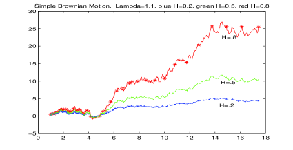
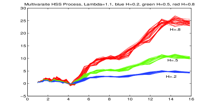
Figure 1: Simple Brownian Motion and corresponding Multivariate H-ss Process where Scales and Hurst index are indicated .               above the figures

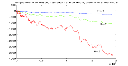
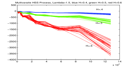
Figure 2: Simple Brownian Motion and corresponding Multivariate H-ss Process where Scales and Hurst index are indicated .                above the figures

All the multi-dimensional self-similar processes have been plotted at points $\lambda^{n}$ where $n=0,1,2,\cdots,M$. One can easily verify that how SBM’s are going to enlarge at the beginning of each scale interval $[\lambda^{n-1},\lambda^{n})$, which is the main property of DSI processes, while for the corresponding multi-dimensional self-similar process, which have been constructed by one observation in each scale interval, these jumps are equally like for all observations. Figure 1, consists of two figures SBM on the left and corresponding multi-dimensional self-similar on the right. The figure on the left consists of three different curves of SBM, all with scale $\lambda=1.1$, but with different Hurst index. It is worthy to note that we have simulated just one discrete time Brownian motion $B(\lambda^{n}{\bf s}_{i})$ of Example 4.1, for these three curves. The curve in the middle has Hurst index $H=0.5$, so it is a discrete time Brownian motion which is a self-similar process and other two curves are to compare with this. The upper curve has Hurst index $H=0.8$, so it is a scale invariant process and at the beginning of each scale interval $[\lambda^{n-1},\lambda^{n})$ enlargement in compare with Brownian motion occurs, which has been caused by the growth of coefficients to $\lambda^{n(0.8-1/2)}$ at the beginning of $n$-th scale interval. Also the lower curve has scale $H=0.2$, so in compare with Brownian motion, the coefficient at the beginning of $n$-th scale interval decreases to $\lambda^{n(0.2-1/2)}$. So it comes to have less variation than Brownian Motion at the beginning of each scale interval. Figure 2 is also included of two figures, where the left one again consist of three curves of SBM all with scale $\lambda=1.5$, but with Hurst indices $H=0.4,0.5$ and $0.6$. Again we have generated one $B(t)$ for all these three curves. The curve in the middle has Hurst index $H=0.5$, so is a Brownian motion. The upper curve is SBM with $H=0.6$, where enlargement in compare to Brownian motion occurs at the beginning of scale intervals by $\lambda^{n(0.6-1/2)}$ and to the same direction of the Brownian motion, the middle curve. The curve with $H=0.4$, lower curve , has less variation in compare with Brownian motion. So the size of lines at the beginning of all scale intervals decreases,by the rate $\lambda^{n(0.4-1/2)}$ with respect to the Brownian motion, for the $n$-th scale interval. For the corresponding multi-dimensional self-similar processes where the $i$-th curve, for $i=0,\ldots,q-1$ has been evaluated at sample points $\big{\{}\lambda^{n}{\bf s}_{i},n\in{\mathbb{Z}}\big{\}}$ of corresponding SBM, and has been plotted at points $\lambda^{n}$, and all are self-similar with the same Hurst index. Finally the growth of Hurst index causes the growth of all lines in the corresponding multi-dimensional self-similar process as well.

One can compare these multi-dimensional self-similar processes with the corresponding SBM which shows that as these are close together at any point $\lambda^{n}$, the changes inside the corresponding scale interval are less. It is also interesting that as at the end points of the multivariate self-similar process for $H=0.8$, have more variation , so the variation inside last scale intervals of SBM with $H=0.8$ is more. Finally as the path of all multi-dimensional self-similar for $H=0.8$ and $\lambda=1.5$ for last observations are decreasing, and for $H=0.8$ and $\lambda=1.1$ are increasing, so the path of corresponding SBM at the beginning of last scale intervals are respectively decreasing and increasing.

References

• [1] P. Borgnat, P.O. Amblard, P. Flandrin, 2005, ”Scale invariances and Lamperti transformations for stochastic processes”, Journal of Physics A: Mathematical and General, Vol.38, pp.2081 2101.
• [2] M.E. Caballero, L. Chaumont, 2006, ”Weak convergence of positive self-similar Markov processes and overshoots of Levy processes”, The annals of probability, Vol.34, No.3, pp.1012-1034.
• [3] J.L. Doob, ”Stochastic Processes”, Wiley, New York 1953.
• [4] P. Flandrin, P. Borgnat, P.O. Amblard, 2002, ”From stationarity to selfsimilarity, and back : Variations on the Lamperti transformation”, appear in Processes with Long-Range Correlations, pp.88-117.
• [5] E.G. Gladyshev, 1961, ”Periodically correlated random sequences”, Soviet Math. Dokl., No.2, pp.385-388.
• [6] N. Modarresi, S. Rezakhah, 2010, ”Spectral analysis of Multi-dimensional self-similar Markov processes”, Journal of Physics A: Mathematical and Theoretical, Vol.43, No.12, 125004 (14pp).
• [7] Y.A. Rozanov, 1967, ”Stationary Random Processes”, Holden-Day, San Francisco.
• [8] C.J. Nuzman, H.V. Poor, ”Linear estimation of self-similar processes via Lamperti s transformation”, Journal of Applied Probability, No.37(2), 2000.