Using Radio Halos and Minihalos to Measure the Distributions
of Magnetic Fields and Cosmic-Rays in Galaxy Clusters

Abstract

Some galaxy clusters show diffuse radio emission in the form of giant halos (GHs) on Mpc scales or minihalos (MHs) on smaller scales. Comparing Very Large Array and XMM-Newton radial profiles of several such clusters, we find a universal linear correlation between radio and X-ray surface brightness, valid in both types of halos. It implies a halo central emissivity $\nu j_{\nu}=10^{-31.4\pm 0.2}(n/10^{-2}\mbox{ cm}^{-3})^{2}(T/T_{0})^{0.2\pm 0.5}\mbox{ erg}\mbox{ s}^{-1}\mbox{ cm}^{-3}$, where $T$ and $T_{0}$ are the local and central temperatures, and $n$ is the electron number density. We argue that the tight correlation and the scaling of $j_{\nu}$, combined with morphological and spectral evidence, indicate that both GHs and MHs arise from secondary electrons and positrons, produced in cosmic-ray ion (CRI) collisions with a strongly magnetized, $B\gtrsim 3\mbox{ $\mu$G}$ intracluster gas. When the magnetic energy density drops below that of the microwave background, the radio emission weakens considerably, producing halos with a clumpy morphology (e.g., RXC J2003.5 -2323 and A2255) or a distinct radial break. We thus measure a magnetic field $B=3\mbox{ $\mu$G}$ at a radius $r\simeq 110\mbox{ kpc}$ in A2029 and $r\simeq 50\mbox{ kpc}$ in Perseus. The spectrum of secondaries, produced from hadronic collisions of $\sim 20\mbox{ GeV}$ CRIs, reflects the energy dependence of the collision cross section. We use the observed spectra of halos, in particular where they steepen with increasing radius or frequency, to (i) measure $B\simeq 10(\nu/700\mbox{ MHz})\mbox{ $\mu$G}$, with $\nu$ the spectral break frequency; (ii) identify a correlation between the average spectrum and the central magnetic field; and (iii) infer a CRI spectral index $s\lesssim-2.7$ and energy fraction $\xi_{p}\sim 10^{-3.6\pm 0.2}$ at particle energies above 10 GeV. Our results favor a model where CRIs diffuse away from their sources (which are probably supernovae, according to a preliminary correlation with star formation), whereas the magnetic fields are generated by mergers in GHs and by core sloshing in MHs.

1. Introduction

Giant halos (GHs) appear as diffuse radio emission on $\sim\mbox{Mpc}$ scales in merging galaxy clusters (for a review, see Feretti & Giovannini, 2008). GHs were identified in about a quarter of all clusters with X-ray luminosities $L_{X}>5\times 10^{44}\mbox{ erg}\mbox{ s}^{-1}$ at redshifts $0.2<z<0.4$ (Brunetti et al., 2007). $L_{X}$ and the specific radio power $P_{\nu}$ of GH clusters are tightly correlated. The GH distribution in clusters is bimodal, with most clusters showing no associated GH at a sensitivity threshold $\sim 10$ times better than the signal expected from the $L_{X}$–$P_{\nu}$ correlation (Brunetti et al., 2007).

GHs arise from synchrotron radiation, emitted by cosmic-ray electrons and positrons (CREs) injected locally and continuously into the magnetized plasma. Such CREs can lose a considerable fraction of their energy by inverse-Compton scattering off the cosmic microwave background (CMB). Recently, Kushnir et al. (2009, henceforth K09) made the important observation that the GH properties mentioned above are reproduced if the CREs are produced in $p$-$p$ cosmic ray proton (CRP) collisions, and the magnetic field $B$ is sufficiently strong to saturate $P_{\nu}(B)$ by rendering Compton losses negligible.

To qualitatively see this, assume that the CRP number density $n_{p}$ is (narrowly distributed about) a universal fraction of the local (non cosmic-ray) electron number density $n$, and that the magnetic energy density greatly exceeds the energy density $u_{cmb}$ of the CMB, $B\gg B_{cmb}\equiv(8\pi u_{cmb})^{1/2}$. Here, the ratio between the emissivities of radio synchrotron $j_{\nu}\propto n_{p}nB^{2}/(B^{2}+B_{cmb}^{2})\propto n^{2}$ (from secondary, density $n_{e}\propto n_{p}n$ CREs) and X-ray bremsstrahlung $j_{X}\propto n^{2}$ (from the thermal plasma), does not depend on $n$ or on $B$. Thus, strongly magnetized clusters with $B\gtrsim B_{cmb}$ would show a strong radio-X-ray correlation, whereas clusters with $B\lesssim B_{cmb}/3$ would be too radio faint to show a GH. Other models, notably turbulent reacceleration of electrons (for a review see Petrosian & Bykov, 2008), do not naturally produce the correlation and bimodality that are observed.

Radio minihalos (MHs) are found in cool core clusters (CCs). They extend roughly over the cooling region (Gitti et al., 2002), encompassing up to a few percent of the typical GH volume. Detecting MHs is more challenging than GHs, due to their smaller size and proximity to an active galactic nucleus (AGN), so only few MHs have been well studied and less is known about their correlation with X-rays. A morphological association between MH edges and cold fronts (CFs; Mazzotta & Giacintucci, 2008) suggests a link between MHs and sloshing activity in the core. Such CFs are observed in about half the CCs, and are probably present in many more (Markevitch & Vikhlinin, 2007). They are thought to be tangential discontinuities that isolate regions magnetized by bulk shear flow at smaller radii (Keshet et al., 2010) (regions we refer to as below, or inside the CF).

There are many similarities between GHs and MHs. Both types of halos are usually characterized by a regular morphology, low surface brightness, little or no polarization, and spectral indices $\alpha_{\nu}\equiv d\log(P_{\nu})/d\log\nu\simeq-(1.0-1.5)$, with $\nu$ the frequency. However, there are telling exceptions to these characteristics. A few GHs have a clumpy or filamentary morphology, such as in RXC J2003.5 -2323 (Giacintucci et al., 2009), A2255, and A2319 (Murgia et al., 2009, henceforth M09). Strong polarization was so far detected in one GH (at a $20\%$–$40\%$ level, in A2255; see Govoni et al. (2005); weaker polarization, $2-7\%$ on average, was found in MACS J0717.5 +3745; see Bonafede et al. (2009)), and in one MH (at a $10\%-20\%$ level, in A2390; Bacchi et al., 2003). Spectral steepening with increasing $r$, increasing $\nu$, or decreasing $T$, has been reported in several radio halos (Feretti & Giovannini, 2008; Ferrari et al., 2008; Giovannini et al., 2009, and references therein); typically, $\alpha$ steepens from $-1.0$ to $-(1.3$–$1.5)$ in uncontaminated regions (see §5.2). A handful of GHs show a steep, $\alpha<-1.5$ spectrum, such as in A521 ($\alpha=-1.86\pm 0.08$; Dallacasa et al., 2009) and in A697 ($\alpha=-(1.7$–$1.8)$; Macario et al., 2010).

We analyze a sample of GHs and MHs using radio and X-ray data from the literature. We find a universal correlation between the radio and X-ray surface brightness, which holds for both types of halos. This correlation, combined for example with the observed dependence of the radio bright volume fraction upon cluster parameters (Cassano et al., 2007), gives rise to the luminosity correlation known in GHs, and a similar correlation that we derive for MHs. We determine the radio emissivity $j_{\nu}$ and its scaling with electron density and temperature $T$, using the surface brightness correlation and a model (XSPEC/MEKAL) for the X-ray emission. Combined with other properties of GHs and MHs, this singles out secondary CRE models with strong magnetic fields for both types of halos. This generalizes the GH model of K09, and, considering the different environments of GHs and MHs, substantially strengthens it. We propose that the cosmic-ray ions (CRIs) are produced in supernovae, based on the halo spectra, the $j_{\nu}$ scaling, and a preliminary correlation between star formation and the radio to X-ray brightness ratio ${\eta}$. We show how the spectral and morphological properties of halos can be used to disentangle the distributions of CREs and magnetic fields. In particular, the magnetic field is gauged both by a radial break in ${\eta}$ reflecting the onset of Compton losses, and by a spectral break in radio emission induced by diffractive p–p scattering.

The paper is arranged as follows. In §2 we show that GHs and MHs follow the same correlation between specific radio power and coincident X-ray luminosity, suggesting that the different types of halos arise from similar processes. A tight, universal correlation between the surface brightness in radio and in X-rays is presented in §3. It is used to derive the scaling of radio emissivity with the local electron number density $n$ and temperature $T$, and to explain previous results for the average halo emissivity and the luminosity correlation. We then show in §4 that the inferred scaling favors a model in which the radio emission in both GHs and MHs originates from secondary CREs produced by collisions of CRIs with the intracluster gas, synchrotron radiating most of their energy in strong magnetic fields. We study the morphological and spectral properties of the halos in §5, presenting new methods for measuring the distributions of CRIs and magnetic fields. Finally, we discuss the origin of the CRIs and magnetic fields in §6, and summarize our results. We assume a Hubble constant $H=70\mbox{ km}\mbox{ s}^{-1}\mbox{ Mpc}^{-1}$. Error bars are $1\sigma$ confidence intervals.

2. GHs and MHs: similar correlation between radio and coincident X-ray emission

The 19 X-ray bright GH clusters in the Brunetti et al. (2007) sample follow the correlation

$$(\nu P_{\nu,1.4})_{45}\simeq 10^{-4.2\pm 0.3}L_{X[0.1,2.4],45}^{1.7}\mbox{ ,}$$ (1)

where the subscript $45$ denotes units of $10^{45}\mbox{ erg}\mbox{ s}^{-1}$. Here, $X[\epsilon_{1},\epsilon_{2}]$ designates integration over photon energies between $\epsilon_{1}$ and $\epsilon_{2}$ measured in keV (we use $X[0.1,2.4]$ unless otherwise stated), and subscript $1.4$ means that the radio signal is evaluated at a frequency $\nu=1.4\mbox{ GHz}$. The normalization uncertainty in Eq. (1) is dominated by an intrinsic scatter among halos, needed to obtain an acceptable fit (chosen as $\chi^{2}/N=1$ with $N$ being the number of degrees of freedom). Accounting for dispersion in $P_{\nu}$ leads to the correlation in the form of Eq. (1), in agreement with K09, somewhat flatter than in Cassano et al. (2006).

A sample of $6$ well-studied MHs had been reported (Cassano et al., 2008) as being “barely” consistent with the GH correlation of Cassano et al. (2006). However, we find that this sample agrees well with Eq. (1) with $\chi^{2}/N=1.4$. Nevertheless, within a partly overlapping sample of 6 MHs studied recently (Govoni et al., 2009, M09), the MHs appear significantly underluminous with respect to the prediction of Eq. (1) after a careful removal (M09) of the contamination from AGNs.

These results do not imply that MHs are intrinsically fainter than GHs. Rather, MHs have comparable radio power, if one corrects for their smaller size. A natural generalization of Eq. (1) applicable for both GHs and MHs would replace $L_{X}$ with the luminosity $\bar{L}_{X}$ of the radio bright region. Following M09, we define the radio bright region based on the surface brightness condition $I_{\nu}(r)/I_{\nu}(r=0)>e^{-3}\simeq 5\%$, with $r$ being the radial distance from the cluster center; equivalently, the radius of this region is $R_{\nu}=3r_{e}$, with $r_{e}$ being the e-fold radius.

A quick way to estimate $\bar{L}_{X}$ is to correct $L_{X}$ using a model for the X-ray brightness profile of the cluster. Using an isothermal $\beta$-model (Cavaliere & Fusco-Femiano, 1976), in which $n(r)=n_{0}(1+r^{2}/r_{c}^{2})^{-3\beta/2}$ for model parameters $\beta$, $r_{c}$ and $n_{0}$, we find that

$$\bar{L}_{X}=L_{X}\frac{\left(1+R_{\nu}^{2}/r_{c}^{2}\right)^{\frac{3}{2}-3\beta}-1}{\left(1+R_{X}^{2}/r_{c}^{2}\right)^{\frac{3}{2}-3\beta}-1}\mbox{ .}$$ (2)

We use individual cluster $\beta$-model parameters from the literature; see Table 1 for details. The radius $R_{X}$ of the X-ray region considered must be finite in order to ensure convergence. Its choice is somewhat arbitrary; we use $R_{X}=12r_{c}$ so $R_{\nu}<R_{X}$ for all halos in the M09 sample.

l (1) (2) (3) (4) (5) (6) (7) (8) (9) (10) (11) (12) (13) Cluster Type $z$ $L_{X[0.1-2.4]}$ $T$ $r_{e}$ $\langle j\rangle$ $\beta$ $r_{c}$ $\bar{L}_{X[0.1-2.4]}$ $B_{0,min}$ $\langle\alpha\rangle$ $Z(0.1r_{500})$ A401 GH $0.074$ $6.3_{-0.1}^{+0.1}$ (R02) $7.8_{-0.2}^{+0.2}$ (A09a) $109_{-15}^{+21}$ $4.1_{-1.0}^{+1.3}$ $0.61_{-0.01}^{+0.01}$ (C07) $175_{-7.1}^{+7.9}$ $3.1_{-0.1}^{+0.1}$ $7.5$ $\alpha_{0.6}^{1.4}=-1.4$ (R81) — A545 GH $0.154$ $5.7_{-0.5}^{+0.5}$ (C06) $5.5_{-2.1}^{+6.2}$ (D93) $150_{-11}^{+11}$ $12.0_{-1.9}^{+2.2}$ — — — — $\alpha_{1.4}<-1.4$ (G03) — A665 GH $0.182$ $9.8_{-1.0}^{+1.0}$ (C06) $7.9_{-0.2}^{+0.2}$ (A09a) $236_{-15}^{+18}$ $7.0_{-1.0}^{+1.0}$ $0.54_{-0.01}^{+0.01}$ (B06) $139_{-4.2}^{+4.2}$ $7.1_{-1.0}^{+1.0}$ $17.1$ $\alpha_{0.3}^{1.4}=-1.04_{-0.02}^{0.02}$ (F04b) $0.30\pm 0.06$ A773 GH $0.217$ $6.1_{-0.5}^{+0.5}$ (B00) $7.4_{-0.3}^{+0.3}$ (A09a) $111_{-10}^{+10}$ $11.0_{-2.0}^{+2.4}$ $0.61_{-0.01}^{+0.01}$ (B06) $131_{-4.2}^{+4.2}$ $3.7_{-0.5}^{+0.5}$ $12.1$ $\alpha_{0.3}^{1.4}=-1.02_{-0.26}^{+0.26}$ (K01) $0.41\pm 0.16$ A2163 GH $0.203$ $17.1_{-0.3}^{+0.3}$ (R02) $14.7_{-0.3}^{+0.3}$ (V09) $394_{-7}^{+7}$ $9.2_{-0.4}^{+0.4}$ $0.80_{-0.03}^{+0.03}$ (C07) $371_{-20.7}^{+21.4}$ $15.2_{-0.3}^{+0.3}$ $19.9$ $\alpha_{0.07}^{1.4}=-1.02$ (V09) $0.25\pm 0.07$ A2218 GH $0.176$ $4.6_{-0.2}^{+0.2}$ (E98) $7.2_{-0.2}^{+0.2}$ (A09a) $76_{-18}^{+26}$ $20.0_{-9.0}^{+14.0}$ $0.77_{-0.01}^{+0.01}$ (B06) $190_{-4.3}^{+4.6}$ $2.4_{-0.2}^{+0.2}$ $7.5$ $\alpha_{0.3}^{1.4}=-1.46_{-1.0}^{1.0}$ (K01) $0.37\pm 0.15$ A2219 GH $0.226$ $12.7_{-1.0}^{+1.0}$ (C06) $9.5_{-0.4}^{+0.6}$ (C06) $359_{-14}^{+18}$ $5.4_{-0.6}^{+0.6}$ $0.66_{-0.01}^{+0.07}$ (F04) $208_{-23.8}^{+99.1}$ $11.2_{-1.0}^{+1.0}$ $25.3$ $\alpha_{0.3}^{1.4}=-0.9_{-0.1}^{+0.1}$ (O07) — A2254 GH $0.178$ $4.3_{-0.4}^{+0.4}$ (B00) $7.5_{-1.5}^{+0.5}$ (C06) $238_{-39}^{+57}$ $9.7_{-2.8}^{+3.4}$ — — — — $\alpha_{1.4}^{1.7}\sim-1.2$ (G01) — A2255 GH $0.081$ $2.6_{-0.1}^{+0.1}$ (C06) $6.9_{-0.1}^{+0.1}$ (A09a) $203_{-6}^{+6}$ $3.4_{-0.2}^{+0.2}$ $0.80_{-0.03}^{+0.03}$ (C07) $424_{-22.9}^{+25.0}$ $1.7_{-0.1}^{+0.1}$ $7.4$ $\alpha_{0.3}^{1.4}=-2.06_{-0.57}^{+0.57}$ (K01) — A2319 GH $0.056$ $8.2_{-0.1}^{+0.1}$ (C07) $8.8_{-0.2}^{+0.3}$ (C06) $198_{-6}^{+7}$ $5.4_{-0.4}^{+0.4}$ $0.59_{-0.01}^{+0.01}$ (C07) $203_{-9.3}^{+10.0}$ $5.1_{-0.1}^{+0.1}$ $3.8$ $\alpha_{0.3}^{1.4}=-1.28_{-0.35}^{+0.35}$ (K01) $0.31\pm 0.04$ A2744 GH $0.308$ $13.1_{-2.4}^{+2.4}$ (C06) $8.6_{-0.3}^{+0.4}$ (C06) $275_{-9}^{+9}$ $25.0_{-1.6}^{+1.7}$ $0.57_{-0.06}^{+0.12}$ (F04) $251_{-2.4}^{+120}$ $8.1_{-2.4}^{+2.4}$ $16.0$ $\alpha_{0.07}^{1.4}=-1.1$ (V09) — RXJ1314 GH $0.244$ $7.3_{-0.7}^{+0.7}$ (M01) $8.7_{-0.4}^{+0.4}$ (M01) $160_{-38}^{+61}$ $12.0_{-5.0}^{+8.0}$ $0.77_{-0.23}^{+0.23}$ (V02) $286_{-100}^{+100}$ $4.9_{-0.7}^{+0.7}$ $10.9$ $\alpha_{0.07}^{1.4}=-1.4$ (V09) — A1835 MH $0.253$ $16.3_{-1.2}^{+1.2}$ (B00) $7.1_{-0.1}^{+0.1}$ (A09a) $102_{-31}^{+70}$ $33.0_{-13.0}^{+22.0}$ $0.53_{0.00}^{+0.00}$ (S08) $29.0_{-0.3}^{+0.3}$ $15.6_{-1.2}^{+1.2}$ $33.1$ — $0.28\pm 0.05$ A2029 MH $0.076$ $8.5_{-0.1}^{+0.1}$ (C07) $6.9_{-0.1}^{+0.1}$ (A09a) $53_{-6}^{+6}$ $54.0_{-13.0}^{+19.0}$ $0.58_{0.00}^{+0.00}$ (C07) $59.3_{-1.4}^{+1.4}$ $4.9_{-0.1}^{+0.1}$ $8.3$ $\alpha_{0.2}\simeq-1.35$ (S83) $0.38\pm 0.06$ A2390 MH $0.228$ $15.8_{-0.2}^{+0.2}$ (A03) $9.3_{-0.1}^{+0.1}$ (B07) $36_{-4}^{+4}$ $3100_{-800}^{+1000}$ $0.47_{0.00}^{+0.00}$ (S08) $46.0_{-1.0}^{+1.0}$ $5.3_{-0.2}^{+0.2}$ $9.5$ $\alpha_{0.07}^{0.4}\simeq-1.10$ (A06) — Ophiuchus MH $0.028$ $6.1_{-0.2}^{+0.2}$ (C07) $10.2_{-0.4}^{+0.3}$ (C07) $105_{-11}^{+13}$ $4.7_{-0.8}^{+0.9}$ $0.75_{-0.03}^{+0.04}$ (C07) $199_{-15.0}^{+16.4}$ $3.8_{-0.2}^{+0.2}$ $6.9$ — — Perseus MH $0.018$ $8.2_{-0.1}^{+0.1}$ (C07) $6.4_{-0.1}^{+0.1}$ (F04) $23_{-1}^{+1}$ $3600_{-500}^{+500}$ $0.54_{0.00}^{+0.01}$ (C07) $45.0_{-0.7}^{+1.4}$ $2.5_{-0.1}^{+0.1}$ $4.8$ $\alpha_{0.3}^{1.5}\sim-1.2$ (G04) $0.42\pm 0.01$ RXJ1347 MH $0.451$ $27.5_{-1.1}^{+1.1}$ (F04) $10.7_{-0.1}^{+0.1}$ (A09b) $52_{-11}^{+17}$ $1800_{-500}^{+700}$ $0.54_{0.00}^{+0.00}$ (B06) $23.3_{-0.5}^{+0.5}$ $22.6_{-1.1}^{+1.1}$ $32.4$ — $0.39\pm 0.04$
Columns: (1) cluster name (1RXS J131423 .6-251521 abbreviated RXJ1314; RXJ1347.5-1145 abbrev. RXJ1347); (2) halo type (GH or MH); (3) redshift $z$; (4) X-ray luminosity between $0.1$ and $2.4\mbox{ keV}$, in units of $10^{44}\mbox{ erg}\mbox{ s}^{-1}$; (5) temperature in keV; (6) e-fold radius of radio brightness in kpc (M09); (7) average $1.4\mbox{ GHz}$ specific emissivity in units of $10^{-43}\mbox{ erg}\mbox{ s}^{-1}\mbox{ cm}^{-3}\mbox{ Hz}^{-1}$ (M09); (8-9) exponent $\beta$ and core radius $r_{c}$ in kpc for an isothermal $\beta$-model of the cluster; (10) X-ray luminosity of the radio bright region (see §2) between $0.1$ and $2.4\mbox{ keV}$, in units of $10^{44}\mbox{ erg}\mbox{ s}^{-1}$; (11) minimal central magnetic field $B_{0,min}$ in units of $\mu$G, assuming the $\beta$-model and that $B(r=\min\{r_{b},3r_{e}\})=B_{cmb}$ (corresponding to $f_{ic}=0.5$ in Eq. 12), where the radial break radius $r_{b}=55\mbox{ kpc}$ in Perseus, $135\mbox{ kpc}$ in A2029, $60\mbox{ kpc}$ in A2319, and $r_{b}>3r_{e}$ in the other halos; (12) average spectral index $\alpha_{\nu_{1}}^{\nu_{2}}$ between frequencies (in GHz) $\nu_{1}$ and $\nu_{2}$, or $\alpha_{\nu}$ around frequency $\nu$; (13) Metallicity measured at $r=0.1r_{500}$ in solar units (Snowden et al., 2008).

References: References are given in parentheses. For conflicting references, we adopt the tighter estimate if applicable, and otherwise use the most recent result. A03: Allen et al. (2003); A06: Augusto et al. (2006); A09a: Andersson et al. (2009); A09b: Anderson et al. (2009); B00: Böhringer et al. (2000); B03: Bacchi et al. (2003); B06: Bonamente et al. (2006); B07: Baldi et al. (2007); C06: Cassano et al. (2006); C07: Chen et al. (2007); D93: David et al. (1993); F04: Fukazawa et al. (2004); F04b: Feretti et al. (2004a) F07: Feretti et al. (1997); G01: Govoni et al. (2001b); G03: Giovannini et al. (2003); G04: Gitti et al. (2004); H80: Harris et al. (1980); K01: Kempner & Sarazin (2001); M00: Matsumoto et al. (2000); M01: Matsumoto et al. (2001); M07: Morandi et al. (2007); R81: Roland et al. (1981) R02: Reiprich & Böhringer (2002); S83: Slee & Siegman (1983); S08: Santos et al. (2008); S09: Sanderson et al. (2009); V02: Valtchanov et al. (2002); V09: van Weeren et al. (2009); WB03: Worrall & Birkinshaw (2003); W00: White (2000).

Table 1 Parameters of Halo Clusters in the Sample

Figure 1 shows various GHs and MHs in the resulting $\bar{L}_{X}-\nu P_{\nu}$ plane. Replacing $L_{X}$ by $\bar{L}_{X}$ results in slightly better agreement of the M09 GHs with Eq. (1), yielding $\chi^{2}/N=1.3$ instead of 1.6 (before propagating $\beta$ model uncertainties). However, the MH agreement becomes much better, $\chi^{2}/N=2.4$ instead of 3.7. Note that the fit is not expected to be as good for MHs as it is for GHs, because a $\beta$-model is less appropriate for a CC. These results suggest that the relation between radio and X-ray emission is similar in GHs and in MHs. For more accurate, model-independent results, we next examine a more local measure of the emission, and consider the radio and X-ray morphologies.

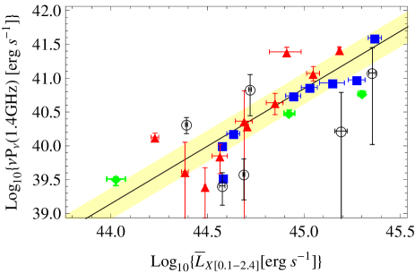
Figure 1.— Radio power $\nu P_{\nu}$ at $1.4\mbox{ GHz}$ of GHs (red triangles) and MHs (black circles) from M09, plotted against the 0.1-2.4 keV X-ray luminosity $\bar{L}_{X}$ of the radio bright region (see §2 and table 1 for details). The total X-ray luminosity $L_{X}$ is used in cases where $\bar{L}_{X}$ could not be determined, for GHs (blue squares, from Cassano et al., 2006) and MHs (green diamonds, from Cassano et al., 2008). The solid line and shaded region show the best fit and $1\sigma$ interval of the GH correlation in Eq. (1).

3. Correlation between Radio and X-ray surface brightness: universal emissivity

A more useful manifestation of the radio-X-ray correlation is the morphological similarity between radio and X-ray emission. A linear correlation between the radio surface brightness $I_{\nu}$ and the X-ray brightness $F_{X}$ was found by Govoni et al. (2001a) in two GH clusters (A2744 and A2255, inspected individually), while a sublinear power law was found in two other GHs (A2319 and Coma).

We investigate the connection between the radio and the X-ray surface brightness in GH and MH clusters by examining the radial brightness profiles published in the literature. We consider not only the radio to X-ray relation within each cluster, but also compare the ratio between $\nu I_{\nu}$ and $F_{x}$ in different clusters. Thus, Figure 2 shows the radial profile of the dimensionless ratio

$${\eta}(r)\equiv\frac{\nu I_{\nu}(1.4\mbox{ GHz})}{F_{X[0.1-2.4]}}$$ (3)

between radio and X-ray surface brightness, for all six GHs and four MHs with published radial profiles from both Very Large Array (VLA; M09) and XMM-Newton (Snowden et al., 2008) observations. Distances are normalized to $r_{500}$, the radius enclosing $500$ times the critical density of the Universe (calculated using the best fit of Zhang et al., 2008).

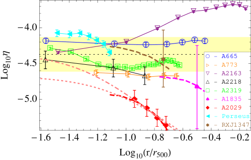
Figure 2.— Radial profiles of the radio-to-X-ray ratio ${\eta}$ (defined in Eq. (3)) in the GHs (open symbols) and MHs (filled symbols) with overlapping profiles from VLA (M09) and from XMM-Newton (Snowden et al., 2008, k-corrected). The MH data is shown only in regions where the AGN contamination is $<10\%$; this is supplemented by the exponential model fits (dashed curves) given by M09, plotted in the range where radio detection is $>3\sigma$ and the MH contribution is $>30\%$. Error bars are the $1\sigma$ confidence intervals of the radio normalization $I_{0}$ (M09), and the solid lines serve to guide the eye. The $1\sigma$ best fit of Eq. (4) is shown as a thin dashed line in a shaded region. Model fits for A2029 (dotted and dot-dashed curves; see §5.1) are also shown.

All halo clusters except the MH in A2029 converge on a similar value of ${\eta}$ at small radii. The innermost GH data is best fit by

$${\eta}_{0}\equiv{\eta}(r=0)=10^{-4.4\pm 0.2}\mbox{ ,}$$ (4)

where the uncertainty is again larger than the measurement errors and mostly attributed to intrinsic scatter between halos. The inner MH data also lie within the $1\sigma$ scatter, except A2029 which is significantly fainter in radio (but is observed only where ${\eta}(r)$ rapidly declines). Therefore, Eq. (4) appears to hold at small radii for both GHs and MHs. A possible explanation for the relatively high radio brightness of Perseus and A665, and the low brightness of A2029, is discussed in §6.2. As in §2, we used only GHs, which are better understood than MHs, to derive the correlation Eq. (4). If, instead, we use the innermost data of both GHs and MHs, we obtain a broader best fit, $\eta_{0}\simeq 10^{-4.4\pm 0.4}$, due to the bright MH in Perseus and the faint MH in A2029.

Although there is some scatter among different clusters, Fig. 2 shows that ${\eta}$ is fairly uniform within each GH. An exception is A2163, in which ${\eta}(r)$ monotonically increases out to $r\simeq 0.6r_{500}\simeq 1200\mbox{ kpc}$. However, this is the only cluster shown in Fig. 2 that harbors a radio relic (Feretti et al., 2001), which dominates the emission near the ${\eta}$ maximum (M09, figure 3). This suggests that the peculiar ${\eta}$ profile in A2163 is associated with the radio relic. A peculiar ${\eta}(r)$ pattern is seen in A2319, with a minimum at $r\simeq 0.1r_{500}\simeq 150\mbox{ kpc}$. Interestingly, this cluster shows both GH and MH characteristics, harboring both a CF at $r\simeq 100$–$200\mbox{ kpc}$ and a subcluster at $r\simeq 500\mbox{ kpc}$ (Govoni et al., 2004). In §5.1 we argue that the clumpy radio morphology of this cluster suggests weak magnetization, enhanced at both small and large radii in an intermediate phase between a GH and a MH. The declining ${\eta}(r)$ profiles of the MHs are discussed in §5.1.

In order to derive the radio emissivity from the brightness correlation Eq. (4), we must model the X-ray emission. The X-ray emissivity calculated using the MEKAL model (Mewe et al., 1985, 1986; Kaastra, 1992; Liedahl et al., 1995) in XSPEC v.12.5 (Arnaud, 1996) is nearly independent of temperature and metallicity. It is given by

$$j_{X[0.1-2.4]}\simeq 8.6\times 10^{-28}\frac{n_{-2}^{2}Z_{0.3}^{0.04}}{T_{10}^{0.1}}\mbox{ erg}\mbox{ s}^{-1}\mbox{ cm}^{-3}\mbox{ ,}$$ (5)

where $n_{-2}$ is the electron number density $n$ in units of $10^{-2}\mbox{ cm}^{-3}$, $T_{10}\equiv(k_{B}T/10\mbox{ keV})$ with $k_{B}$ being Boltzmann’s constant, and $Z_{0.3}$ is the metallicity $Z$ in units of $0.3Z_{\odot}$.

Fairly uniform values of ${\eta}$ are found within each cluster (excluding the outer regions of A2163), and similar values are found among different halos, in regions spanning two orders of magnitude in density. This implies that the radio emissivity $j_{\nu}$, like $j_{X}$, scales as the gas density squared. Indeed, M09 recently found (in their section 5.1) that assuming $j_{\nu}\propto n^{2}$ reproduces the radial profiles of some GHs and MHs. We conclude that the linear surface brightness relation Eq. (4) reflects a similar, local relation between the radio and X-ray emissivities,

$$\nu j_{\nu}\simeq\eta_{0}j_{X}\mbox{ .}$$ (6)

We examine the temperature dependence of the radio emissivity within a given cluster by fitting ${\eta}$ in uncontaminated GHs as a power law, such that $j_{\nu}\propto n^{2}(T/T_{0})^{{\kappa}}$, with $T_{0}$ being the central temperature and ${{\kappa}}$ being a free parameter. This yields ${{\kappa}}=0.2\pm 0.5$, consistent with weak or no temperature dependence within the cluster. Combining this with the above results Eqs. (4)-(6), we conclude that the synchrotron emissivity in halos is well fit by

$$\nu j_{\nu}\simeq 10^{-31.4\pm 0.2}n_{-2}^{2}(T/T_{0})^{0.2\pm 0.5}\mbox{ erg}\mbox{ s}^{-1}\mbox{ cm}^{-3}\mbox{ ,}$$ (7)

at least near the centers of the halos.

The scatter in Eqs. (4) and (7) indicates that the radio emissivity is not a function of the local density and temperature alone. The dispersion in $j_{\nu}$ probably reflects dependence upon additional cluster properties, such as the cluster’s mass and star formation history. It has standard deviation $\sigma(\log j_{\nu})\simeq\log(1.6)$ among the GHs in our sample, or $\sigma(\log j_{\nu})\simeq\log(2.5)$ if we include the MHs. This relatively small dispersion explains the similar volume-averaged emissivity ${\langle{j_{\nu}}\rangle}$ of different GHs, and the high level of variation in ${\langle{j_{\nu}}\rangle}$ among MHs, where ${\langle{j_{\nu}}\rangle}$ is sometimes two orders of magnitude larger than in GHs, as reported by Cassano et al. (2008) and M09; see Table 1. Indeed, the GHs in their sample have comparable sizes and central densities $n_{0}\simeq 10^{-2}\mbox{ cm}^{-3}$, whereas the MHs have variable scale and $n_{0}>10^{-1}\mbox{ cm}^{-3}$ in some cases.

We have derived linear relations between the radio and X-ray emissivity (Eq. 6) and surface brightness (Eqs. 3 and 4) of halos, but a superlinear, $P_{\nu}\propto L_{x}^{1.7}$ relation between the integrated luminosity in the two bands (Eq. 1). This indicates that, in addition to the $j_{\nu}\propto n^{2}(T/T_{0})^{\kappa}$ dependence, the total radio power of a halo must further increase, on average, with the mass and temperature of the cluster. Such a behavior could result in part from a (direct or indirect) mass or temperature dependence of $j_{\nu}$. However, the dispersion in $j_{\nu}$ is small, and we find no evidence for such a correlation. The effect is probably dominated by the different scalings of the radio and X-ray bright volumes with the cluster parameters, as we qualitatively show next.

The length scale $R_{\nu}$ of GHs was found to depend superlinearly on the virial radius $R_{vir}$, $R_{\nu}\sim R_{vir}^{\lambda_{R}}$, with $\lambda_{R}=2.6\pm 0.5$ (Cassano et al., 2007). In order to estimate the effect of this scaling on the $P_{\nu}$–$L_{X}$ correlation, we crudely approximate the luminosity within a sphere of radius $R$ as a power-law, $L(<R)\propto R^{\lambda_{L}}$. In a $\beta$-model, this is a poor approximation, with power-law indices $0.5<\lambda_{L}<2$ in the parameter range $0.5<\beta<0.7$, $1<r/r_{c}<4$, relevant to GHs. For simplicity, we assume that $L_{X}$ reflects the emission within a sphere of radius $\propto R_{vir}$. For constant ${\eta}$, we may then write

$$\frac{P_{\nu}}{L_{X}}\propto\left(\frac{R_{\nu}}{R_{vir}}\right)^{\lambda_{L}}\propto R_{vir}^{(\lambda_{R}-1)\lambda_{L}}\propto L_{X}^{0.3(\lambda_{R}-1)\lambda_{L}}\mbox{ ,}$$ (8)

where we used the observed scalings $R_{vir}\sim T^{0.6}$ (Zhang et al., 2008) and $L_{X}\sim T^{2}$ (Markevitch, 1998) in the last proportionality (recall that $X$ represents the energy range $0.1$–$2.4\mbox{ keV}$). Equation (8) yields $P_{\nu}\propto L_{X}^{(1.2-2.0)}$, where we accounted for the $\lambda_{L}$ range but have not propagated the scaling errors. While this demonstrates that the $R_{\nu}$–$R_{vir}$ scaling may suffice to reconcile the nonlinear luminosity relation Eq. (1) with the linear emissivity relation Eq. (6), much better modeling is required in order to identify all factors governing the luminosity correlation. For example, we neglected halo asymmetry and possible variations in ${\eta}$ at large radii (as in A2163).

4. Universal Radio Mechanism

In the preceding sections we examined the luminosity and surface brightness properties of GHs and MHs, in radio and in X-rays, and derived the radio emissivity, without making any assumptions regarding the particles and magnetic fields responsible for the radio emission. Here we explore the implications of the radio-X-ray correlation and the radio scalings derived above. In §4.1, we discuss various models for radio halos, and show that only models with strong magnetic fields and secondary CREs are consistent with the observations. In §4.2 we briefly discuss the effect of time dependent magnetic fields.

4.1. Secondary CREs, strong magnetic fields

The spectral slope near the center of most radio halos is $\alpha\simeq-1$ (see §5.2). A synchrotron spectrum of this type is emitted by rapidly cooling CREs, injected with approximately constant energy per decade in particle energy $E_{e}$. The synchrotron emissivity corresponding to a logarithmic CRE energy density injection rate $Q\equiv du_{e}/(dt\,d\ln E_{e})=\mbox{constant}$ is given by

$$\nu j_{\nu}\equiv\nu\frac{du_{\gamma}}{dt\,d\nu}=\frac{Q/2}{1+(B_{cmb}/B)^{2}}\mbox{ ,}$$ (9)

where the denominator accounts for Compton losses, $B_{cmb}\equiv(8\pi u_{cmb})^{1/2}\simeq 3.2(1+z)^{2}\mbox{ $\mu$G}$ is the amplitude of the magnetic field which has the same energy density as the CMB, and $u_{j}$ is the energy density of component $j$ ($\gamma$ for radio photons, $e$ for CREs, etc.). In the $B\gg B_{cmb}$ limit, the synchrotron emissivity Eq. (7) extracted from the observations yields a direct estimate of the CRE injection rate,

$$Q\simeq\frac{Q}{1+(B_{cmb}/B)^{2}}=10^{-31.1\pm 0.2}n_{-2}^{2}\mbox{ erg}\mbox{ s}^{-1}\mbox{ cm}^{-3}\mbox{ .}\,\,\,\,\,$$ (10)

As CREs do not have time to diffuse before they lose their energy, this result applies locally. It holds in both GHs and MHs.

The remarkably small scatter found in the radio-X-ray correlations among different GHs has been interpreted as implying a robust radio mechanism that keeps the synchrotron emissivity narrowly distributed around a universal function of the plasma density and perhaps also temperature. Equation (10) and the narrow scatter in its normalization suggest that the universal quantity in radio halos — both GHs and MHs — is $Q/n^{2}$.

Our results strongly emphasize the robustness of the radio emission mechanism. First, we find a tight radio-X-ray correlation not only in GHs but also in MHs. As the latter have physical properties that are considerably different from GHs (smaller size, higher ambient density, nearby AGN, CF association), the radio emission mechanism must be sufficiently robust to reproduce the same levels of $Q/n^{2}$ over a wide range of physical conditions. Second, we confirm that a tight radio-X-ray correlation exists not only in the total cluster luminosity but also in the local surface brightness, and that the ratio ${\eta}$ between radio and X-ray brightness is fairly uniform within each cluster. This is particularly striking in MHs, where the coincident density and temperature profiles are steep.

K09 have pointed out that in the strong magnetization regime, defined as $B>B_{cmb}$, radio emission from GHs is independent of the precise value of $B$, and so the tight correlation only constrains the CRE injection $Q$. In contrast, in the weak magnetization regime $B<B_{cmb}$, the product $QB^{2}$ should be universal, requiring a physical mechanism that carefully balances CRE injection and magnetic fields both with each other and with the ambient gas. Furthermore, in a strongly magnetized halo model, the transition from a constant to a rapidly declining ($\propto B^{2}$) behavior as $B$ drops below $B_{cmb}$ naturally explains the GH bimodality observed (K09).

The similar values of ${\eta}$ we find in GHs and in MHs strengthen this argument considerably, because it is difficult to come up with a double feedback mechanism (CRE–magnetic fields–ambient plasma) that operates identically in the different environments of GHs and MHs, without fine tuning. The bimodality argument does not apply to MHs, however, as their distribution has not been shown to be bimodal, and may in fact be continuous if high magnetization is ubiquitous in CC centers (see discussion in §6.1).

Two types of models have been proposed for CRE injection: (i) secondary production by hadronic collisions involving CRIs (Dennison, 1980); and (ii) in-situ turbulent acceleration or reacceleration of primary CREs (Enßlin et al., 1999). These models typically assume fixed ratios between the energy densities of the primary particles (either CRIs or CREs), magnetic fields, and thermal plasma $u_{th}\sim nT$. Other possibilities involve a primary CRI distribution that has energy density $u_{i}\propto n$ (such a scaling is less likely for the magnetic fields or the rapidly cooling CREs), or a magnetic field frozen into the plasma, $B\propto n^{2/3}$. The synchrotron emissivity in each of the nine model variants corresponding to these three primary distributions folded with different magnetization levels and scalings, is shown in Table 2.

Table 2 Radio emissivity in model variants with different
distributions of CREs and magnetic fields

Primary scaling $\rightarrow$	CREs	CRIs	CRIs
$\downarrow$ Magnetic scaling	$u_{e}\propto nT$	$u_{i}\propto nT$	$u_{i}\propto n$
$B_{cmb}>B\propto\sqrt{nT}$	$j_{\nu}\propto n^{2}T^{2}$	$j_{\nu}\propto n^{3}T^{2}$	$j_{\nu}\propto n^{3}T$
$B_{cmb}>B\propto n^{2/3}$	$j_{\nu}\propto n^{7/3}T$	$j_{\nu}\propto n^{10/3}T$	$j_{\nu}\propto n^{10/3}$
$B>B_{cmb}$	$j_{\nu}\propto nT$	$\bm{j_{\nu}\propto n^{2}T}$	$\bm{j_{\nu}\propto n^{2}}$

Among these model variants, only the two secondary CRE models in which the magnetic field is strong (models highlighted as boldface in the table) are consistent with the scaling Eq. (7) — $j_{\nu}\propto n^{2}T^{{{\kappa}}}$ where ${{\kappa}}=0.2\pm 0.5$ — and with Eq. (10). Both models are consistent with our data. A slightly better fit to the GH profiles is obtained with $u_{i}\propto n$ (i.e. ${{\kappa}}=0$; see §3), but more data is needed in order to establish the thermal dependence of the CRI distribution with sufficient statistical significance.

An independent argument in favor of these two models is the environment of MHs. MHs are found in relaxed clusters such as A2029, where only CFs reveal deviations from hydrostatic equilibrium. Such CFs reflect subsonic bulk shear flows and strong magnetization, but were not associated with particle acceleration. The CF-MH connection therefore supports both secondary CREs and strong magnetization in MHs. The similarity in the values of ${\eta}$ we find in GHs and in MHs implies, transitively, that the same holds for GHs.

Additional evidence supporting the presence of strong magnetic fields and the absence of primary CREs is found by examining the morphological and spectral properties of halos, as discussed in §5. Notice, for example, that the brightness correlation shown in Fig. (2) is strongest in the centers of halos, but diminishes at larger radii, where turbulent activity associated with mergers is expected and where merger shocks and relics are found. In primary CRE models, one would not expect the correlation to preferentially tighten away from the turbulent regions.

4.2. Temporal variations

The preceding discussion is strictly valid only as long as the timescale for substantial changes in the magnetic field is longer than the cooling time of the CREs, $t_{cool}$. For CREs that emit synchrotron radiation received with characteristic frequency $\nu$,

$$t_{cool}\simeq 0.13\left[\frac{4\left(\frac{B\sqrt{3}}{B_{cmb}}\right)^{-3/2}}{1+\left(\frac{B}{B_{cmb}}\right)^{-2}}\right]\nu_{1.4}^{-\frac{1}{2}}(1+z)^{-\frac{7}{2}}\mbox{ Gyr}\mbox{ ,}$$ (11)

where the term in square brackets peaks at unity when $B=B_{cmb}/\sqrt{3}$, and scales as $B^{-3/2}$ for $B\gg B_{cmb}$. In GHs, $t_{cool}$ is much shorter than the $\gtrsim 1\mbox{ Gyr}$ timescale characteristic of the halo lifetime (K09).

However, significant local variations in the magnetic field can take place on a shorter timescale, of the order of the sound crossing time of the turbulent eddies, $t_{s}\sim l/c_{s}$. This is shorter than $t_{cool}$ for a sound velocity $c_{s}\sim 10^{3}\mbox{ km}\mbox{ s}^{-1}$ and eddy length scales $l\lesssim 100\mbox{ kpc}$. (Note that substantial magnetic power is measured on coherence scales $\sim 10\mbox{ kpc}$; see §6.1.) The radio emission should therefore be averaged over $t_{cool}$ and over the beam. Nevertheless, as long as many eddies contribute to the emission, and the variations in magnetic energy density remain of order unity, this correction would be small. Notice that fast changes in magnetic configuration over a light crossing time, if present, may be observed as temporal radio variations by next generation telescopes such as the Square Kilometre Array (SKA). Indeed, the milli-arcsecond resolution attainable by SKA (Schilizzi et al., 2007) corresponds to a light-crossing time of less than a year, for nearby halos at redshift $z\lesssim 0.02$.

In MHs, the magnetic fields are probably associated with sloshing activity in the core (see §6.1). The characteristic timescale for the decay of core sloshing is $\gtrsim 1\mbox{ Gyr}$ (e.g., Ascasibar & Markevitch, 2006), much longer than $t_{cool}$. The timescale for the buildup of sloshing depends on its trigger mechanism; in a merger induced scenario this is again $\gtrsim 1\mbox{ Gyr}$. However, local variations in the magnetic field could occur over the radial sound crossing time, $t_{s}\sim r/c_{s}$, or on the crossing time of the magnetic structures associated for example with CFs. These timescales could be shorter than $t_{cool}$ in the central $\sim 50\mbox{ kpc}$ (note that in these regions $B$ usually significantly exceeds $B_{cmb}$; see §5.1). As in GHs, averaging over $t_{cool}$ and over the beam could introduce small variations in radio brightness, in particular at the edges of MHs.

In both GHs and MHs, $Q/n^{2}$ is weakly sensitive to variations in CRE injection, through changes in the fractional energy of the CRIs, $u_{i}/u_{th}$. Thus, $Q/n^{2}$ should be replaced by its value averaged over $t_{cool}$ and over the beam. This correction should be very small, except near a cosmic-ray source.

5. Signature of secondary CREs in strong fields

In the preceding sections we showed that observations support a halo model which invokes secondary CREs in strong magnetic fields as the origin of radio halos, both GHs and MHs. In such a model, the radio emissivity $j_{\nu}\propto n_{p}nB^{2}/(B^{2}+B_{cmb}^{2})$ depends weakly on $B$. This model recovers the observed radio-X-ray correlations, provided that the local energy fraction of CRPs is narrowly distributed about a universal, weak function of the cluster parameters, because then $j_{\nu}\sim n^{2}\sim j_{X}$.

Such a model entails particular morphological and spectral properties of GHs and MHs. Utilizing the model, we show how these properties can be used to shed light on halo observations, test the model, and gauge its parameters. In particular, we demonstrate how the distributions of CREs and magnetic fields can be measured separately, rather than their degenerate product as done in most other models.

5.1. Morphology: $B<B_{cmb}$ radio suppression

In our model, both GHs and MHs are regions in which strong magnetic fields with $B\gtrsim B_{cmb}$ indirectly illuminate the cluster’s CRI population in radio waves. This explains the spatial coincidence between MH edges and CFs, which are present in more than half of all CCs. Bulk shear flow is believed to magnetize the plasma across and beneath the CFs; there is however no evidence for shear above the CFs (Keshet et al., 2010). Therefore, observations of sharp MH termination coincident with CFs reflect the transition from strong to weak magnetic fields. This is probably the reason for the rapid, nearly exponential ${\eta}(r)$ cutoff in Perseus above $r\simeq 0.05r_{500}\simeq 50\mbox{ kpc}$, shown in Fig. 2. Note that CFs are not spherical; the radial decay may result from one or several CFs extending over various radii, seen projected and radially binned.

In GHs, and in MHs away from CFs, it is natural to assume that the magnetic field decays with $r$, possibly as some fixed fraction of equipartition, $B^{2}\propto nT$. At some distance $r_{b}$, $B$ drops below $B_{cmb}$, leading to a $\sim(B/B_{cmb})^{2}$ suppression in the radio emissivity. This can produce a radial break in the projected radio profile, with ${\eta}\simeq\mbox{constant}$ at $r\ll r_{b}$, and ${\eta}\propto B^{2}\propto r^{{{\kappa}_{B}}}$ at $r\gg r_{b}$ with some ${{\kappa}_{B}}<0$. A power-law pressure profile $nT\propto r^{{\kappa}_{P}}$ would imply ${{\kappa}_{B}}={{\kappa}_{P}}$; for an isothermal distribution ${{\kappa}_{B}}={-2}$.

Such a decline in $\eta$ is found in A2029 above $r_{b}\lesssim 120\mbox{ kpc}$, and possibly also in the MHs in A1835 and RXJ1347, as seen in Fig. 2. The figure also shows a simple model for A2029, where we assume that $B^{2}=knT$ and that ${\eta}$ asymptotes to its average GH value at small radii, ${\eta}(r\to 0)\to\eta_{0}=10^{-4.4}$, so the proportionality constant $k$ is the only free parameter. This fit (dot-dashed curve) corresponds to a central magnetic field $B_{0}\simeq 2.1\mbox{ $\mu$G}$. However, due to the limited range of data in this cluster, there is a degeneracy between $B_{0}$ and ${\eta}_{0}$ — higher magnetic fields are possible if the central value of ${\eta}$ in A2029 is lower than the GH average, and vice versa. The exponential fit of M09 (dashed red curve) suggests higher magnetic fields and lower $\eta_{0}$; a fit with $B_{0}=6.3\mbox{ $\mu$G}$ is shown (dotted) to illustrate this. The corresponding low value of ${\eta}_{0}$ in this cluster could arise from its low star formation rate, as discussed in §6.2.

Assuming that $B^{2}\propto nT$ for $r<r_{b}$, we can place a lower limit on the central magnetic field amplitude $B_{0}$ in each observed halo, given a pressure model. If no break in ${\eta}$ is identified out to the halo radius $R_{\nu}$, then

$$B_{0}>B_{0,min}\equiv\left[\frac{(nT)_{r=0}}{(nT)_{r=R_{\nu}}}(f_{ic}^{-1}-1)\right]^{1/2}B_{cmb}(z)\mbox{ ,}\,\,\,\,\,$$ (12)

where we allowed a fraction $f_{ic}\simeq 0.5$ of inverse Compton losses at $R_{\nu}$. The $B_{0,min}$ values of the halos in our sample are presented in Table 1, assuming that $R_{\nu}=\min\{r_{b},3r_{e}\}$ and adopting individual isothermal $\beta$-models for each cluster, as detailed in the table. In the MHs, the central magnetic field could be much higher than $B_{0,min}$ because (i) the significant growth in $nT$ towards the center (due to the density cusp) is not captured by the $\beta$-model; and (ii) the magnetic field immediately beneath the CFs could be very strong, near equipartition (Keshet et al., 2010). However, in MHs with only a declining ${\eta}$ profile observed (e.g., A2029), adopting the upper limit on $r_{b}$ may overestimate $B_{0}$.

Instead or in addition to a radial break in brightness, a halo in which the magnetic field is marginal, $B\simeq B_{cmb}$, could become clumpy or filamentary, appearing bright only in $B\gtrsim B_{cmb}$ islands. This is probably the reason for the unusual clumpy or filamentary radio morphology observed in RXC J2003.5 -2323 (Giacintucci et al., 2009), A2255, and A2319 (M09). Indeed, a decline in ${\eta}$ is directly seen in A2319 around $r=150\mbox{ kpc}$ (suggesting low magnetization; see Fig. 2), and A2255 is the only strongly ($20\%$–$40\%$) polarized GH known todate (Govoni et al., 2005); the absence of strong beam depolarization suggests relatively weak magnetic fields (see, for example, Murgia et al., 2004). Additional evidence for the low magnetization in these three halos is their relatively steep spectrum, as discussed in §5.2.

Such marginally magnetized halos are particularly interesting because the magnetic field can be determined in multiple locations, and because the radio morphology directly gauges the magnetization or magnetic decay process. Fast putative variations in the magnetic field may be easier to detect in such regions, as they could involve temporal changes in the small scale radio morphology. For example, in A2319, SKA could resolve such changes over a light-crossing time of $\sim 2$ years.

While radio emission rapidly declines outside the $B>B_{cmb}$ region, an opposite signature is expected in inverse-Compton emission from the same CREs, as they scatter CMB photons to high energies. This emission may be clumpy or filamentary in $B\sim B_{cmb}$ regions. However, as pointed out by Kushnir & Waxman (2010), such radiation cannot explain the hard X-ray excess detected in a number of clusters (for review, see Rephaeli et al., 2008), because the inverse Compton signal from secondary CREs has $\nu I_{\nu}$ comparable to that in the radio (see Eq. (4)), $\sim 3$ orders of magnitude lower than needed to account for the detected hard X-ray excess.

5.2. Using the radio spectrum to disentangle CRIs and magnetic fields

Spectral steepening with increasing $r$, increasing $\nu$, or decreasing $T$, has been reported in several radio halos (Feretti & Giovannini, 2008; Ferrari et al., 2008; Giovannini et al., 2009, and references therein). Such trends naturally arise in our model, due to the energy-dependence of the inelastic cross-section for collisions of CRPs with the intracluster gas at the relevant $E_{p}\sim 20\mbox{ GeV}$ CRP energies.

Secondary CREs are mainly produced by charged pion production, $p+p\to\pi^{\pm}+X$, where $X$ is any combination of particles, followed by mesonic decays $\pi^{\pm}\to\mu^{\pm}+\nu_{\mu}(\bar{\nu}_{\mu})$ and leptonic decays $\mu^{\pm}\to e^{\pm}+\nu_{e}(\bar{\nu}_{e})+\bar{\nu}_{\mu}(\nu_{\mu})$. Other processes, in particular ${\rm He}$-$p$ collisions, have a similar cross-section per nucleon and should not modify our results by more than $10\%$. On average, the energies of the CRE, the $\pi^{\pm}$, and the CRP are related by $E_{e}\simeq f_{e|\pi}E_{\pi}\simeq f_{e|\pi}f_{\pi|p}E_{p}$, where $f_{e|\pi}\simeq 1/4$ and $f_{\pi|p}\simeq 1/5$ (Ginzburg & Syrovatsky, 1961). The inclusive cross section for $\pi^{\pm}$ production varies significantly as a function of $E_{p}$ around $E_{p}\simeq 10\mbox{ GeV}$, dropping from $>40\mbox{ mb}$ above $30\mbox{ GeV}$ to zero at the threshold energy $0.3\mbox{ GeV}$ (Blattnig et al., 2000).

We compute the radio spectrum based on two different methods. Model A uses the spectral fits for $e^{+}$ and $e^{-}$ production in inelastic $p$-$p$ scattering according to Kamae et al. (2006, valid for $0.5\mbox{ GeV}<E_{p}<512\mbox{ TeV}$), with corrected parameters and cutoffs (T. Kamae & H. Lee 2010, private communication). Model B assumes that $E_{e}=(E_{p}/20)$ and utilizes the inclusive cross sections for charged pion production according to Blattnig et al. (2000), which agree with experimental data for $0.3<(E_{p}/\mbox{GeV})\lesssim 300$ (Norbury, 2009). Model A should be more accurate, because $f_{e|\pi}f_{\pi|p}$ is not independent of $E_{e}$ and the CRP spectrum.

The results, depicted in Fig. 3 for emitted frequency $\nu_{e}=(1+z)\nu=1.4\mbox{ GHz}$ and various power-law CRP spectra $n_{p}(E_{p})\propto E_{p}^{s}$, show that the radio spectrum steepens with increasing cosmic-ray electron/positron energy,

$$E_{e}\simeq 4.2\nu_{e,1.4}^{1/2}(B/5\mbox{ $\mu$G})^{-1/2}\mbox{ GeV}\mbox{ .}$$ (13)

Model A features a spectral break at $E_{e}\simeq 2\mbox{ GeV}$, attributed mainly to electron production through diffractive processes, in which one or both protons transitions to an excited state (discrete resonances and continuum). Note that even if this channel is blocked, a similar spectral break is found at $E_{e}\sim 1\mbox{ GeV}$. A more dramatic steepening than in either model is found if we assume that $E_{e}=(E_{\pi}/4)$ and use the pion spectra produced in $p$–$p$ collisions according to Blattnig et al. (2000); however, these formulae have not been tested beyond $E_{p}=50\mbox{ GeV}$.

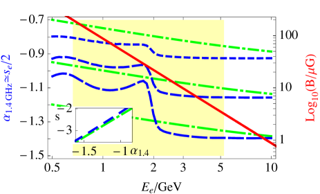
Figure 3.— The relation between $\alpha$ (dashed curves; left axis), $B$ (solid curve, right axis) and $E_{e}$ (abscissa), for $\nu_{e}=1.4\mbox{ GHz}$. The highly magnetized, $B_{cmb}(z=0)<B<200\mbox{ $\mu$G}$ regime is shaded. The radio spectral index $\alpha_{1.4}$ is shown as a function of $E_{e}$ according to model A (dashed) and model B (dash-dotted), for CRP spectral indices $s=-2$, $-2.5$, and $-3$ (top to bottom). See §5.2 for model and parameter description. Inset: The CRP energy index $s$ as a function of radio spectral index $\alpha_{1.4}$ for $B=B_{cmb}$ (for example, at the spatial halo break; see §5.1).

Due to the limited energy range over which the energy index $s_{e}\equiv d\log(n_{e})/d\log(E_{e})$ of the injected CREs can be computed, the radio spectrum in Fig. 3 is calculated in the approximation where each CRE emits a single photon, such that $\alpha\simeq s_{e}/2$ (e.g., Keshet et al., 2003). A more accurate computation, convolving the CRE distribution with the synchrotron emission function, would somewhat smear the spectral features.

The radio steepening with increasing $E_{e}$ implies steepening with increasing $\nu$ or $r$, or decreasing $T$, as observed. Both models agree that spectral steepening by $|\Delta\alpha_{\nu}|>0.2$ indicates $B>20(\nu_{e}/1.4\mbox{ GHz})\mbox{ $\mu$G}$ magnetic fields in the region associated with a flatter radio spectrum. Measuring $\alpha$ across the $E_{e}\simeq 2\mbox{ GeV}$ spectral break can be used to unambiguously fix the CRP spectrum $s$. Similarly, measuring $\alpha$ at the spatial ${\eta}$ break where $B\simeq B_{cmb}$ can be used to determine $s$, as illustrated in the inset of Fig. 3. Conversely, if a distinct spectral break exists as predicted by model A, it would directly gauge the magnetic field, once the CRP spectrum has been determined. Multi-frequency radio data could thus allow a sensitive mapping of the magnetic field, both above and below $B_{cmb}$, throughout the halo, using, for example, deprojected maps at several radio frequencies.

Spectral measurements of radio halos should be interpreted with caution. Contamination by CRE sources such as shocks, relics, central AGNs, and radio galaxies, is common. Spatial averaging often blends together different sources, depending on flux sensitivity and angular resolution. Therefore, with present observations, the spectrum can be reliably associated with a halo only when measured locally in uncontaminated regions; in our model these are regions of uniform ${\eta}$. Also note that radio emission above 1 GHz is increasingly suppressed by the Sunyaev-Zel’dovich effect (Enßlin, 2002).

For example, ${\eta}(r)$ is nearly constant in A665 within the range $r<r_{max}\simeq 150^{\prime\prime}$ examined in Fig. 2. Spectral steepening with increasing $r$ was identified in this cluster (Feretti et al., 2004b) by comparing radio maps at $0.3$ and $1.4\mbox{ GHz}$ frequencies. The spectral index steepens from $\alpha\simeq-1.0$ in the halo’s center to $\alpha\simeq-1.3$ towards the South and towards the East, within the flat ${\eta}$ region. Similar steepening was found towards the North and West beyond $r_{max}$, but the spectrum first flattens to $\alpha\simeq-0.9$.

Similarly, the regular GH in A2744 exhibits a linear radio-X-ray correlation in brightness out to $r\simeq 1\mbox{ Mpc}$ (Govoni et al., 2001a). Along the main NW elongation, the $0.3-1.4\mbox{ GHz}$ spectral slope $\alpha(r<200\mbox{ kpc})\simeq-1.0$, slightly flattens to $-0.9$ around $500\mbox{ kpc}$, and steepens again to $-1.5$ as $r\to 1\mbox{ Mpc}$. An azimuthal average, however, includes a NE relic tail and under-threshold regions, leading to an unrealistically uniform $\alpha(r<\mbox{Mpc})\simeq-1$ (Orrú et al., 2007). A similar behavior is found in A2219 (Orrú et al., 2007).

In these examples, the spectral index steepens with increasing $r$ from $\alpha\simeq-1.0$ to $-(1.2$-$1.5)$ in the less perturbed/contaminated direction, sometimes after a mild flattening to $\alpha\simeq-0.9$. Such steepening was also reported in A2163 (Feretti et al., 2004b) and in Coma (Giovannini et al., 1993).

Comparable steepening was found as a function of frequency in the GH in A754. Its spectrum measured between $74$ and $330\mbox{ MHz}$, $\alpha_{0.07}^{0.3}\sim-1.1$, steepens to $\alpha_{0.3}^{1.4}\sim-1.5$ (Bacchi et al., 2003). More substantial steepening has been reported in other clusters, such as A2319 (Feretti et al., 1997) and A3562 (Giacintucci et al., 2005). However, contamination by extended radio galaxies was reported in these halos.

Significant steepening with increasing $r$ or $\nu$ as in the examples above is more consistent with the $E_{e}\sim 2\mbox{ GeV}$ spectral break of model A than with model B. In model A, strong magnetic fields with $B\gtrsim 10(\nu_{e}/700\mbox{ MHz})\mbox{ $\mu$G}$ are present in regions where $\alpha_{\nu}$ is flat. Moreover, an uncontaminated spectral break measured at some emitted frequency $\nu_{b}$ would imply that the local projected magnetic field is $B\simeq 10(\nu_{b}/700\mbox{ MHz})\mbox{ $\mu$G}$. Observations at several frequencies can thus be used to map the local projected magnetic field. As a preliminary example, interpreting the radio spectrum of A754 as a spectral break somewhere between $\nu_{e}=200$ and $900\mbox{ MHz}$ near the center of the halo, would imply $3<B_{0}/{\mu\mbox{G}}<14$.

Figure 3 indicates that radio steepening from $\alpha=-1.0$ to $-1.3$ corresponds to a CRP spectral index $s\simeq-2.7$. Steepening beyond $-1.5$, if uncontaminated, would imply a steep CRP spectrum with $s<-3$. The radio spectrum at high, $E_{e}\gg 10\mbox{ GeV}$ CRE energies approaches $\alpha\to s/2$. However, inward of the spectral break, at $E_{e}<2\mbox{ GeV}$, $\alpha\simeq-1$ depends only weakly on $s$. This could explain the universally observed $\alpha\simeq-1$ in the centers of halos.

Figure 4 shows the average $\nu\lesssim 1.4\mbox{ GHz}$ spectral indices $\langle\alpha_{1.4}\rangle$ reported for GHs in our sample, as a function of their minimal central magnetic fields $B_{0,min}$ calculated in §5.1. The results are also summarized in Table 1. A positive correlation is seen, in the sense that halos with stronger central magnetization tend to have a flatter radio spectrum, as expected. Note that this correlation is stronger than, and not simply due to, a correlation we find between $\langle\alpha\rangle$ and the halo size.

For comparison, we also plot (dashed lines in Fig. 4) the average radio spectrum $\langle\alpha_{1.4}\rangle$ as a function of $B_{0}$, computed for a typical isothermal $\beta$-model with $\beta=0.7$, assuming $B^{2}\propto nT$, spectral model A, and radio emission extending to $R_{\nu}\simeq 3r_{c}$. Although this result cannot be quantitatively compared to the GH data (which are only lower limits on $B_{0}$), the trends qualitatively agree. This provides an independent indication that the CRP spectrum is steep, with $s\lesssim-2.7$.

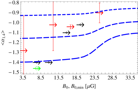
Figure 4.— The relation between the spatially averaged, $\nu\lesssim 1.4\mbox{ GHz}$ spectral index $\langle\alpha_{1.4}\rangle$, and the central magnetic field $B_{0}$. The measured spectral index in each GH is plotted as a function of the minimal central magnetic field $B_{0,min}$ calculated in §5.1 (right arrows; data with no reported error bars shown as diamonds; data with error bars larger than the y-axis shown as a circle; see Table 1). Also shown (dashed curves) is the average spectrum calculated in a simple magnetic equipartition, isothermal $\beta$-model (see §5.2), as a function of the central magnetic field, for CRP energy indices $s=-2$, -2.5, and -3 (top to bottom).

The radio spectrum is relatively steep in the five GHs and MHs for which we presented evidence for low magnetization in §5.1, in agreement with the $\langle\alpha\rangle-B_{0}$ correlation. The halos which are not shown in Fig. 4, include A2029 ($\langle\alpha_{0.2}\rangle\simeq-1.35$, Slee & Siegman, 1983), A2255 ($\langle\alpha_{0.3}^{1.4}\rangle=-2.06\pm 0.57$, Kempner & Sarazin, 2001, where we infer $\langle\alpha_{0.6}^{1.4}\rangle\sim-1.5$ by comparing M09 with Harris et al. (1980)), Perseus ($\langle\alpha_{0.3}^{1.5}\rangle\sim-1.2$, Gitti et al., 2004), and RXC J2003.5 -2323 ($\langle\alpha_{0.2}^{1.4}\rangle\sim-1.32\pm 0.06$, Giacintucci et al., 2009).

Finally, a cautionary comment is in place regarding the extrapolation of the spectrum to low frequencies that correspond to $E_{e}\lesssim 1\mbox{ GeV}$ CRE energies. Although $E_{e}=1\mbox{ GeV}$ CREs are produced on average by $E_{p}\sim 20\mbox{ GeV}$ CRPs (for $s=-2.5$), the contribution of low energy CRPs with $E_{p}\lesssim 3\mbox{ GeV}$ is not negligible. We expect a CRP power law energy spectrum $n_{p}(E_{p})\propto E_{p}^{s}$ to be modified around the proton rest mass. Consequently, our $s=\mbox{constant}$ approximation becomes increasingly unlikely at low, $E_{e}\lesssim\mbox{few}\mbox{ GeV}$ CRE energies.

6. Discussion: origin of CRIs and magnetic fields

In the previous sections we studied the luminosity (in §2) and the surface brightness (in §3) properties of GHs and MHs, showed that they are best explained by a model invoking secondary CREs and strong magnetic fields as the source of radio halos (in §4), and discussed some implications of such a model (in §5). Here we consider the origins of the magnetic fields (§6.1) and of the primary CRIs (§6.2). We subsequently summarize our work in §6.3.

6.1. Magnetization: mergers (GHs) and sloshing (MHs)

In the model derived above, the primary CRI population is long-lived and has very similar properties in different clusters and in different parts of a cluster. Hence, the defining property of halos is sufficiently high magnetization. Measuring strong, $B>B_{cmb}$ magnetic fields without radio detection at the level given by Eq. (4) would rule out the model, unless the CRI energy fraction is exceptionally low (e.g., due to a low level of star formation; see §6.2). The model can be tested by checking if the different magnetic field estimates it produces in a given halo are self consistent, and agree with independent measurements.

In the model, GH clusters are associated with strong, $B\gtrsim B_{cmb}\sim 3\mbox{ $\mu$G}$ magnetic fields, whereas weaker, $B<B_{cmb}$ fields are present in clusters devoid of a halo. Magnetic fields of the order of $B_{cmb}$, extending over Mpc scales, are consistent with Faraday rotation measures (RM) in non-cool clusters, considering the uncertainties involved. Such RM studies suggest magnetic fields ranging between a few $\mu$G to $10\mbox{ $\mu$G}$, extending out to $r\sim 500\mbox{ kpc}$, in a sample of non-cool core clusters, on $10$–$20\mbox{ kpc}$ coherence scales (Clarke, 2004). Weaker magnetic fields, typically $\sim 1\mbox{ $\mu$G}$ to a few $\mu$G, were found using other methods, such as simulating the polarization of extended sources (Murgia et al. 2004) or using a Bayesian maximum likelihood analysis of the Faraday RM (Vogt & Enßlin, 2005).

RM studies could potentially test the association between strong magnetization and the presence of halos, as implied by the model, although this is complicated by several factors. First, RM analyses involve substantial systematic and statistical errors associated with projection effects, the magnetic power spectrum, the range of coherence scales, and non-Gaussianity. Second, cluster fields are often reconstructed using peripheral RM sources, assuming some magnetic field scaling $B\propto n^{\mu}$ that extends both inside and outside the halo; however this assumption is uncertain and in some cases inconsistent with our model, e.g., in asymmetric or clumpy halos. Finally, the RM gauges the magnetic field amplitude integrated along the line of sight, whereas the radio emission scales differently with the magnetic field, e.g., as $B^{2}$ in $B\lesssim B_{cmb}$ regions.

It is interesting to compare the magnetic fields estimated in different clusters. Care must be taken to compare the same measures estimated under the same assumptions. For example, assuming a Gaussian, Kolmogorov magnetic power spectrum with $\mu=1/2$, we find ${\langle{B(r<3r_{c})}\rangle}=1.8\mbox{ $\mu$G}$ and $B(3r_{c})=1.3\mbox{ $\mu$G}$ in Coma (Bonafede et al., 2010), which harbors a GH, while weaker fields, ${\langle{B(r<3r_{c})}\rangle}=1.2\mbox{ $\mu$G}$ and $B(3r_{c})=0.8\mbox{ $\mu$G}$ are found in A2382 (Guidetti et al., 2008), which has no halo. Similarly, ${\langle{B(r<3r_{c})}\rangle}=1.3\mbox{ $\mu$G}$ and $B(3r_{c})=0.8\mbox{ $\mu$G}$ are found in A119 (Murgia et al., 2004), which does not harbor a GH, but this result is obtained for $\mu=0.9$ so comparison to the other two clusters may be misleading. Note that it is not clear, considering the inherent uncertainties, if the differences between these $B$ estimates are significant.

The association between GHs and merger events is fairly well established (see Feretti & Giovannini, 2008, and references therein). With present magnetic field estimates, it is quite plausible that a major merger event could amplify the intracluster magnetic field by a factor of a few, sufficient to exceed $B_{cmb}$ and produce a GH. The model thus resolves the notorious discrepancy between magnetic field estimates based on Faraday RM and on previous GH analyses, which unnecessarily assumed equipartition between magnetic fields and CREs.

The very strong magnetic fields we infer in the centers of MHs are consistent with the RM observed in CCs, which typically imply $B\simeq 10-40\mbox{ $\mu$G}$ in the core, on coherence scales of a few up to $10\mbox{ kpc}$ (Carilli & Taylor, 2002). It is interesting to point out that the cooling flow power is correlated both with the RM (Taylor et al., 2002) and with the MH radio power (Gitti et al., 2004), while no strong correlation between MH and AGN power was identified (e.g., Govoni et al., 2009).

The association between MH edges and CFs strongly suggests that sloshing motions play a major role in magnetizing the core. Notice that $\sim 10\mbox{ kpc}$ scales are indeed characteristic of the shear magnetic amplification anticipated beneath CFs (Keshet et al., 2010). Sloshing could suppress cooling in the core, for example by mixing the cold gas with a heat inflow (Markevitch & Vikhlinin, 2007). In such a scenario, a stronger cooling flow may correspond to a larger magnetized region, leading to correlations between the cooling flow power and both RM and MH power, as observed, but not necessarily to an MH-AGN correlation.

The distribution of MHs (without the AGN component) among CCs should reflect the statistics of core magnetization, and therefore of sloshing. We expect a correlation between the presence of MHs and of CFs in a cluster, and a correlation between the MH size or power and the shear flow strength, manifest for example in the number and size of CFs and in the (measurable, see Keshet et al., 2010) shear across them. Assuming that some level of magnetization by core sloshing is always present in CCs, as suggested by the ubiquity of observed CFs, the steep magnetic profile associated with the density cusp would imply that every CC has some MH, even if small. The MH distribution would then be continuous, and not bimodal as in GHs.

Shear amplification of magnetic fields parallel to the CF plane is expected mostly below the CF and in a thin boundary layer around it, in which the field can reach high, near equipartition levels (Keshet et al., 2010). The morphological association between MH edges and CFs, discovered by Mazzotta & Giacintucci (2008), is therefore expected to be ubiquitous. It is best seen where CFs are observed edge on; elsewhere it may be observed as morphological correlations between radio maps and spatial X-ray gradients, which trace projected CFs.

The magnetic field (the polarization) is expected to be parallel (perpendicular) to the CF, i.e. approximately tangential (radial). Polarization would be preferentially observable where beam deprojection is minimal, i.e. at large radii where the magnetic field weakens. Interestingly, nearly radial, $10\%-20\%$ polarization was detected in the MH in A2390, growing stronger with increasing radius (we refer to the spherical, $r\sim 150\mbox{ kpc}$ component around the cD galaxy in this irregular MH; see Bacchi et al., 2003). We predict that near CF edges, where the magnetic field is particularly strong, the radio spectrum would be relatively flat (see §5.2).

6.2. CRI Origin: diffusion and supernovae sources

The spectral steepening of the radio signal with increasing CRE energy $E_{e}\propto(\nu/B)^{1/2}$, provides a novel method for measuring the primary CRP spectrum. The radio steepening observed in some halos, roughly from $\alpha\simeq-1.0$ to $\alpha\simeq-1.3$, corresponds to a CRP spectral index $s\lesssim-2.7$ at $E_{p}\sim 20\mbox{ GeV}$ energies. The CRP energy fraction then becomes (cf. Eq. 10)

$$\xi_{p}(>E_{p}) \equiv \frac{u_{p}(>E_{p})}{u_{th}}\simeq 10^{-3.6\pm 0.2}\left(\frac{E_{p}}{10\mbox{ GeV}}\right)^{-0.7}\mbox{ .}\,\,\,\,$$ (14)

Note that with the uncertain and possibly contaminated radio spectra presently available, a steeper CRP spectrum with $s\simeq-3$ is possible. The model would be challenged if the uncontaminated spectrum of a substantial halo population turns out to be much steeper than $\alpha=-1.5$, unless the corresponding steep CRP spectrum can be explained.

The CRP distribution in Eq. (14) resembles (but has an energy fraction a few $100$ times smaller than) the CRP distribution found in the solar vicinity above $1\mbox{ GeV}/$nucleon. This distribution could originate from sources that inject roughly equal energy per decade of CRP energy ($s_{0}\simeq-2.2$), such as supernovae (SNe), if energy-dependent diffusion is significant in the inner halo regions. For example, a simple estimate of CRI scattering off magnetic irregularities with a Kolmogorov power spectrum yields a diffusion coefficient $D\simeq 10^{30}(E_{p}/\mbox{GeV})^{1/3}(B/\mu\mbox{G})^{-1/3}\mbox{ cm}^{2}\mbox{ s}^{-1}$ (Völk et al., 1996). This implies CRI diffusion over $\sim 0.5\mbox{ Mpc}$ during a Hubble time, and a steepening by $\Delta s=-1/2$. More substantial steepening is possible if the diffusion function has a stronger energy dependence. For example, the diffusion function is often assumed to scale as $D\propto E_{p}^{1/2}$, which could lead to a $\Delta s=-3/4$ steepening in the CRI spectrum.

The CRI output of SNe can be crudely estimated (Völk et al., 1996) if we assume that a fraction $f_{\mbox{\scriptsize{II}}}$ of the cluster’s $Z=0.3Z_{0.3}$ solar metallicity is seeded by Type II SNe, which on average produce $0.1M_{\odot}M_{Fe,0.1}$ of iron and deposit a fraction $\xi=0.3\xi_{0.3}$ of the $10^{51}E_{51}\mbox{ erg}$ explosion energy in $E_{p}>10\mbox{ GeV}$ CRIs,

$$\xi_{p}^{SN}\simeq 0.03f_{\mbox{\scriptsize{II}}}Z_{0.3}E_{51}M_{Fe,0.1}^{-1}\xi_{0.3}\mbox{ .}$$ (15)

This can reproduce Eq. (14) if over the cluster’s lifetime, the CRIs diffuse to distances a few times larger than the radius $R_{\nu}$ of the radio halo. Note that if CRI diffusion is entirely absent, the CRIs accelerated in SNe would be confined to the cluster, and adiabatic losses could only lower their energy density to the level of Eq. (14). However, they would then retain their flat, $s\simeq-2.2$ spectrum.

An SNe origin of CRIs can be tested by examining the correlations between ${\eta}$ and (intensive) tracers of SNe activity among different halos. One possible tracer is the local metallicity measured at $r=0.1r_{500}$, tabulated in Table 1. We chose to use $Z(0.1r_{500})$ because (i) it was measured for all the M09 halos with XMM-Newton profiles in Snowden et al. (2008); (ii) the spatially averaged $Z$ is not meaningful when temperature gradients are large; and (iii) $0.1r_{500}$ lies well within the $Z(r>0.02r_{500})\propto r^{-0.3}$ decline typically found in both cool and non-cool core clusters (Sanderson et al., 2009). While our sample is statistically small, Perseus, which shows a significantly higher ${\eta}$ than in all the other halos in our sample, also shows a slightly higher $Z(0.1r_{500})$ (Snowden et al., 2008). However, due to the large uncertainty in abundance measurements, the elevated metallicity in Perseus is not significant ($<1\sigma$) with respect to some halos. Moreover, at smaller radii $r\lesssim 0.025r_{500}$, the metallicity in A2029 appears to be higher than in all other halos, and is significantly ($>3\sigma$) higher than in Perseus (Snowden et al., 2008).

Although better metallicity statistics may identify a more significant correlation between ${\eta}$ and $Z$, metallicity is probably not the most useful tracer of the SNe contribution to CRIs in the halo. Metallicity provides a cumulative measure of SNe activity, tracing the metals released from all past SNe in the cluster. In a model where a significant fraction of the CRIs have already diffused away from the cluster’s center, metallicity would not linearly trace the population of CRIs residing within the halo, especially in the more compact MHs. It is more appropriate to use an intensive tracer of recent SNe activity, such as the star formation rate (SFR) normalized by the cluster’s gas mass $M_{g}$, or the fraction of star forming galaxies. A correlation between an SNe measure and a CRI tracer, such as ${\eta}$ or the deviation from the luminosity correlation $\nu P_{\nu}/\bar{L}_{X[0.1,2.4]}^{1.7}$, may be more useful than the metallicity in establishing or ruling out an SNe origin of halo CRIs.

As seen in Fig. 2, the halos with the highest ${\eta}$ in our sample are the MH in Perseus and the GH in A665, while the halos with the lowest ${\eta}$ are the MH in A2029 and the GH in A773. Interestingly, the literature shows evidence for exceptionally high specific star formation in both Perseus and A665, and for a low specific SFR in A2029. (We found no relevant data for A773.)

In Perseus, which has the smallest $M_{g}$ (by at least a factor of $4$, see Fukazawa et al., 2004) and one of the most powerful cooling flows within our sample (e.g., White, 2000; Allen et al., 2002), there is optical-to-UV evidence for a relatively high SFR (e.g., Bregman et al., 2006; Rafferty et al., 2008). In particular, the cD galaxy NGC1275 in Perseus has a high SFR of $\sim 30M_{\odot}\mbox{ yr}^{-1}$ (Dixon et al., 1996) — the highest in our sample when normalized by $M_{g}$. Notice that the central galaxy in A1835 has a higher SFR of $\sim 100M_{\odot}\mbox{ yr}^{-1}$ — the highest SFR known in such objects (Peterson & Fabian, 2006). However, $M_{g}$ is $\sim 10$ times larger in A1835 with respect to Perseus (Fukazawa et al., 2004). Note that regions containing a high density of cosmic-rays are directly observed in Perseus in the form of X-ray cavities, reaching distances $r>100\mbox{ kpc}$ (M. Markevitch, private communications). A high specific SFR is also inferred in A665, which was found to be the cluster with the highest dispersion in color magnitude relation (a known tracer of star formation) in a sample of 57 X-ray bright clusters (López-Cruz et al., 2004). In contrast, A2029 has a low specific SFR, as it was shown to have a SFR $\sim 70$ times lower than in A1835 (Hicks & Mushotzky, 2005) while its gas mass is only $\sim 1.8$ times smaller (Fukazawa et al., 2004).

While these trends support an SNe origin of CRIs, more work is needed in order to quantify their significance and compile a comparative statistical analysis. Note that the combination of a strong correlation of ${\eta}$ with the specific SFR and a poor correlation with metallicity, if established, would directly imply that CRI diffusion is significant. Indeed, it is difficult to explain the steep, $s\lesssim-2.7$ spectrum without invoking CRI diffusion.

The above estimates of diffusive steepening assume that most of the CRIs produced by the sources presently dominating the halo have already escaped beyond it. This is consistent with the typical SFR peak at $z\sim 1$, and with the above estimates of the halo CRI abundance and the total CRI output of SNe (cf. Eqs. 14 and 15). However, such substantial diffusion would introduce some scatter in the radio–X-ray correlation, depending on the CRI production history of each cluster. Quantitative estimates of the SNe history of GH clusters, needed to compute this scatter, are beyond the scope of this work.

6.3. Summary and Conclusions

We have shown that the radio-X-ray correlation in GH luminosity (Eq. 1) can be generalized (Eq. 2) to hold for both GHs and MHs (Fig. 1), by correcting for the halo size. A universal, linear relation between the radio and X-ray surface brightness, $\eta=10^{-4.4\pm 0.2}$, was presented (Eq. 4 and Fig. 2). This, combined with the radial ${\eta}$ and $T$ profiles, implies a universal radio emissivity $\nu j_{\nu}=10^{-31.4\pm 0.2}n_{-2}^{2}(T/T_{0})^{0.2\pm 0.5}\mbox{ erg}\mbox{ s}^{-1}\mbox{ cm}^{-3}$ (Eq. 7) near the center of halos. We argued that these results and their applicability to GHs and MHs alike, strongly support one model for all halos, involving secondary CREs (injected according to Eq. 10) and strong magnetic fields with $B\gtrsim B_{cmb}$, while disfavoring other models (Table 2).

This model makes useful predictions without requiring additional assumptions or fine tuning. Radio emission rapidly fades in regions where $B$ drops below $B_{cmb}$, producing a distinct radial break (e.g., in A2029 and in Perseus; Fig 2) or a clumpy/filamentary radio morphology (e.g., in RXC J2003.5 -2323, A2255, and A2319) that can be used to map $B\simeq B_{cmb}$ contours. Marginally magnetized regions with $B\lesssim B_{cmb}\propto(1+z)^{2}$ are characterized by relatively high polarization and a steeper radio spectrum; their morphology traces the magnetic evolution and can potentially reveal a temporal signal. We expect a higher incidence rate of such transition regions at higher redshift, while no halos should exist at very high redshift.

Another direct consequence of the model is radio spectral steepening with increasing $E_{e}^{2}\propto\nu/B$ (Eq. 13), i.e. with increasing $r$ or $\nu$ or decreasing T, as indeed is observed. Such steepening, and in particular a $B\simeq 10(\nu_{e}/700\mbox{ MHz})\mbox{ $\mu$G}$ spectral break (Fig. 3), gauges the magnetic field, roughly producing an additional $B$ contour for each radio map frequency. The spectral break could be used to accurately map $B$ throughout the halo, using future radio telescopes such as the Murchison Widefield Array (MWA), the LOw Frequency ARray (LOFAR), and SKA.

A pressure model can be used to extrapolate $B$ throughout the cluster. This indicates central magnetic fields $B_{0}$ (Eq. 12) that exceed $10\mbox{ $\mu$G}$ in most halos (see Table 1 for lower limits $B_{0,min}$). A correlation between the average radio spectral index $\langle\alpha\rangle$ and $B_{0}$, implied by the model, was identified in GH data (Fig. 4).

In our model, any source of strong ($B\gtrsim B_{cmb}$), persistent magnetic fields in the intracluster medium would have similar properties to radio halos, as long as it does not significantly inject additional cosmic rays. This may include some extended radio galaxies, which were recently found to exhibit properties similar to halos (Rudnick & Lemmerman, 2009). Conversely, the universal value of ${\eta}$ we predict for any highly magnetized, uncontaminated region in the intracluster medium provides a powerful test of the model.

The spectral steepening of the radio signal, the universality of $\alpha\simeq-1$ in the centers of halos, and the correlation between $\langle\alpha\rangle$ and $B_{0,min}$ (Fig. 4), indicate a steep CRI spectrum, $s\lesssim-2.7$, and thus favor significant CRI diffusion. In a diffusion model, the most plausible source of the CRIs (Eq. 14) is SNe (e.g., Eq. 15). We show (in §6.2) preliminary evidence for a correlation between ${\eta}$ and the SFR normalized by the gas mass $M_{g}$, supporting an SNe CRI origin. None of these properties is expected in an alternative model (K09), in which the secondary CREs arise from $\sim 1\mbox{ GeV}$ CRPs, which are accelerated in the cluster’s virial shock and advected inward with the flow, thus being compressed to $\sim 10\mbox{ GeV}$ energies. Note that the data slightly favors a $j_{\nu}\propto n^{2}T^{0}$ scaling within each cluster (see §4), which is natural if CRIs originate in SNe, rather than the $j_{\nu}\propto n^{2}T^{1}$ behavior anticipated if they are accelerated in the virial shock. Also note that adiabatic compression of CRIs produced at the virial shock and advected with the gas would lead to a radially increasing, ${\eta}\propto n^{-1/3}$ profile (due the soft equation of state of relativistic particles), which is not observed (see Fig. 2).

We stress that although our model and the model of K09 disagree regarding the origin of CRIs, the CRI distribution, the spectral properties of halos, and the role of diffusion, we reach the same conclusions regarding the radio mechanism: emission from secondary CREs in strong magnetic fields. This conclusion is based on (i) the tight radio-X-ray correlation in total GH luminosity and the GH bimodality (K09); (ii) the tight radio-X-ray correlation in both coincident luminosity and surface brightness, in both GHs and MHs, despite their different physical properties; (iii) the strong magnetic fields inferred from Faraday RMs in MHs and possibly (see §6.1) also in GHs; (iv) the tightening of the brightness correlation at small radii, away from merger shocks, radio relics, and their associated turbulence; (v) the $j_{\nu}\propto n^{2}T^{{\kappa}}$ scaling of the radio emissivity within each halo, where ${{\kappa}}\lesssim 1$; (vi) the coincidence between MH edges and CFs, manifest as a sharp radial cutoff in ${\eta}$ (e.g., in Perseus); (vii) a power-law radial break where ${\eta}(r\ll r_{b})\simeq\mbox{constant}$ and $\eta(r\gg r_{b})\propto B^{2}$, possibly seen in the MHs in A2029, A1835 and RXJ1347, and in the GH in A2319; (viii) the clumpy/filamentary morphology of some halos, where independent evidence for low magnetization is present; (ix) the spectral steepening and the correlation between $\langle\alpha\rangle$ and $B_{0}$ (this suggests strong magnetization provided that the CRI spectrum is steep, $s\lesssim-2.7$).

Each aspect of our model can be tested in the near future. The association between the presence of halos and strong, $B\gtrsim B_{cmb}$ magnetic fields can be directly tested by comparing the magnetization levels independently estimated in halo and in non-halo clusters, as illustrated in §6.1. The secondary origin of the halos can be tested if the CRIs are detected directly through their $\pi^{0}$ production; for example, such a detection of a CRI component substantially stronger than in Eq. (14) would rule out our model. The SNe origin of the CRIs can be tested by carefully examining the correlation between a CRI measure such as $\eta$, and an intensive SNe tracer such as the specific SFR, in a sample of halo clusters.

References

- Allen et al. (2002) Allen, S. W., Schmidt, R. W., & Fabian, A. C. 2002, MNRAS, 335, 256
- Allen et al. (2003) Allen, S. W., Schmidt, R. W., Fabian, A. C., & Ebeling, H. 2003, MNRAS, 342, 287
- Anderson et al. (2009) Anderson, M. E., Bregman, J. N., Butler, S. C., & Mullis, C. R. 2009, ApJ, 698, 317
- Andersson et al. (2009) Andersson, K., Peterson, J. R., Madejski, G., & Goobar, A. 2009, ApJ, 696, 1029
- Arnaud (1996) Arnaud, K. A. 1996, in Astronomical Society of the Pacific Conference Series, Vol. 101, Astronomical Data Analysis Software and Systems V, ed. G. H. Jacoby & J. Barnes, 17–+
- Ascasibar & Markevitch (2006) Ascasibar, Y. & Markevitch, M. 2006, ApJ, 650, 102
- Augusto et al. (2006) Augusto, P., Edge, A. C., & Chandler, C. J. 2006, MNRAS, 367, 366
- Bacchi et al. (2003) Bacchi, M., Feretti, L., Giovannini, G., & Govoni, F. 2003, A&A, 400, 465
- Baldi et al. (2007) Baldi, A., Ettori, S., Mazzotta, P., Tozzi, P., & Borgani, S. 2007, ApJ, 666, 835
- Blattnig et al. (2000) Blattnig, S. R., Swaminathan, S. R., Kruger, A. T., Ngom, M., & Norbury, J. W. 2000, Phys. Rev. D, 62, 094030
- Böhringer et al. (2000) Böhringer, H., Voges, W., Huchra, J. P., McLean, B., Giacconi, R., Rosati, P., Burg, R., Mader, J., Schuecker, P., Simiç, D., Komossa, S., Reiprich, T. H., Retzlaff, J., & Trümper, J. 2000, ApJS, 129, 435
- Bonafede et al. (2009) Bonafede, A., Feretti, L., Giovannini, G., Govoni, F., Murgia, M., Taylor, G. B., Ebeling, H., Allen, S., Gentile, G., & Pihlström, Y. 2009, A&A, 503, 707
- Bonafede et al. (2010) Bonafede, A., Feretti, L., Murgia, M., Govoni, F., Giovannini, G., Dallacasa, D., Dolag, K., & Taylor, G. B. 2010, ArXiv e-prints
- Bonamente et al. (2006) Bonamente, M., Joy, M. K., LaRoque, S. J., Carlstrom, J. E., Reese, E. D., & Dawson, K. S. 2006, ApJ, 647, 25
- Bregman et al. (2006) Bregman, J. N., Fabian, A. C., Miller, E. D., & Irwin, J. A. 2006, ApJ, 642, 746
- Brunetti et al. (2009) Brunetti, G., Cassano, R., Dolag, K., & Setti, G. 2009, A&A, 507, 661
- Brunetti & Lazarian (2007) Brunetti, G. & Lazarian, A. 2007, MNRAS, 378, 245
- Brunetti et al. (2007) Brunetti, G., Venturi, T., Dallacasa, D., Cassano, R., Dolag, K., Giacintucci, S., & Setti, G. 2007, ApJ, 670, L5
- Carilli & Taylor (2002) Carilli, C. L. & Taylor, G. B. 2002, ARA&A, 40, 319
- Cassano et al. (2006) Cassano, R., Brunetti, G., & Setti, G. 2006, MNRAS, 369, 1577
- Cassano et al. (2007) Cassano, R., Brunetti, G., Setti, G., Govoni, F., & Dolag, K. 2007, MNRAS, 378, 1565
- Cassano et al. (2008) Cassano, R., Gitti, M., & Brunetti, G. 2008, A&A, 486, L31
- Cavaliere & Fusco-Femiano (1976) Cavaliere, A. & Fusco-Femiano, R. 1976, A&A, 49, 137
- Chen et al. (2007) Chen, Y., Reiprich, T. H., Böhringer, H., Ikebe, Y., & Zhang, Y. 2007, A&A, 466, 805
- Clarke (2004) Clarke, T. E. 2004, Journal of Korean Astronomical Society, 37, 337
- Dallacasa et al. (2009) Dallacasa, D., Brunetti, G., Giacintucci, S., Cassano, R., Venturi, T., Macario, G., Kassim, N. E., Lane, W., & Setti, G. 2009, ApJ, 699, 1288
- David et al. (1993) David, L. P., Slyz, A., Jones, C., Forman, W., Vrtilek, S. D., & Arnaud, K. A. 1993, ApJ, 412, 479
- Dennison (1980) Dennison, B. 1980, ApJ, 239, L93
- Dixon et al. (1996) Dixon, W. V. D., Davidsen, A. F., & Ferguson, H. C. 1996, AJ, 111, 130
- Enßlin (2002) Enßlin, T. A. 2002, A&A, 396, L17
- Enßlin et al. (1999) Enßlin, T. A., Lieu, R., & Biermann, P. L. 1999, A&A, 344, 409
- Feretti et al. (2004a) Feretti, L., Brunetti, G., Giovannini, G., Kassim, N., Orrú, E., & Setti, G. 2004a, Journal of Korean Astronomical Society, 37, 315
- Feretti et al. (2001) Feretti, L., Fusco-Femiano, R., Giovannini, G., & Govoni, F. 2001, A&A, 373, 106
- Feretti & Giovannini (2008) Feretti, L. & Giovannini, G. 2008, in Lecture Notes in Physics, Berlin Springer Verlag, Vol. 740, A Pan-Chromatic View of Clusters of Galaxies and the Large-Scale Structure, ed. M. Plionis, O. López-Cruz, & D. Hughes, 143–+
- Feretti et al. (1997) Feretti, L., Giovannini, G., & Bohringer, H. 1997, New Astronomy, 2, 501
- Feretti et al. (2004b) Feretti, L., Orrù, E., Brunetti, G., Giovannini, G., Kassim, N., & Setti, G. 2004b, A&A, 423, 111
- Ferrari et al. (2008) Ferrari, C., Govoni, F., Schindler, S., Bykov, A. M., & Rephaeli, Y. 2008, Space Science Reviews, 134, 93
- Fukazawa et al. (2004) Fukazawa, Y., Makishima, K., & Ohashi, T. 2004, PASJ, 56, 965
- Giacintucci et al. (2005) Giacintucci, S., Venturi, T., Brunetti, G., Bardelli, S., Dallacasa, D., Ettori, S., Finoguenov, A., Rao, A. P., & Zucca, E. 2005, A&A, 440, 867
- Giacintucci et al. (2009) Giacintucci, S., Venturi, T., Brunetti, G., Dallacasa, D., Mazzotta, P., Cassano, R., Bardelli, S., & Zucca, E. 2009, A&A, 505, 45
- Ginzburg & Syrovatsky (1961) Ginzburg, V. L. & Syrovatsky, S. I. 1961, Progress of Theoretical Physics Supplement, 20, 1
- Giovannini et al. (2009) Giovannini, G., Bonafede, A., Feretti, L., Govoni, F., Murgia, M., Ferrari, F., & Monti, G. 2009, A&A, 507, 1257
- Giovannini et al. (2003) Giovannini, G., Feretti, L., Bacchi, M., & Govoni, F. 2003, in ASP Conf. Ser. 301, Matter and Energy in Clusters of Galaxies, ed. S. Bowyer & C.-Y. Hwang (San Francisco, CA: ASP), 483
- Giovannini et al. (1993) Giovannini, G., Feretti, L., Venturi, T., Kim, K., & Kronberg, P. P. 1993, ApJ, 406, 399
- Gitti et al. (2004) Gitti, M., Brunetti, G., Feretti, L., & Setti, G. 2004, A&A, 417, 1
- Gitti et al. (2002) Gitti, M., Brunetti, G., & Setti, G. 2002, A&A, 386, 456
- Govoni et al. (2001a) Govoni, F., Enßlin, T. A., Feretti, L., & Giovannini, G. 2001a, A&A, 369, 441
- Govoni et al. (2001b) Govoni, F., Feretti, L., Giovannini, G., Böhringer, H., Reiprich, T. H., & Murgia, M. 2001b, A&A, 376, 803
- Govoni et al. (2004) Govoni, F., Markevitch, M., Vikhlinin, A., VanSpeybroeck, L., Feretti, L., & Giovannini, G. 2004, ApJ, 605, 695
- Govoni et al. (2005) Govoni, F., Murgia, M., Feretti, L., Giovannini, G., Dallacasa, D., & Taylor, G. B. 2005, A&A, 430, L5
- Govoni et al. (2009) Govoni, F., Murgia, M., Markevitch, M., Feretti, L., Giovannini, G., Taylor, G. B., & Carretti, E. 2009, A&A, 499, 371
- Guidetti et al. (2008) Guidetti, D., Murgia, M., Govoni, F., Parma, P., Gregorini, L., de Ruiter, H. R., Cameron, R. A., & Fanti, R. 2008, A&A, 483, 699
- Harris et al. (1980) Harris, D. E., Kapahi, V. K., & Ekers, R. D. 1980, A&AS, 39, 215
- Hicks & Mushotzky (2005) Hicks, A. K. & Mushotzky, R. 2005, ApJ, 635, L9
- Kaastra (1992) Kaastra, J. S. 1992, An X-Ray Spectral Code for Optically Thin Plasmas, Internal SRON-Leiden Report, updated version 2.0
- Kamae et al. (2006) Kamae, T., Karlsson, N., Mizuno, T., Abe, T., & Koi, T. 2006, ApJ, 647, 692
- Kempner & Sarazin (2001) Kempner, J. C. & Sarazin, C. L. 2001, ApJ, 548, 639
- Keshet et al. (2010) Keshet, U., Markevitch, M., Birnboim, Y., & Loeb, A. 2010, ApJ, 719, L74
- Keshet et al. (2003) Keshet, U., Waxman, E., Loeb, A., Springel, V., & Hernquist, L. 2003, ApJ, 585, 128
- Kushnir et al. (2009) Kushnir, D., Katz, B., & Waxman, E. 2009, Journal of Cosmology and Astro-Particle Physics, 9, 24 (K09)
- Kushnir & Waxman (2010) Kushnir, D. & Waxman, E. 2010, Journal of Cosmology and Astro-Particle Physics, 2, 25
- Liedahl et al. (1995) Liedahl, D. A., Osterheld, A. L., & Goldstein, W. H. 1995, ApJ, 438, L115
- López-Cruz et al. (2004) López-Cruz, O., Barkhouse, W. A., & Yee, H. K. C. 2004, ApJ, 614, 679
- Macario et al. (2010) Macario, G., Venturi, T., Brunetti, G., Dallacasa, D., Giacintucci, S., Cassano, R., Bardelli, S., & Athreya, R. 2010, ArXiv e-prints
- Markevitch (1998) Markevitch, M. 1998, ApJ, 504, 27
- Markevitch & Vikhlinin (2007) Markevitch, M. & Vikhlinin, A. 2007, Phys. Rep., 443, 1
- Matsumoto et al. (2001) Matsumoto, H., Pierre, M., Tsuru, T. G., & Davis, D. S. 2001, A&A, 374, 28
- Matsumoto et al. (2000) Matsumoto, H., Tsuru, T. G., Fukazawa, Y., Hattori, M., & Davis, D. S. 2000, PASJ, 52, 153
- Mazzotta & Giacintucci (2008) Mazzotta, P. & Giacintucci, S. 2008, ApJ, 675, L9
- Mewe et al. (1985) Mewe, R., Gronenschild, E. H. B. M., & van den Oord, G. H. J. 1985, A&AS, 62, 197
- Mewe et al. (1986) Mewe, R., Lemen, J. R., & van den Oord, G. H. J. 1986, A&AS, 65, 511
- Morandi et al. (2007) Morandi, A., Ettori, S., & Moscardini, L. 2007, MNRAS, 379, 518
- Murgia et al. (2004) Murgia, M., Govoni, F., Feretti, L., Giovannini, G., Dallacasa, D., Fanti, R., Taylor, G. B., & Dolag, K. 2004, A&A, 424, 429
- Murgia et al. (2009) Murgia, M., Govoni, F., Markevitch, M., Feretti, L., Giovannini, G., Taylor, G. B., & Carretti, E. 2009, A&A, 499, 679 (M09)
- Norbury (2009) Norbury, J. W. 2009, Nuclear Instruments and Methods in Physics Research B, 267, 1209
- Orrú et al. (2007) Orrú, E., Murgia, M., Feretti, L., Govoni, F., Brunetti, G., Giovannini, G., Girardi, M., & Setti, G. 2007, A&A, 467, 943
- Peterson & Fabian (2006) Peterson, J. R. & Fabian, A. C. 2006, Phys. Rep., 427, 1
- Petrosian & Bykov (2008) Petrosian, V. & Bykov, A. M. 2008, Space Science Reviews, 134, 207
- Rafferty et al. (2008) Rafferty, D. A., McNamara, B. R., & Nulsen, P. E. J. 2008, ApJ, 687, 899
- Reiprich & Böhringer (2002) Reiprich, T. H. & Böhringer, H. 2002, ApJ, 567, 716
- Rephaeli et al. (2008) Rephaeli, Y., Nevalainen, J., Ohashi, T., & Bykov, A. M. 2008, Space Science Reviews, 134, 71
- Roland et al. (1981) Roland, J., Sol, H., Pauliny-Toth, I., & Witzel, A. 1981, A&A, 100, 7
- Rudnick & Lemmerman (2009) Rudnick, L. & Lemmerman, J. A. 2009, ApJ, 697, 1341
- Sanderson et al. (2009) Sanderson, A. J. R., O’Sullivan, E., & Ponman, T. J. 2009, MNRAS, 395, 764
- Santos et al. (2008) Santos, J. S., Rosati, P., Tozzi, P., Böhringer, H., Ettori, S., & Bignamini, A. 2008, A&A, 483, 35
- Schilizzi et al. (2007) Schilizzi, R. T., Alexander, P., Cordes, J. M., Dewdney, P. E., Ekers, R. D., Faulkner, A. J., Gaensler, B. M., Hall, P. J., Jonas, J. L., & Kellermann, K. I. 2007, Preliminary Specifications for the Square Kilometre Array, Kilometre Array collaboration document (2007), http://www.skatelescope.org/pages/page_astronom.htm
- Slee & Siegman (1983) Slee, O. B. & Siegman, B. C. 1983, Proceedings of the Astronomical Society of Australia, 5, 114
- Snowden et al. (2008) Snowden, S. L., Mushotzky, R. F., Kuntz, K. D., & Davis, D. S. 2008, A&A, 478, 615
- Taylor et al. (2002) Taylor, G. B., Fabian, A. C., & Allen, S. W. 2002, MNRAS, 334, 769
- Valtchanov et al. (2002) Valtchanov, I., Murphy, T., Pierre, M., Hunstead, R., & Lémonon, L. 2002, A&A, 392, 795
- van Weeren et al. (2009) van Weeren, R. J., Röttgering, H. J. A., Brüggen, M., & Cohen, A. 2009, A&A, 508, 75
- Vogt & Enßlin (2005) Vogt, C. & Enßlin, T. A. 2005, A&A, 434, 67
- Völk et al. (1996) Völk, H. J., Aharonian, F. A., & Breitschwerdt, D. 1996, Space Science Reviews, 75, 279
- White (2000) White, D. A. 2000, MNRAS, 312, 663
- Worrall & Birkinshaw (2003) Worrall, D. M. & Birkinshaw, M. 2003, MNRAS, 340, 1261
- Zhang et al. (2008) Zhang, Y., Finoguenov, A., Böhringer, H., Kneib, J., Smith, G. P., Kneissl, R., Okabe, N., & Dahle, H. 2008, A&A, 482, 451