The Sagittarius Dwarf Galaxy: a Model for Evolution in a Triaxial Milky Way Halo
Abstract
We present a new -body model for the tidal disruption of the Sagittarius (Sgr) dwarf that is capable of simultaneously satisfying the majority of angular position, distance, and radial velocity constraints imposed by current wide-field surveys of its dynamically young ( Gyr) tidal debris streams. In particular, this model resolves the conflicting angular position and radial velocity constraints on the Sgr leading tidal stream that have been highlighted in recent years. While the model does not reproduce the apparent bifurcation observed in the leading debris stream, recent observational data suggest that this bifurcation may represent a constraint on the internal properties of the Sgr dwarf rather than the details of its orbit. The key element in the success of this model is the introduction of a non-axisymmetric component to the Galactic gravitational potential which can be described in terms of a triaxial dark matter halo whose minor/major axis ratio and intermediate/major axis ratio at radii kpc. The minor/intermediate/major axes of this halo lie along the directions , , and respectively, corresponding to a nearly-oblate ellipsoid whose minor axis is contained within the Galactic disk plane. This particular disk/halo orientation is difficult to reconcile within the general context of galactic dynamics (and CDM models in particular), suggesting either that the orientation may have evolved significantly with time or that inclusion of other non-axisymmetric components (such as the gravitational influence of the Magellanic Clouds) in the model may obviate the need for triaxiality in the dark matter halo. The apparent proper motion of Sgr in this model is estimated to be mas yr-1, corresponding to a Galactocentric space velocity ) = (230, -35, 195) km s. Based on the velocity dispersion in the stellar tidal streams, we estimate that Sgr has a current bound mass . We demonstrate that with simple assumptions about the star formation history of Sgr, tidal stripping models naturally give rise to gradients in the metallicity distribution function (MDF) along the stellar debris streams similar to those observed in recent studies. These models predict a strong evolution in the MDF of the model Sgr dwarf with time, indicating that the chemical abundances of stars in Sgr at the present day may be significantly different than the abundances of those already contributed to the Galactic stellar halo. We conclude by using the new -body model to reevaluate previous claims of the association of miscellaneous halo substructure with the Sgr dwarf.
Subject headings:
galaxies: individual (Sagittarius) — Galaxy: structure — Galaxy: kinematics and dynamics — dark matter1. INTRODUCTION
With the advent of progressively deeper photometric surveys, it has become apparent that galactic haloes are threaded with the phase-mixed detritus of multiple generations of dwarf satellites that have been destroyed by the inexorable tides of their host’s gravitational potential. Surveys have indicated the presence of such streams in both the Milky Way (e.g., Majewski et al. 1996; Helmi et al. 1999; Newberg et al. 2002; Rocha-Pinto et al. 2004; Belokurov et al. 2006; Duffau et al. 2006; Grillmair & Dionatos 2006; Starkenburg et al. 2009) and other nearby galaxies (e.g., Shang et al. 1998; Ibata et al. 2001a; McConnachie et al. 2003; Kalirai et al. 2006; Martínez-Delgado et al. 2008, 2009), possibly constituting the primary source of the Galactic stellar halo (e.g., Searle & Zinn 1978; Majewski 1993, 2004; Majewski et al. 1996; Bullock et al. 2001b; Bullock & Johnston 2005; Font et al. 2006; Bell et al. 2008).
Perhaps the most prominent such stream is that from the Sagittarius dwarf spheroidal galaxy (hereafter Sgr dSph), whose lengthy tidal streams wrap entirely around the Milky Way. The first observations of Sgr were presented by Ibata et al. (1994), since which time significant observational effort has been invested in detecting and characterizing the stellar streams emanating from the dwarf. Observations of high-latitude carbon stars (Totten & Irwin 1998) and various small-field surveys (e.g., Dinescu et al. 2002, and references therein) fueled a host of early efforts to model the Sgr — Milky Way system by Johnston et al. (1995, 1999), Velazquez & White (1995), Edelsohn & Elmegreen (1997), Ibata et al. (1997), Gómez-Flechoso et al. (1999), Helmi & White (2001), Martínez-Delgado et al. (2004).
In the past seven years however, our understanding of the scope and significance of the streams has been revolutionized by the deep, wide-field views provided by the Two Micron All-Sky Survey (2MASS) and Sloan Digital Sky Survey (SDSS). In particular, the 2MASS survey showed a large population of young, relatively metal-rich Sgr M-giants wrapping or more across the sky (Majewski et al. 2003). SDSS observations have shown (Belokurov et al. 2006) that the debris streamer leading Sgr along its orbit continues to be well-defined through the North Galactic Pole as it passes over the solar neighborhood towards the Galactic anticenter. Follow-up spectroscopy (Majewski et al. 2004; Law et al. 2004; Yanny et al. 2009) has confirmed that the streams are similarly well-defined in radial velocity, and indicate a significant evolution in the metallicity distribution function (MDF) of the component stellar populations with increasing separation from the Sgr dwarf core along the tidal streams (e.g., Bellazini et al. 2006; Chou et al. 2007, 2009; Monaco et al. 2007; Starkenburg et al. 2009; Carlin et al. in prep.).
In the inner Galaxy, dynamical tracers such as tidal streams can provide strong constraints on the mass distribution of the baryonic components of the Milky Way (e.g., Font et al. 2001; Ibata et al. 2003; Koposov et al. 2009). At the larger radii kpc traced by the orbit of the Sgr dwarf however the gravitational potential is dominated by dark matter, and observations of the luminous tidal streams can be used to constrain the shape, orientation, and mass of the Milky Way’s dark halo (e.g., Ibata et al. 2001b; Helmi 2004; Johnston et al. 2005; Law et al. 2005 [hereafter LJM05]; Fellhauer et al. 2006; Martínez-Delgado et al. 2007). The breadth and quality of the recent observational data is such that it has highlighted a ‘halo conundrum’ (variously discussed by LJM05; Fellhauer et al. 2006; Martínez-Delgado et al. 2007; Newberg et al. 2007; and Yanny et al. 2009): In a static axisymmetric Milky Way dark halo no one model has been capable of simultaneously reproducing both the angular position and distances/radial velocities of tidal debris in the Sgr leading arm. Depending on which criterion a given study chose to focus, claims have been made in favor of an oblate halo (e.g., Johnston et al. 2005; Martínez-Delgado et al. 2007), an approximately spherical halo (e.g., Ibata et al. 2001b; Fellhauer et al. 2006), and a prolate halo (e.g., Helmi 2004).
As we demonstrated using massless test-particle orbits in Law, Majewski, & Johnston (2009; hereafter LMJ09) however, it is possible to resolve this conundrum by adopting a triaxial halo in which the minor axis is approximately aligned with the line of sight to the Galactic Center. In this contribution we extend the results of LMJ09 by performing detailed -body simulations of the tidal disruption of the Sgr dwarf within a range of Galactic halo parameterizations that were favored by test-particle orbits. In §2 we outline our basic numerical approach, describing the generalized form of the Milky Way — Sgr system along with an overview of the observational constraints on the Sgr tidal streams. We next describe our solution to the problem of constraining the basic orbital parameters of the Sgr stream (for a given Milky Way model) in §3, using these various simulations to discriminate between different realizations of the underlying Galactic potential in §4. The final parameters describing our best-fit model of the Milky Way — Sgr system are summarized in §5.
In §6 we discuss the best-fit model for the dark matter halo of the Milky Way that was derived in §4, and present possible theoretical challenges to, alternatives for, and methods of testing the triaxial halo model. We demonstrate in §7 that by adopting simple assumptions for the star formation history of Sgr it is possible to reproduce the trends in the MDF observed along the stellar tidal streams. We compare the best-fitting model of the Sgr streams to other observations of halo substructure that have previously been postulated to be associated with the Sgr stream in §8, and conclude in §9 with a summary of the successes and failures of our new model of the Milky Way — Sgr system and an overview of the key issues that need to be addressed in future work.
Throughout this paper we adopt the heliocentric Sgr coordinate system () defined by Majewski et al. (2003) in which the longitudinal coordinate in the direction of Sgr and increases along trailing tidal debris, and is positive towards the orbital pole .
2. Basic Approach
2.1. Numerical Framework
We adopt a basic formalism similar to that described by LJM05 and LMJ09. The Milky Way is described by a smooth fixed gravitational potential consisting of a Miyamoto-Nagai (1975) disk, Hernquist spheroid, and a logarithmic halo. The gravitational potential is therefore specified directly through the isovelocity ellipsoids both for consistency with previous studies and because these are more analytically accessible than working with an underlying mass distribution from which the gravitational acceleration must be numerically derived.
The respective contribution of these components is given by:
| (1) |
| (2) |
| (3) |
where are cylindrical/spherical radii respectively, and the various constants are given by
| (4) |
| (5) |
| (6) |
As discussed by LMJ09, this form for the dark halo potential describes an ellipsoid rotated by an angle about the Galactic axis, in which and are the axial flattenings along the equatorial axes and is the axial flattening perpendicular to the Galactic disk. We adopt the convention that corresponds to coincident with the Galactic axes respectively, and increases in the direction of positive Galactic longitude. Since only the ratios between the various are important (as increasing/decreasing in tandem is largely degenerate with the total halo mass normalization ), we fix .
We held fixed any parameter that was found not to be significantly constrained by Sgr (i.e., that did not significantly change the path of Sgr debris when varied). Following Johnston et al. (1999) and LJM05, we take , , kpc, kpc, and kpc. In LJM05 we explored the possibility of scaling the total mass of the Galactic disk through the parameter and found no compelling reason to adopt a value other than . We fix the distance to the Galactic Center to be kpc (e.g., Reid 1993; Groenewegen et al. 2008); in LJM05 we explored the possibility of varying , and found that for cases where the Sun lies approximately in the plane of the orbit (as is the case for Sgr) any reasonable choice of does not have a particularly noticeable effect on the quality-of-fit of our simulations. Additionally, Figure 4 of LJM05 suggests that the ideal choice of the scale length of the Galactic halo () is reasonably insensitive to the axial flattening adopted, and that a single fixed value of kpc should suffice. The normalization of the dark halo mass via the scale parameter is therefore entirely specified (for a given choice of , , and ) by the requirement that the speed of the Local Standard of Rest be km s. As for , is at present relatively unconstrained by observations of the Sgr stream (LJM05; although see discussion by Majewski et al. 2006; Carlin et al. in prep) and we simply fix to this conventional value. We note that if we were instead to adopt the proper motion of Sgr A∗ measured by Reid & Brunthaler (2004) it would imply km sfor our adopted value of kpc.
In a recent contribution (LMJ09) we integrated massless test-particles representing the Sgr dwarf along orbits in the Galactic potential defined by Eqns. 1 - 3 for a range111Note that LMJ09 only included the results from the range , in their Figures 3 and 4 since much of the , parameter space is degenerate with , . The non-degenerate parameter space with the minor axis oriented along was strongly disfavored in the LMJ09 simulations. of parameters , , . While the accuracy of such simple orbit models is necessarily limited because actual tidal debris from a massive satellite will deviate slightly from these orbits, LMJ09 were able to identify a region of parameter space around , , generally favorable to producing a model satellite capable of matching the observational constraints enumerated in §2.2. We note that while such test-particle orbits technically identify a second similarly acceptable region of parameter space around , , , the physical axis ratios of this region are degenerate with the first: Both have the short axis approximately aligned with the Galactic axis, and the longest with the Galactic . We choose to focus on the branch of the solution to avoid introducing degeneracy into our simulations.
Motivated by the successes of LMJ09, we perform -body simulations in Galactic models with a range of parameters , , . In each case, Sgr is integrated Gyr backwards in time along a simple test-particle orbit, and a -particle model for the dwarf is integrated forward again in time from this point to the present day. The particles in our model of Sgr are initially distributed to generate a Plummer (1911) model
| (7) |
where is the initial mass of Sgr and kpc is its scale length. We have assumed spherical symmetry and isotropy of the orbits within the initial Sgr dwarf since: 1) There is no evidence yet of significant rotation in the main body of the satellite, and 2) debris resulting from isotropic orbits will cover all phase-space regions accessible to non-isotropic satellites. The simulation particles are not associated with specific dark or light components, but instead trace the total mass of the satellite. The mutual interactions between these self-gravitating particles222The gravitational influence of the bound satellite is applied to all -body particles regardless of whether or not they are still bound to the dwarf. in the external Milky Way potential are calculated using a self-consistent field code (Hernquist & Ostriker 1992).
2.2. Overview of Observational Constraints
We summarize below the observational constraints that we adopt on the physical properties of the Milky Way — Sgr system, each of which is discussed in detail in §3 - 4. Generally, we have adopted these constraints because we consider them to be the strongest, most unambiguous available. Note that we opt not to constrain the model to match the apparent bifurcation in the Sgr leading arm described by Belokurov et al. (2006) since recent observational data presented by Yanny et al. (2009) suggest that feature may arise due to substructure within the Sgr dwarf rather than the shape of the Galactic gravitational potential (see discussion in §4.2 and 5.2).
While individual constraints are discussed in detail in §3, we summarize below
-
1.
Sgr must lie at the angular coordinates, distance, and radial velocity described in §3.1.
-
2.
Sgr must have a velocity vector that lies within the orbital plane defined by recent trailing tidal debris.
-
3.
The radial velocity dispersion among trailing tidal debris must match that observed by Monaco et al. (2007) using high resolution echelle spectroscopy.
-
4.
The run of radial velocities with orbital longitude along trailing tidal debris must match data presented by Majewski et al. (2004).
-
5.
The run of radial velocities with orbital longitude along leading tidal debris must match data presented by Law et al. (2004; see also LJM05).
-
6.
The angular location of leading tidal debris must match the high surface brightness stream observed by Belokurov et al. (2006) in the SDSS.
-
7.
The angular width of leading tidal debris must match that observed by Belokurov et al. (2006).
It turns out to be easiest to constrain the properties of the Sgr dwarf itself first (§3), since many of them are largely independent of the exact form of the Galactic potential (to within the range explored in this paper), and the rest may be constrained contingent upon a specific potential. We then use these simulations to discriminate between different realizations of the underlying Galactic potential in §4. We note that the only distance information explicitly incorporated in our fitting method is that used in setting the distance to the Sgr dwarf itself. Our analysis therefore relies only upon the most well-constrained observations of the tidal debris (namely, the angular coordinates and radial velocities) and is insensitive to photometric distance calibration uncertainties which have hindered confident interpretation of previous studies. While we do not fit for the distances to Sgr tidal debris explicitly, we shall see in §5 and §7.3 that the final model is nonetheless an excellent match to the distances derived for the observational data using the most reasonable assumptions about distance calibrations.
3. Constraining the Properties of the Sgr dSph
3.1. Core Properties
We assume that the Sgr dwarf is located at Galactic coordinates (Majewski et al. 2003). Estimates of the distance to Sgr typically range from kpc (see Table 2 of Kunder & Chaboyer 2009 for a summary); we adopt the distance scale kpc from Siegel et al. (2007) based on Hubble Space Telescope (HST)/ACS analysis of the stellar populations in the Sgr core. In LJM05 (which adopted kpc) we explored the effect of varying and found it to be largely degenerate with other parameters (such as ) and not particularly well-constrained, although models generally favored higher values of . We therefore simply fix kpc to minimize the number of free parameters in our model. This places the Sgr dwarf at Galactic coordinates333We adopt a right-handed Galactic Cartesian coordinate system with origin at the Galactic Center. All velocities are given in the Galactic Standard of Rest (GSR) frame, with respect to which the Sun has a peculiar motion km s. kpc. The radial velocity of Sgr is taken to be km s(Ibata et al. 1997), and the dwarf is assumed to be presently moving toward the Galactic plane (Irwin et al. 1996; Dinescu et al. 2005).
3.2. Constraining the Orbital Plane
With the advantages of an internally homogeneous selection function, M giants drawn from the 2MASS survey clearly define the orbital plane of the Sgr stream, especially those high latitude M giants free of thick disk contamination and spanning across the South Galactic Hemisphere (Majewski et al. 2003). This trailing stream is visible as it wraps from the Sgr core () through the South Galactic Hemisphere towards the Galactic anticenter () — near the position of the previous apocenter of the Sgr orbit () . The stream appears to dwindle rapidly at however, largely because the increasing age and decreasing metallicity (e.g., Chou et al. 2007, 2009) of this older tidal debris results in a decline in the prevalence of the M-giant tracer population.
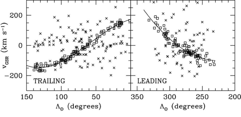
The trend of radial velocities along the trailing stream is well-defined (Majewski et al. 2004), enabling us to use kinematical information to prune Galactic interlopers and select a sample of extremely high-likelihood Sgr trailing arm stars. We draw such a sample from the Majewski et al. (2004) catalog, including all stars in the range for which radial velocity data has been obtained.444The sampling criteria of Majewski et al. (2004) required target stars to have infrared color , and be located within 5 kpc of the Sgr plane defined by Majewski et al. (2003). We fit a fourth-order polynomial to the radial velocity data as a function of orbital longitude, using an iterative rejection algorithm to produce our final clean sample of trailing arm stars (Figure 1, left panel).555We provide an online-only table of the coordinates and radial velocities in this clean sample at http://www.astro.virginia.edu/srm4n/Sgr. Note that we have not applied an explicit distance selection cut to the sample of stars plotted in Figure 1; if we were to do so it would remove a majority of the crosses from the left-hand panel as these stars lie significantly closer than the Sgr trailing arm stream (see, e.g., Figure 2 of Majewski et al. 2004).
The visible and well-defined portion of the trailing arm seen in the Southern Galactic Hemisphere 2MASS M giants is particularly important because it is dynamically young (torn off in the last 0-2 pericentric passages, depending on the assumed mass of Sgr) and has therefore experienced very little differential precession from the main body of Sgr (e.g., Helmi et al. 2004; Johnston et al. 2005). Observations (Majewski et al. 2003) indicate that the trailing debris stream is well-confined to a single plane, and numerical simulations show that -body debris in the range have angular momentum vectors aligned with that of the present satellite to within 1 degree for a wide range of models of the Galactic gravitational potential (see, e.g., Figures 4 and 5 of Johnston et al. 2005).
The lack of orbital precession in the trailing stream allows us to determine robustly the instantaneous angular momentum vector of Sgr. Using the sample of trailing arm stars defined above, we use a GC3 cell count technique (Johnston et al. 1996) to define the plane that best fits all of the trailing arm stars and the present position of the Sgr dwarf. For any given orbital pole the distance of star from the plane defined by the pole is
| (8) |
where is the orbital pole vector, is the vector from the Galactic Center to star , and is the vector from the Galactic Center to Sgr.
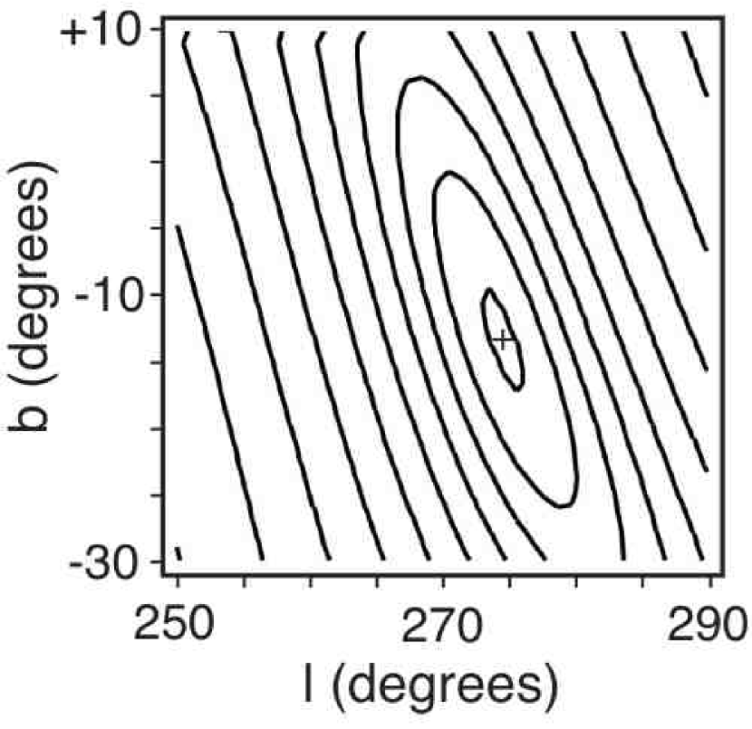
The best fitting plane is that which minimizes the sum over the 108 data points in the clean sample of trailing arm stars shown in Figure 1. In Figure 2 we plot as a function of , and demonstrate that the best-fitting orbital pole is . Unsurprisingly (since both the sample of stars and the technique were very similar), this is nearly identical to the trailing arm pole calculated by Johnston et al. (2005), although it differs slightly from the pole adopted by LJM05, who used the pole derived by Majewski et al. (2003) from fitting to both leading and trailing Sgr tidal debris.
3.3. Constraining the Orbital Speed of Sgr
Since the radial velocity vector and orbital pole (§3.2) of Sgr are known, the 3D space velocity of Sgr (, where by definition ) can be uniquely specified by the magnitude of the velocity of Sgr tangential to the line of sight:
| (9) |
In particular, for each choice of the Galactic halo parameters there is a value of that produces a trailing tidal stream whose velocities best match those shown in Figure 1. We converge upon this value in a manner similar to LJM05 by minimizing the statistic:
| (10) |
where is determined via linear interpolation of the model to the of each of the velocity data points .
There are two components governing the apparent velocity width of the stream; physical dispersion and observational uncertainty in the derived radial velocities. Majewski et al. (2004) find a net dispersion of 12 km s, composed of 6 km sintrinsic uncertainty in the velocity measurements and an underlying 10 km sphysical dispersion in the stream. For the purposes of Eqn. 10 it is irrelevant what the source of the dispersion is (since both will have identical effects governing the offset of stars from the orbital path) and we take km s. Rather than perform computationally intensive -body simulations to constrain for every choice of , we instead use test-particle orbits (see, e.g., LMJ09) to estimate the necessary value. Based on -body simulations with a wide range of Sgr masses and forms for the Galactic potential, we find a typical correction factor where the best-fit for -body models is systematically 4 km sslower than that implied by minimization using such test-particle orbits.

Considering the example case where and , in Figure 3 (bottom panel) we illustrate the dependence of on for three different values of . Note that there is a well-defined best value (which we call ) of for each ; we estimate the location of the minimum by fitting a simple third-order polynomial to as a function of . The resulting values of are well-behaved as a function of , as illustrated in the top panel of Figure 3.
For each choice of and it is possible to construct a similar relation. For the relation between and is practically unchanged (to within km s) for any choice of . For other choices of and the deviation of the relation from that shown in Figure 3 grows as departs from , but for the range of considered here these relations differ by less than 10 km s.
3.4. Constraining the Mass of Sgr
Data in the longitude range consist of a relatively orderly sample of trailing arm stars as they pass through the south Galactic cap moving predominantly transverse to our line of sight, and stars in this range can provide the most accurate measurement of the intrinsic velocity dispersion of the stream666There is a slight thickening in the distribution of radial velocities at because of the angular superposition of tidal debris from different epochs (i.e., stripped from Sgr on different pericentric passages) that occurs when this debris ‘piles up’ near the previous apogalactic point along the orbit.. Majewski et al. (2004) performed such an analysis, concluding that for a reasonable estimate of the observational uncertainty that the intrinsic velocity dispersion of the stream is km s. More recent, higher spectral resolution observations777Note that while we use the Monaco et al. (2007) velocity dispersion to derive the mass of Sgr, we used the Majewski et al. (2004) velocity dispersion in Equation 10 because this was the value appropriate to that more extensive sample of stars used to define the velocity trend of the trailing arm. by Monaco et al. (2007) have revised this value slightly to km s.
Since the velocity dispersion in the tidal debris streams reflects the mass present within the tidal radius of Sgr on the orbit immediately prior to that debris becoming unbound (see, e.g., Johnston et al. 1996; Johnston 1998; Peñarrubia et al. 2008), it can therefore be used to constrain the mass of the dSph (e.g., LJM05). We performed a series of 160 -body simulations in which satellites with 10 different initial masses ranging from were integrated along reasonable orbits for various lengths of time in different realizations of the Milky Way gravitational potential. The resulting relation between the final bound Sgr mass and the velocity dispersion is shown in Figure 4. Extrapolating from the best-fit polynomial to the curve, we conclude that a present bound mass produces the best fit to the observed velocity dispersion. Adopting a typical mass-loss history (generally similar along reasonable orbits in the range of Galactic potentials explored here), this implies that the original mass of Sgr was if it has been orbiting in the Galactic potential for Gyr. We adopt , corresponding to an initial Sgr scale length kpc (see Equation 7).

4. Constraining the Properties of the Milky Way Halo
We have now constrained the properties of Sgr itself as functions of the Galactic parameters . In the following subsections we go on to explore within which of these potentials the observational characteristics of the tidal streams are best reproduced.
4.1. Sgr Trailing Arm Properties
As defined in §3.3, we use the statistic to quantify the fit of a given -body simulation to the trailing arm velocity trend. While has already been minimized for a given choice of by determining the orbital velocity of the satellite, the precise minimum value can vary slightly between different halo realizations and we therefore also use it as a constraint on the properties of the Milky Way.
4.2. Sgr Leading Arm Properties
Although both the leading and trailing tidal tails are traced by the M-giant population, the location of Sgr slightly past pericenter along its orbit in combination with foreshortening of the orbital rosettes caused by our location 8 kpc from the center of the Milky Way means that while the trailing arm extends for across the southern Galactic hemisphere the leading arm is clearly visible only for (a significant section of which is obscured as it passes behind the Galactic disk/bulge). The exact track of leading Sgr debris as it passes through the north Galactic cap towards the anticenter is therefore uncertain in the 2MASS data since the M-giant tracer population is no longer as prominent in this older section of the stream. In contrast, SDSS imaging is sensitive to older Sgr populations, and clearly shows (Belokurov et al. 2006; Newberg et al. 2007; Cole et al. 2008) the Sgr leading arm arcing through the northern Galactic cap towards re-entry into the Galactic disk in the direction of the anticenter.
Belokurov et al. (2006) initially suggested that there may be a bifurcation in the angular position of the Sgr stream in the northern Galactic hemisphere, with a high surface brightness ‘A’ stream representing the primary wrap of the leading tidal arm passing through the coordinates and a lower surface-brightness ‘B’ stream representing a secondary wrap of the trailing tidal arm offset to higher declination around (see also Fellhauer et al. 2006). We adopt the positions of the ‘A’-stream survey fields of Belokurov et al. (2006) along this high-surface brightness branch as our constraint on the orbital path of leading Sgr tidal debris. These 17 pointings are tabulated in Table 1. Note that Belokurov et al. (2006) adopted a photometric distance scale calibrated against a distance to Sgr of 25 kpc. The distances listed in Table 1 have been rescaled to our adopted kpc by multiplying by a factor of 1.12.
We note that the dynamical origin of the lower surface-brightness B stream is uncertain: Recent observational data presented by Yanny et al. (2009) indicate that the A and B streams have indistinguishable trends in distance, radial velocity, metallicity, and mix of stellar types. This suggests that the A and B branches represent debris stripped from Sgr at similar times, and that the bifurcation may likely be within a single phase of tidal debris, originating in substructure within the initial Sgr dwarf (see discussion in §5.2). Since we do not attempt to constrain the internal structure of the Sgr dwarf (we focus here on exploring the effects of triaxiality in the gravitational potential of the Milky Way, and such an effort is beyond the scope of this contribution), we therefore do not explicitly constrain our model to match the B branch of the bifurcation.
Numerically, we define the statistic
| (11) |
describing the accuracy with which the declination of the -body model traces the A stream of Belokurov et al. (2006), and
| (12) |
describing the accuracy with which the angular width of the -body model matches the SDSS data at a right ascension (the non-spherical gravitational potential gives rise to angular broadening of the leading debris stream in this region due to differential precession). Based on the data presented by Belokurov et al. (2006), we estimate that the angular width of the stream as seen in SDSS is , with an uncertainty . In contrast to Equation 10 (which used as the variable coordinate), is determined via linear interpolation of the model to the right ascension of each of the SDSS survey fields along the main branch of the Sgr stream, each of which is assumed to have an angular uncertainty.888This is a rough estimate of the uncertainty in the centroid of the stream at a given right ascension based on the apparent width of the stream. .
While the trend of leading tidal debris is difficult to trace with 2MASS imaging data alone, the stream can be recovered using spectroscopy to identify the radial velocity signature of the stream. In Figure 1 we show our selection function for stars in the Sgr leading arm with (see §7.3) from the observational data presented by Law et al. (2004; see also LJM05), using a method similar to that adopted for trailing arm stars. This velocity trend has recently been confirmed by spectroscopic observation of a larger number of stars drawn from the SDSS imaging of the leading tidal stream (Yanny et al. 2009), in contrast with the preliminary conjecture by Newberg et al. (2007) that the velocity trend may be artificially produced by confusion in the leading arm M-giant sample. This gives our final constraint on the stream
| (13) |
where is determined via linear interpolation of the model to the orbital longitude of each of the observational data points in the 2MASS leading arm radial velocity sample. As for the trailing arm velocity constraint, we adopt an uncertainty km sfor each radial velocity measurement representing a combination of observational uncertainty and intrinsic stream width.
| RA | Dec | DistancebbDistances and uncertainties are taken from Belokurov et al. (2006) and scaled to reflect our choice of distance modulus to the Sgr core. |
|---|---|---|
| (degrees) | (degrees) | (kpc) |
| 215 | 4 | |
| 210 | 4 | |
| 205 | 4 | |
| 200 | 4 | |
| 195 | 7 | |
| 190 | 9.5 | |
| 185 | 11.2 | |
| 180 | 13 | |
| 175 | 13.75 | |
| 170 | 15 | |
| 165 | 16 | |
| 150 | 18.4 | |
| 145 | 19 | |
| 140 | 19.4 | |
| 135 | 19.5 | … |
| 130 | 19.5 | |
| 125 | 19.5 | … |
4.3. Combined Constraints
In general, the parameters are not separable and must be constrained simultaneously by , , , and . We combine these four constraints into a single statistic:
| (14) |
and seek the combination of that gives the global minimum for this combined statistic.
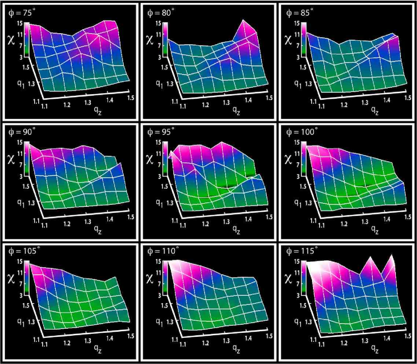
We performed a series of -body simulations covering the range , , with a grid spacing of in , 0.05 in , and 0.1 in . The resulting values of as a function of are shown in Figure 5 and demonstrate a general preference for values of in the range . Interpolating along the grid surface, the optimal fit () is achieved for , , . We use these parameters for our final best-fit -body simulation.
Since this optimal fit has there are obviously some residual imperfections in the model because different observational constraints favor different regions of parameter space. The greatest mismatch lies in the leading arm radial velocities (), followed by the leading arm angular coordinates (), the trailing arm radial velocities (), and lastly the angular width of the leading stream (). For comparison, the spherical halo model discussed by LJM05 is clearly a poor fit to the observational data (see Figure 10 of LJM05) and has . In general we deem simulations with to be visibly poor fits.
The optimal shape for the Galactic dark halo therefore appears to be an approximately oblate ellipsoid whose short axis is located in the Galactic disk along the direction . We note that this differs somewhat from that derived by LMJ09, who found a more strongly triaxial ellipsoid with , , by matching observed tidal debris to the orbital path of a point mass orbiting in the Galactic potential. It is well known, however, that actual leading/trailing arm debris falls inside/outside of the orbit respectively (e.g., Eyre & Binney 2009), meaning that a slightly different shape will be derived for the Galactic halo when attempting to match simulated debris to observed debris (as done in this contribution), rather than a simulated orbit to observed debris (as in LMJ09).
5. Model Overview
5.1. Model Summary
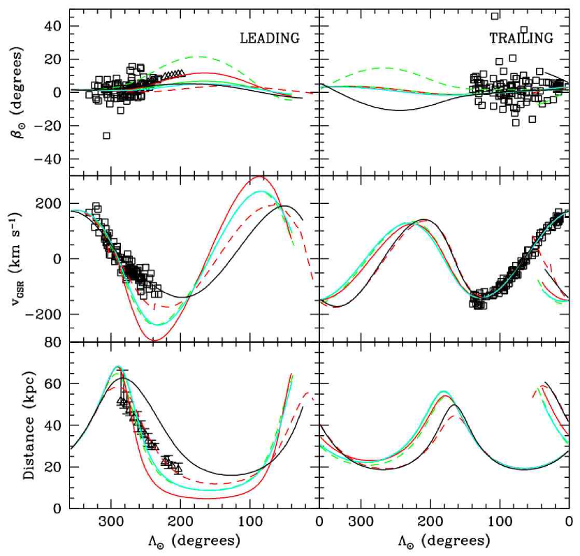
In LJM05, we presented possible models for the tidal disruption of Sgr under three different assumptions; that the Galactic halo was axisymmetric in the disk plane and either oblate, spherical, or prolate in the direction perpendicular to the disk. Neither of these three models were entirely satisfactory as they could not simultaneously reproduce the angular position, distance, and radial velocity trends of the leading arm. In contrast, our new model,999A complete data file for the dynamical and chemical characteristics of Sgr debris from this best-fit model is provided on the Web at http://www.astro.virginia.edu/srm4n/Sgr. orbiting in a non-axisymmetric dark matter halo, reproduces all of these constraints to reasonable accuracy as demonstrated by Figure 6. Indeed, we note that even though we didn’t explicitly fit to the distances of the SDSS leading arm data from Belokurov et al. (2006), the new model nonetheless matches them to within the uncertainty of the photometric calibration. While it is not possible to test the agreement of this new model with the distances of the M-giant sample directly (due to the evolution of the MDF along the Sgr tidal streams), we demonstrate in §7.3 that the model satisfactorily reproduces their apparent magnitude trend.
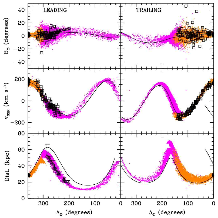
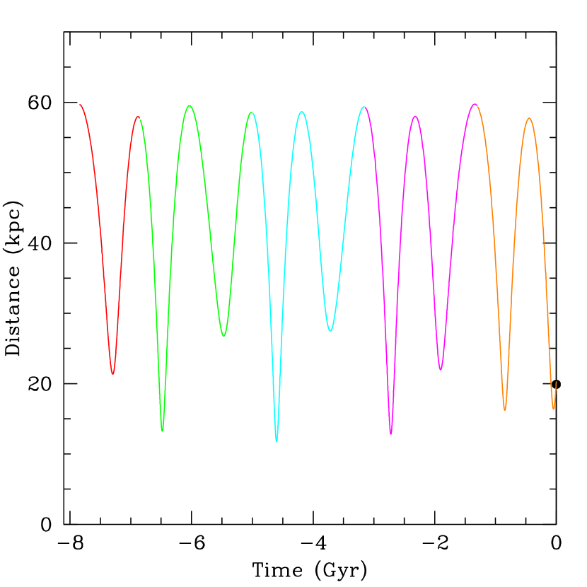
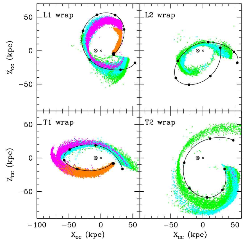
Since the Sgr streams frequently overlap themselves in all of the observable coordinates, it is useful to isolate specific wraps of the leading/trailing streams in order to discuss individual wraps more easily. By sorting the streams according to angular momentum (relative to the Sgr core) and time at which a given debris particle became unbound from the model satellite this is easily accomplished in the -body simulations. We color-code debris particles according to the time they became unbound from the satellite: Black points are currently bound to Sgr, orange points were stripped from the dwarf during the last two perigalactic passages (0 - 1.3 Gyr ago), magenta points during the previous two (1.3 - 3.2 Gyr ago), etc. (see Figure 7 for a detailed accounting of the color-coding scheme). As a convenient shorthand notation, we describe specific wraps of the streams as follows (see summary in Figure 8):
- L1:
-
Primary wrap of the leading arm of Sgr (i.e., angular separation from the dwarf). Traced by orange/magenta points near the Sgr dwarf, magenta/cyan/green points at larger angular separations.
- L2:
-
Secondary wrap of the leading arm of Sgr (i.e., angular separation from the dwarf). Traced almost entirely by cyan/green points.
- T1:
-
Primary wrap of the trailing arm of Sgr (i.e., angular separation from the dwarf). Traced by orange/magenta points near the Sgr dwarf, magenta/cyan/green points at larger angular separations.
- T2:
-
Secondary wrap of the trailing arm of Sgr (i.e., angular separation from the dwarf). Traced almost entirely by cyan/green points.
The major observational distinction of the present model from the oblate-halo model discussed by LJM05 is that the primary L1 wrap of the leading Sgr tidal stream is no longer predicted to pass closer than kpc to the Sun; the center of the L1 streamer intersects the Galactic disk at a distance of 13.5 kpc in the direction of the Galactic anticenter (see, e.g., Figures 6 and 8). This is consistent with the absence of net vertical flow observed in the solar neighborhood in recent radial velocities surveys (Seabroke et al. 2008).
Due to the triaxial Galactic potential, the orbital period and pericenter/apocenter of Sgr varies from orbit to orbit (Figure 7); the mean values of these parameters are 0.93 Gyr and 19/59 kpc respectively over the past 8 Gyr. The present space velocity of Sgr in this model is () = (230, -35, 195) km s. For our assumptions about the distance to Sgr, the Local Standard of Rest, and the solar peculiar motion this translates to a proper motion of mas yr-1 ( mas yr-1 in celestial coordinates) in the heliocentric rest frame. This agrees within with the proper motion measurements of Dinescu et al. (2005) who found mas yr-1 based on Southern Proper Motion Catalog values for 2MASS-selected giant star candidates, and within of the values mas yr-1 determined by Pryor et al. (2010). Our tangential velocity for Sgr ( km s) is also in good agreement with the measures of Irwin et al. (1996; km s) and Ibata et al. (2001b; km s). The mass of the Milky Way within 50 kpc in this model is (i.e., slightly smaller than that obtained by Sakamoto et al. 2003), corresponding to a halo scaling parameter km s(see Equation 3).
The present mass of the Sgr dwarf in this model is ; taking the apparent magnitude of the bound core of Sgr to be (Majewski et al. 2003) gives an absolute magnitude and luminosity for our adopted Sgr distance modulus (; Siegel et al. 2007) implying a mass/light ratio of . This is at the low end of the range estimated by LJM05; this difference reflects both our greater adopted distance to Sgr and our choice to use the higher-resolution Monaco et al. (2007) measurement of the dispersion of the Sgr stream instead of the previous Majewski et al. (2004) value. We note, however, that the derived mass is somewhat dependent on the structural model adopted for the Sgr dwarf. At present, the total interaction time of Sgr (and hence the initial mass of the satellite) is relatively unconstrained: With reasonable assumptions for its initial mass the length of the tidal streams observed in 2MASS and SDSS suggest that Sgr must have been disrupting for at least the last 3 Gyr (roughly corresponding to orange/magenta-colored points in Figure 6). We have opted to run our simulation for a significantly longer time ( Gyr) in order to make concrete predictions about where Sgr debris from earlier epochs may be expected; observational confirmation of the presence or absence of such older debris streams will provide a strong constraint on the actual length of the interaction time. Future models that more accurately treat the dark/light matter separation and are constrained to reproduce the bar-like core structure of Sgr (e.g., Łokas et al. in prep.) may provide more stringent constraints on the ratio of the dwarf.
5.2. The Nature of the Bifurcation
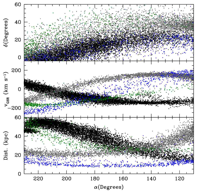
As indicated by Figure 6, our simulations match the high surface-brightness (hereafter HSB) track of the leading arm in the ‘Field of Streams’ region described by Belokurov et al. (2006) but do not produce a bifurcation in the form of a low surface-brightness (hereafter LSB) branch offset to higher declination. Fellhauer et al. (2006) previously explained this bifurcation as the juxtaposition of the young ( Gyr) L1 wrap of the leading arm with the old ( Gyr) T2 wrap of the trailing arm.101010Note that Fellhauer et al. (2006) call the equivalent of their L1/L2/T1/T2 streams the A/C/D/B streams respectively. This explanation is not viable for the current model: As illustrated in Figure 9, the distance/radial velocity trends of the L1 (black points) and T2 (green points) streams are markedly different, in contrast to Yanny et al. (2009) who demonstrate that the distance and radial velocity trends of the LSB and HSB streams are indistinguishable.
However, we note that the Yanny et al. (2009) observations are not reproduced well by the Fellhauer et al. (2006) model either: This model predicts a factor difference in distance between the LSB and HSB streams at that is not observed. Additionally, given the strong evolution in the MDF with increasing separation from the Sgr dwarf (e.g., Chou et al. 2007) we should not expect the metallicity of the LSB and HSB streams to be similar (as observed by Yanny et al. 2009) if they represent extremely different dynamical ages of tidal debris. Certainly, if the LSB stream were significantly older than the HSB we should not expect the LSB stream to contain as many M-giants as the HSB stream since M-giants are a young tracer population.
-body models of Sgr tidal destruction also predict that the young T1 trailing arm should pass through the Field of Streams region. In both the model presented here and the model described by Fellhauer et al. (2006), the T1 wrap traverses this region from to with a distance varying from kpc to kpc, and radial velocity varying from km sto km s. Such tidal debris (grey points in Figure 9) is not observed in the Field of Streams, suggesting that the Sgr tidal streams are insufficiently long to produce T1 trailing tidal debris in this region of sky (or at least, that the stellar density in the stream is declining sufficiently rapidly that it has not been detected in the SDSS). This places a limit on the length of the Sgr tidal stream similar to that derived from other observational constraints that the Sgr tails represent Gyr worth of tidal debris. If the Sgr tails are so young, we should not expect any debris corresponding to earlier wraps (i.e., T2/L2) to exist and it is correspondingly impossible to interpret the bifurcation as the juxtaposition of Sgr tidal debris torn from Sgr at significantly different times.
We therefore favor the explanation proffered by Yanny et al. (2009) that both the LSB and HSB streams may represent debris stripped from Sgr at similar times. Indeed, we note that models of Sgr orbiting in a non-spherical Galactic potential exhibit precessional broadening of the angular width of the leading debris stream in this region which manifests as a low surface brightness ‘spray’ to higher declinations similar to that of the LSB stream (this effect is increasingly noticeable for haloes with stronger departures from spherical symmetry). This presents an alternative scenario wherein the bifurcation may arise due to substructure within the initial Sgr dwarf, such as a smaller dwarf satellite that may have been bound to Sgr when it fell into the gravitational potential of the Milky Way (see, e.g., Chou et al. 2009; Law et al. in prep), or simply to anisotropy of the stellar orbits within the original dwarf which might be expected to give rise to tidal debris occupying only a subset of the angular width covered by our isotropic -body model.
The detailed nature of the low surface brightness branch in the SDSS view of the Sgr stream is therefore unknown at present, and is not possible to reconcile with -body models that fit the unambiguous primary leading and trailing tidal streams illustrated in Figure 6. While this feature may ultimately provide a constraint on the internal structure of the initial dSph satellite, exploration of such structure is beyond the scope of this contribution.
6. Discussion: The Shape and Orientation of the Milky Way Dark Matter Halo
Cold dark matter (CDM) models of galaxy formation generally predict that dark haloes should be mildly triaxial (e.g., Bullock 2002; Jing & Suto 2002; Bailin & Steinmetz 2005; Allgood et al. 2006; and references therein), predominantly prolate systems (; Allgood et al. 2006) with characteristic central axis ratios111111We adopt a convention in which axial ratios such as are given with a subscript of () to indicate that they are measured with respect to the potential (density) contours. , (Hayashi et al. 2007). While there is a tendency for haloes to be more spherical at larger radii (Allgood et al. 2006; Hayashi et al. 2007), the halo of Milky Way-like systems at a distance of kpc is expected to be prolate with (based on the Via Lactea simulation of Diemand et al. 2007; Kuhlen et al. 2007).
Observationally, typical haloes appear to be rounder than predicted by collisionless CDM simulations, as indicated by gravitational lensing mass models (e.g., Hoekstra et al. 2004; Mandelbaum et al. 2006; Evans & Bridle 2009), polar ring galaxies (e.g., Iodice et al. 2003), and X-ray isophotal studies (e.g., Buote et al. 2002; although c.f. Diehl & Statler 2007; Flores et al. 2007). This possible mismatch is perhaps unsurprising because the growth of baryonic structures within these haloes tends to make them considerably rounder (e.g., Debattista et al. 2008; Valluri et al. 2009), inflating the principal axis ratios by as much as within the virial radius (Kazantzidis et al. 2004). However, it is difficult to constrain the actual triaxiality of individual haloes because galaxies are projected onto the two-dimensional plane of the sky and observations are relatively insensitive to the mass distribution along the line of sight (although c.f. Corless et al. 2009).
It is therefore noteworthy that for the only galaxy where we have a fully three-dimensional view from the interior of the mass distribution (i.e., the Milky Way) it appears (§4.3) that the best-fitting axial ratio at radii kpc describes an almost perfectly oblate ellipsoid with minor/major axis ratio , intermediate/major axis ratio , triaxiality , and the minor axis located in the plane of the Galactic disk in the direction . In this section we discuss the physical interpretation of these results, along with possible effects that could influence our derivation of the halo shape.
6.1. Physical Validity of the Triaxial Halo Model
6.1.1 Tracing the Underlying Mass Distribution
In §2.1 we introduced flattening directly into the contours of the gravitational potential because this was analytically tractable and consistent with the method of previous studies (in particular LJM05). It is well-known however that as the ellipticity of the potential becomes more extreme, the corresponding mass distribution required to generate it may become unphysical (i.e., have regions of negative mass). In order for any model of the Galactic halo to be believed, it must correspond to a physically realizable density distribution.
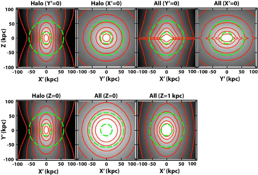
In Figure 10 we show the corresponding contours of the mass distribution underlying our best-fit model for the Milky Way (as calculated by taking the Laplacian of the gravitational potential). As expected, the mass distribution is less spherical than the isopotential surface; the contours of the dark matter halo are approximately elliptical at small radii (i.e., within kpc) with , , and . Although some pinching of the dark matter density contours is apparent at larger radii the mass distribution is everywhere positive. Figure 10 also demonstrates that while addition of the baryonic mass component significantly changes the net density distribution at small radii and near the Galactic disk plane, the density distribution at larger radii probed by the orbit of Sgr is dominated by the dark halo component.
We additionally confirmed the validity of our results by constructing a triaxial NFW (Navarro et al. 1996) halo model in which the axial flattenings were introduced in a more physically motivated manner directly into the mass distribution and where the resulting accelerations were computed using the approximate form of the corresponding potential given by Lee & Suto (2003). As expected, there are slight differences in the path of satellites orbiting in this NFW halo and in our best-fit logarithmic potential, but these differences are minor and likely due to the fact that we did not fine tune the NFW model.
6.1.2 Orientation of Principal Axes
While the mass distribution underlying our best-fit model of the Galactic halo is physically reasonable, the orientation of the halo (i.e., strongly non-axisymmetric in the plane of the Galactic disk, with the angular momentum vector of the disk aligned with the intermediate axis of the halo) is unexpected because orbits about intermediate axes tend to be unstable (e.g., Adams et al. 2007). This is not a concern for stellar orbits in the Galactic disk because the gravitational potential at small radii kpc is dominated by the (nearly) axisymmetric baryonic mass distribution rather than the triaxial dark halo. Indeed, preliminary results of orbit integration in the gravitational potential derived here indicate that loop orbits are permitted, suggesting that a self-consistent disk may still be supported (R. Johnson and K.V. Johnston, private communication, 2010). However, this situation begs the question of why the Galactic disk formed in its present orientation unless the principal axes of the dark halo either twist substantially with radius (in contrast to the general prediction of Hayashi et al. 2007) or evolve with time. While we cannot rule out the possibility that rotation of the dark halo has contributed in some regard to our results, we neglect such effects because typical haloes are expected to rotate extremely slowly (e.g., Bullock et al. 2001a; Herbert-Fort et al. 2007, 2008; Bett et al. 2009).
Typically, simulations of disk galaxy formation suggest (e.g., Debattista et al. 2008) that the minor axes of the dark halo and the baryonic disk should be approximately aligned (to within an average of ; see discussion by Warren et al. 1992; van den Bosch 2002; Bett et al. 2009) because both are formed from accreted matter with similar specific angular momenta. If a disk were to form in an elliptical halo potential such as that proposed in §4.3, simulations suggest that the disk too should become elongated and non-axisymmetric (see, e.g., Gerhard & Vietri 1986; Debattista et al. 2008). It will therefore be intriguing to investigate whether the relative orientation of the host dark matter halo and baryonic disk proposed here can be strongly motivated within the current CDM paradigm.
It is worth asking as well whether such an inclined oblate halo can explain the observed distribution of Galactic satellites, which simulations suggest (Zentner et al. 2005) should be distributed along the major axis of the host halo (i.e., have a pole aligned with the minor axis). The Fornax-Leo-Sculptor great circle has a pole (Lynden-Bell 1982; see also Kunkel & Demers 1976; Majewski 1994; Fusi Pecci et al. 1995), and a recent update (Metz et al. 2007, 2009) including the faint new dwarfs discovered in the SDSS gives a revised satellite pole . The updated pole of Metz et al. (2009) lies within of the minor axis we derive for the Galactic halo, but it is difficult to determine whether this similarity is simply an unrelated coincidence.121212If the probability distribution of the satellite pole were uniform across the entire sky, the chance for it to be coincidentally aligned with to within is %.
6.2. Alternatives to the Triaxial Halo Model
In LJM05, we conducted an extensive parameter space search in an effort to find a combination of Milky Way + Sgr parameters capable of simultaneously matching both the observed angular position and distance/radial velocity trends of leading tidal debris. In particular, we explored the effect of varying the proper motion of Sgr (), the distance to Sgr (), the distance from the Sun to the Galactic Center (), the total mass of the Galactic disk (via the scaling parameter in Equation 1), the dark halo scale length (), the dark halo flattening perpendicular to the disk (), and the total mass scale of the Milky Way as parameterized by the rotation speed of the Local Standard of Rest ().
Although the Galactic disk contributes significantly to the overall flattening of our adopted Galactic potential at small radii (e.g., Figure 10), it has only a minor effect at the range of radii ( kpc) probed by the orbit of Sgr. As demonstrated by Figure 11, the dark halo in our model is the dominant contributor to the total gravitational potential at these radii. Indeed, if we decrease the mass of the Galactic disk by 50% (by setting in Equation 1) and increase the total halo mass correspondingly (so that the Local Standard of Rest remains constant at km s), we can repeat the parameter space search described in §4. Scaling the proper motion of Sgr to again best-fit the trailing-arm velocity trend, we find optimal values for almost identical to those derived previously (although the overall of the best-fit model is not as good as for the case ). We are therefore confident that the details of the Galactic disk model do not significantly bias our results.


Similarly, the details of the triaxial Galactic bar (which we did not include in our model) and stellar halo are unlikely to change our results. Neither are sufficiently massive to have a great effect on the gravitational potential at distances kpc, and neither have orientations akin to that which we derive for the dark halo. The major axis of the bar is thought to lie within of the -axis (e.g., Blitz & Spergel 1991; Nakada et al. 1991; Morris & Serabyn 1996; Babusiaux & Gilmore 2005), similar to the minor axis of the dark halo. While the stellar halo is significantly triaxial (, , ; Newberg & Yanny 2006; see also Larsen & Humphreys 1996; Xu et al. 2006) with a major axis lying approximately in the Galactic plane ( from the axis) the minor axis is not apparently contained within the plane but located from the axis.
Throughout the entirety of the LJM05 parameter space search, the only parameter that was found to have a significant effect on the angular position/distance/radial velocity trend of the Sgr leading arm was the flattening of the dark halo . Although no single choice of can simultaneously reproduce all observational constraints, we have demonstrated (see also LJM09) that a fully triaxial model in which the short axis is approximately aligned with the Galactic axis is capable of doing so.
Such a triaxial halo is therefore obviously attractive in the sense that only -body models in such a halo succeed in modeling the Sgr – Milky Way system where previous efforts (e.g., Helmi et al. 2004; LJM05; Fellhauer et al. 2006; Martínez-Delgado et al. 2007) have failed. Despite the extensive exploration of parameter space undertaken by ourselves (this paper; LJM05; LMJ09) and other groups (e.g., Helmi et al. 2004; Fellhauer et al. 2006; Martínez-Delgado et al. 2007) however, the space explored to date is far from exhaustive and it is possible that the triaxial halo model may prove to be simply a numerical crutch that mimics the effect of some as-yet unidentified alternative. In the following sections, we briefly discuss a few possibilities that may obviate the need for triaxiality to explain the extant data.
6.2.1 Alternative Formulations for the Gravitational Potential
While we have focused on a logarithmic formulation of the Galactic gravitational potential, other forms could also reasonably be adopted. In LJM05 we explored axisymmetric NFW (Navarro et al. 1996) models and were unable to resolve the halo conundrum. As demonstrated in §6.1.1 however, fully triaxial NFW models can give rise to orbits for Sgr that match the observed angular precession and distance/radial velocity trends of leading tidal debris. We find that orbits within logarithmic and NFW haloes are sufficiently similar that there is no reason to differentiate between the two for our present purposes.
Fellhauer et al. (2006) claim that a mass distribution of the form specified by Dehnen & Binney (1998) can produce some effects similar to prolateness in a logarithmic halo. However, using such a model these authors were nevertheless unable to reproduce the distance trend of leading tidal debris as seen in the SDSS (Belokurov et al. 2006) and concluded that their Set D of proper motions for Sgr (i.e., those derived by LJM05) in a logarithmic halo provided the best overall fit to the observational data then available. We therefore find no reason to prefer a Dehnen & Binney (1998) model over the triaxial logarithmic halo model presented here.
6.2.2 Evolution in the Orbit
Although our model dSph has been orbiting in the Galactic potential for 8 Gyr, we have not considered the influence of any evolution in either the orbit of Sgr or the underlying gravitational potential of the Milky Way. We expect there was actually evolution in both the depth, and the shape of the potential (e.g., Kuhlen et al. 2007). While we expect the streams to be independent of past evolution in the potential of the Milky Way (since tidal streams respond adiabatically to changes in their host potential; see discussion by Peñarrubia et al. 2006) some evolution has certainly occurred in the orbit of Sgr since it fell into the Milky Way. Dynamical friction and other such evolutionary effects therefore reflect an uncertainty in our models, although we note that (as discussed by LJM05) such effects alone are unlikely to be able to resolve the halo conundrum. Further investigation of these effects must (among other things) properly account for the relative distribution and mass-loss history of both the dark and baryonic matter in Sgr, and is therefore beyond the scope of this contribution.
6.2.3 Dwarf — Tail Gravitational Interaction
As discussed by Choi et al. (2007), the gravitational influence of the bound satellite on debris in the tidal tails can shift the trajectories of actual tidal debris away from the orbital path traced by the bound core of the dSph. For sufficiently massive satellites (greater than % the virial mass of the host), this effect can be appreciable and degenerate with that caused by flattening (or triaxiality) in the underlying gravitational potential of the Milky Way. However, we note that despite claims to the contrary (Choi et al. 2007) our simulations fully account for this effect; the self-gravity of the bound satellite is applied to all -body particles at all times regardless of whether or not they are in the Sgr core or in the tidal tails.
6.2.4 Gravitational Influence of the Magellanic Clouds
The Large Magellanic Cloud (LMC) is kpc distant in the direction ) (van der Marel et al. 2002), placing it within kpc of the Galactic plane. Based on great-circle fits to the Magellanic stream, the pole of the system appears to be ) (Nidever et al. 2008). That is, the pole of the Magellanic stream is aligned with the short axis of the Galactic dark halo as derived in this contribution to within in Galactic longitude.131313They differ by in Galactic latitude, but the symmetry axes of the dark halo were fixed to lie at . This suggests two possibilities: (1) The Magellanic Clouds may have fallen into the Milky Way along the plane of the long and intermediate axes of the dark matter halo (i.e., the alignment is a consequence of the dark matter distribution), or (2) the Magellanic Clouds may exert a significant gravitational acceleration on the Sgr dwarf, with the mass of the Clouds at large radii in the plane mimicking the effect of an extended dark matter distribution in this plane (i.e., the alignment is the cause of the apparent dark matter distribution).
A precise description of the second scenario would require a comprehensive model for the orbital and mass-loss history of the Magellanic Clouds, but it is possible to understand the magnitude of their gravitational influence on the path of Sgr tidal debris by integrating massless test-particles along the Sgr orbit in a Milky Way with a spherical dark halo and simplified model of the LMC. We first test the effect of introducing a fixed point-mass into the gravitational potential of the Milky Way at the present location of the LMC, whose mass is allowed to vary from - 10% of the total mass of the Milky Way within 50 kpc (i.e., ). As illustrated in Figure 12, a fixed LMC with a mass 10% that of the Milky Way can produce a significant deviation on the order of in the orbital path of leading Sgr tidal debris.
Of course the LMC is not fixed in space, but describes an orbit about the Milky Way confined approximately to the plane. We therefore develop a second, slightly more realistic model in which the LMC is described in a time-integrated sense by a ring of mass at a radius of 50 kpc in the plane. The gravitational acceleration at an arbitrary point in space resulting from such a configuration is described using an analytical approximation to the numerically evaluated elliptical integrals (see derivation for the electrostatic case by Zypman 2005). This second model produces even more noticeable deviations from the original orbital path, with appreciable shifts in both the leading arm angular position and radial velocities expected for models in the range of masses % that of the Milky Way.
The detailed effect of the Magellanic Clouds on the orbit of Sgr is extremely uncertain. Both our point-mass and ring-mass models are obviously oversimplifications, neglect the SMC entirely, and assume that the gravitational influence of the LMC has been fixed over the entire interaction history of the Sgr dwarf ( Gyr in the current model). Since the Clouds are currently thought to be near the pericenter of their orbit, for the majority of the lifetime of Sgr they likely lay at greater distances where their gravitational force would be smaller. Indeed, some recent lines of investigation suggest that they may have only recently fallen into the gravitational potential of the Milky Way for the first time (e.g., Besla et al. 2007), drastically limiting the time during which they could have torqued the orbit of the Sgr dwarf. Of the various orbital paths shown in Figure 12, only the triaxial halo model actually succeeds in reproducing all of the observational data. However, given the myriad uncertainties in the Milky Way - LMC - Sgr system the important conclusion to draw is that gravitational peturbations from the Magellanic Clouds may be sufficient to torque the leading arm of the Sgr stream significantly, especially if the effect is enhanced by the response of the Milky Way dark matter halo itself to the passage of the Clouds (see, e.g., Weinberg 1998).
6.2.5 Alternative gravity
Modified Newtonian gravity (MOND; see Milgrom 1983; Bekenstein 2004) on Galactic scales has been proposed as an alternative theory to explain the flat rotation curves typical of galaxies without recourse to an extended halo of dark matter. Read & Moore (2005) demonstrated that MOND was an equally viable alternative to the oblate dark matter halo model presented by LJM05, capable of fitting the angular position of the leading tidal debris but not the radial velocities. Now that a dark matter model has been able to successfully match both observational constraints, it is worthwhile to investigate whether a similarly successful MOND model can be constructed. Since the key to resolving the halo conundrum appears to have been the inclusion of a strongly non-axisymmetric component to the gravitational potential, it is not immediately obvious how such a potential could be produced in a MOND model by the predominantly axisymmetric distribution of baryonic matter typically adopted for the Milky Way (although c.f. Wu et al. 2008; Widrow 2008).
6.3. Testing the Model
Fortunately, the model presented here for the shape, size, and orientation of the Galactic gravitational potential is easily testable; it must be capable of explaining the orbital paths of other Galactic satellites that similarly provide constraints on the mass distribution in the Milky Way. Typically, previous studies of tidal debris systems in the Galactic halo have only explored the effects of changing the axial scalelength perpendicular to the Galactic disk (i.e., ), and it is unclear whether satisfactory solutions for other satellites can be found in such a strongly non-axisymmetric potential as that suggested here. In particular, can realistic orbits be found to match such systems as the Monoceros tidal stream (e.g., Peñarrubia et al. 2005), the Magellanic Clouds141414While simulations generally favor haloes which are extended along the Galactic axis (similar to those in the triaxial model), preliminary results indicate that the Magellanic Clouds are relatively insensitive to the distribution of mass along the Galactic axis and can neither confirm nor deny the triaxial model presented here (G. Besla, priv. comm.). (e.g., Besla et al. 2007; Rŭžička et al. 2007), the “orphan stream” (Belokurov et al. 2007), the GD-1 stream (Koposov et al. 2009), the newfound Cetus Polar Stream (Newberg et al. 2009), and tidally disrupting Galactic globular clusters such as Pal 5 (Odenkirchen et al. 2009)? Similarly, is a triaxial Galactic halo consistent with observations of the Galactic HI disk (e.g., Olling & Merrifield 2000; Kalberla et al. 2005; and references therein)? It is intriguing that Saha et al. (2009) discuss evidence to suggest that the dark matter halo must be similarly non-axisymmetric in the Galactic plane in order to explain the asymmetric flaring of the disk (although c.f. Narayan et al. 2005). Future observations of hypervelocity stars at large distances may also provide key diagnostics (e.g., Gnedin et al. 2005; Yu & Madau 2007; Perets et al. 2009).
7. Explaining the Evolution of the MDF along the Tidal Streams
Recently, numerous measurements have been made (e.g., Vivas et al. 2005; Chou et al. 2007, 2009; Monaco et al. 2007; Yanny et al. 2009; Starkenburg et al. 2009) of the metallicity distribution function (MDF) along the Sgr stream, although a uniform picture of the evolution of the MDF is difficult to construct because systematic differences in the metallicity sensitivity between stellar populations traced by various surveys can bias the resulting trends. However, significant evidence is starting to emerge for a gradient of the MDF with Sgr orbital longitude. Bellazini et al. (2006) for instance observed that the ratio of blue horizontal branch to red clump stars changes between the main body of Sgr and the stellar streams (demonstrating an age/metallicity gradient), and similar claims of such evolution have been made by Monaco et al. (2007) who found that while the core of Sgr has a mean metallicity the tidal streams have a mean metallicity of . The most comprehensive picture presented to date however has been that of Chou et al. (2007), whose uniform selection technique demonstrates that the MDF of the Sgr M-giant population continuously evolves from a median in the Sgr core to dex over the length of the leading tidal arm.
In this section, we attempt to reproduce the gradient in the MDF by making physically motivated assumptions about the star formation history of the Sgr dwarf. We consider only the M-giant population observed by Chou et al. (2007) and Monaco et al. (2007) in order to ensure a uniform selection function at all orbital longitudes. While Chou et al. (2009) have recently extended their earlier work (Chou et al. 2007) by additionally measuring the evolution in the abundance patterns of titanium (Ti), yttrium (Y), and lanthanum (La), we do not incorporate these additional elements into our analysis.
7.1. Enrichment Model
Generally, we expect that star formation in Sgr is likely to have occurred near the bottom of its gravitational potential well, and that stars thus formed in the core would gradually diffuse outwards with time. Remnants of such stellar populations would tend to persist in the Sgr core until the present day and we therefore assume that the stellar populations present in the Sgr streams correspond to counterparts in the Sgr core. These Sgr core populations have been traced using high-precision HST-ACS photometry by Siegel et al. (2007), who find five major star formation episodes:
- Population A:
-
M54 metal-poor population.
, age Gyr. - Population B:
-
Sgr metal-poor population.
, age Gyr. - Population C:
-
Sgr intermediate population.
Three sub-populations:
C1: , age Gyr,
C2: , age Gyr,
C3: , age Gyr. - Population D:
-
Sgr young population.
, age Gyr. - Population E:
-
Sgr very young population.
, age Gyr.
Younger stellar populations might be realistically assumed to be more tightly bound than older populations, which have had more time to diffuse outward in the dwarf. Motivated by the presence of such population gradients within other Galactic dSphs (e.g., Tolstoy et al. 2004) for which the more metal-rich populations are more centrally concentrated and have lower velocity dispersion, we tag particles in our best-fit model of the Sgr dwarf to correspond to different stellar populations according to their total energy in the pre-interaction dSph. The energy of an individual particle in the satellite is given by
| (15) |
where is the velocity and the internal potential energy of particle relative to the satellite. For convenience, we define to be an order-sorted version of the energy distribution, ranging from 0 (most strongly bound particle) to 1 (least bound particle) with a uniform distribution in the range .
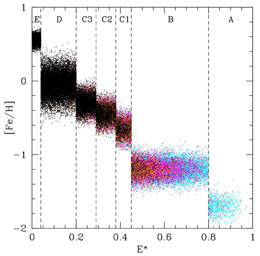
We assign particles with a given range of to each population as illustrated in Figure 13, the locations of the energy divisions (and hence the total number of particles assigned to each burst of star formation) are free parameters. Once a particle has been assigned to a given population, we assign it a metallicity and age based on a Gaussian random selection about the mean and standard deviation of the population given in the list above, and randomly choose an infrared color uniformly from the range . Adopting Marigo et al. (2008) isochrones151515We use the interface made available by L. Girardi at http://stev.oapd.inaf.it/cgi-bin/cmd with a Chabrier (2001) IMF for each of the simulated populations, we calculate the absolute magnitude for each simulated particle, adopting a 50%/50% mix of RGB and AGB stars. This particular mix of RGB/AGB stars is not intended to match any particular distribution, but to illustrate the general range of magnitudes expected for stars in each evolutionary phase. We note that not all of the Siegel et al. (2007) populations will produce M-giants: Population A in particular is too old and metal-poor.161616Indeed (as discussed by Siegel et al. 2007), the M54 metal-poor population may have formed separately from Sgr and later been accreted by the dwarf, since M54 has a distinct stellar population and radial profile and Sgr is nucleated even ignoring this population (e.g., Monaco et al. 2005). All this means, however, is that we would not expect regions of the stellar streams populated by these stars to be traced by M-giants of those metallicities, and we therefore do not calculate magnitudes for these particles.
Strictly speaking, the enrichment model presented here is unphysical since it assumes that all of the stellar populations were present in Sgr at all times during its Gyr interaction history with the Milky Way, despite the fact that some of these populations didn’t form until many Gyr later. This is an inescapable consequence of the -body method adopted in this paper — particles cannot readily be introduced into the simulation at arbitrary times. Ideally, a fully hydrodynamical simulation could build a gas-phase component into the model dwarf, and permit this to form stars at the appropriate times. How to retain an appreciable gas supply in Sgr until only a Gyr ago is a challenging question in its own right, but claims of a detection of gas removed from Sgr as recently as Gyr ago by its most recent passage through the extended Galactic disk have been made by Putman et al. (2002). Since the -body particles only represent dynamical tracers however, we content ourselves with noting that no appreciable quantities of any given stellar population are tidally stripped from the dwarf in this model before they are thought to have formed (see horizontal dashed lines in Figure 14).
7.2. Matching the Observed MDF
Tidal stripping of a satellite on an eccentric orbit such as that of Sgr occurs nearly impulsively, with the majority of tidal debris stripped in the brief time interval that the satellite is passing through the pericenter of its orbit. Although the overall trend with successive pericentric passages is to remove stars at successively smaller radii or energies (i.e., ‘onion-skin’ style stripping models, see discussion by Martínez-Delgado et al. 2004), each mass loss event does not impose a sharp tidal cutoff on the stellar populations of the dwarf. Rather, the rapidly changing tidal radius, the impulsive nature of the stripping, and the dependence of the effectiveness of tidal stripping on the orientation of individual stellar orbits (see, e.g., Read et al. 2006a) means that on any given pericentric passage Galactic tides reach deeply into the satellite and can unbind stars from a variety of populations. This does not completely evacuate the energy/radius range of particles in the satellite, and the remaining stars rapidly relax back to a Plummer model over a dynamical time ( Gyr; see, e.g., discussion by Peñarrubia et al. 2008, 2009). Despite the sharp divisions that we introduced in the distribution of stellar populations within the model satellite, there is significant overlap in the populations expelled from the satellite into the tidal tails over the lifetime of the dwarf. This is illustrated in Figure 14: While particles assigned to Population A are almost entirely stripped from the dwarf during the first two to three orbital periods, stars in Population B are present in many successive epochs of tidal debris and still have a residual bound population (black points at ) in the dwarf at the present day. Stars in Population D are present in only the most recent tidal debris. The trend of stellar populations along the tidal streams is further affected by the angular phase smearing caused by the differential orbital velocities of stripped stars from each epoch of tidal debris.

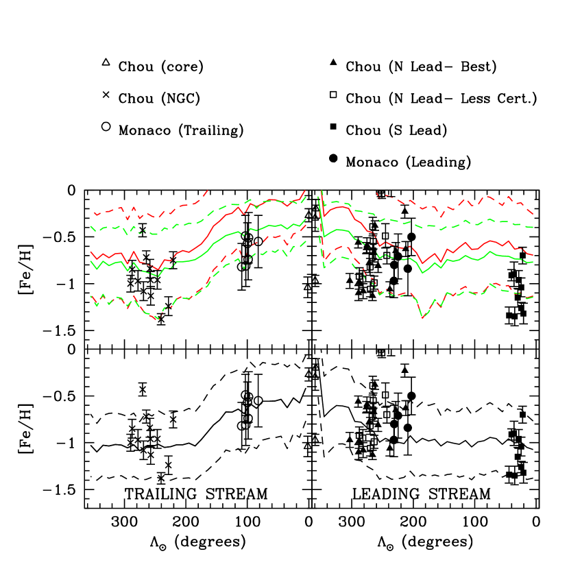
By adjusting the relative sizes of each of the stellar populations (i.e., sliding the vertical lines in Figures 13 and 14) it is possible to adjust the relative balance of stars of a given metallicity present in each debris era (i.e., point ‘color’), and thereby as a function of orbital longitude along the Sgr tidal streams. In Figure 15 we plot the metallicity of stars observed by Chou et al. (2007) and Monaco et al. (2007; their SARG subsample) as a function of orbital longitude, overplotted with the mean metallicity of the simulated Sgr stream using three different assumptions about the energy ranges assigned to each of the Populations A-E. The simplest possible assignment in which Populations A/B/C/D/E correspond to uniformly wide energy ranges respectively fails to match the observational data. As illustrated by the red curves in Figure 15, the highest-metallicity debris is over-represented in the regions of the stream nearest the satellite (i.e., and in the leading/trailing streams respectively), and Population C is over-represented relative to Populations A and B at larger angular separations (i.e., the model stream is too metal-rich at and in the leading/trailing streams respectively). It is possible to suppress the presence of the youngest stellar populations in the Sgr stream by reducing the range in assigned to them, and the green curves in Figure 15 show the result of adopting energy ranges for Populations A-E respectively. While this improves the agreement in the regions of the tidal tails nearest Sgr, the mean model metallicity is still too high at larger angular separations.
We find that a reasonable fit to both the low- and high-angular separation observational data is achieved with a choice of energy ranges for Populations A/B/C1/C2/C3/D/E respectively (black lines in Figure 15). Given the large spread of the observational measurements and the large number of assumptions made by our debris-tagging method, a more precise determination of the best-fit choice of energy ranges is not warranted. Rather, we conclude that for some choice of the energy ranges it is possible to broadly fit the observational trends: The mean metallicity of the model Sgr stream decreases from [Fe/H] in the core to [Fe/H] at large angular separations.
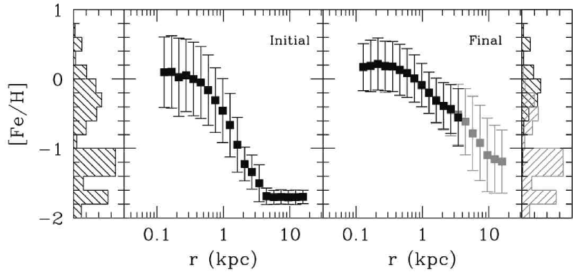
The above choice of energy ranges corresponds to a reasonably strong dex metallicity gradient with radius in the initial model Sgr dSph (Figure 16, left-hand panel), consistent with the prediction of Chou et al. (2007), and slightly stronger than observed in the Sculptor dSph by Tolstoy et al. (2004). The strong initial gradient is largely erased by the process of tidal stripping, leaving a relatively weak metallicity gradient dex remaining by the present-day (Figure 16, right-hand panel). The MDF of the bound core of the model Sgr dwarf (Figure 16, right-inset black histogram) is therefore significantly different than both the MDF of the original dSph (Figure 16, left-inset black histogram) and the MDF of the stellar tidal debris that Sgr has contributed to the Galactic halo (Figure 16, right-inset grey histogram). If such strong tidal evolution of the MDF is common for Galactic satellites, it may partially explain the observed chemical abundance mismatch between Galactic halo stars and the present-day dSph population (e.g., Geisler et al. 2005; and references therein). Rather than requiring the early accretion onto the Milky Way of metal-poor, high [/Fe] satellites that are completely disrupted by the present day (e.g., Font et al. 2006), the metal-poor halo stars may simply have originated in the dSphs with which we are familiar, and in which few traces of the originally sizeable metal-poor populations now remain (e.g., Majewski et al. 2002; Muñoz et al. 2006; Chou et al. 2009).
7.3. K magnitudes of M giants
One of the challenges in attempting to trace Sgr debris in the 2MASS M-giant view originally provided by Majewski et al. (2003) was that as the metallicity of stars evolves along the stream, so does the zeropoint of the photometric distance calibration. Since the distance calibration was tied to the relatively metal-rich Sgr core, distances become systematically more inaccurate with increasing separation from the core. Now that we have a model for the evolution of metallicity along the streams, we can perform the comparison of simulations and observational data in a purely observational apparent magnitude space.
In Figure 17 we plot the apparent magnitude, angular position , and radial velocity for the simulated Sgr dwarf, overlaid with the Chou et al. (2007) and Monaco et al. (2007) data. We note that the -body model generally succeeds in reproducing the radial velocity trends indicated by these data, although the Chou et al. (2007) trailing/leading arm sample of stars wrapped into the North/South Galactic Hemisphere (crosses/filled squares in Figure 17) may constitute evidence for a more massive Sgr progenitor in order to produce extended wraps of the stream that are broader in radial velocity space. The -body models also suggest that some of the observational data may originate elsewhere than the Sgr stream: A few of the crosses, three-five filled circles, and two open circles in Figure 17 have radial velocities strongly inconsistent both with the other data points and the -body models.
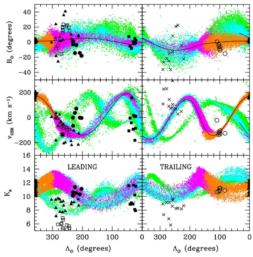
The agreement between the apparent magnitudes of the -body model and the Monaco et al. (2007) data appears to be relatively good. Unfortunately it is difficult to evaluate this agreement for the Chou et al. (2007) data since these authors focussed on the brightest available M-giants, which are expected to be biased several or more brighter than the mean for the stream (see discussion by Chou et al. 2009). A more instructive comparison is to the M-giant survey of Majewski et al. (2003). In Figure 18 we plot the apparent magnitude for the simulated Sgr dwarf, overlaid with the original M-giant sample from Majewski et al. (2003; i.e., similar to their Fig. 8) and the subsample with radial velocity data which we culled from Law et al. (2004) and Majewski et al. (2004) in Figure 1 (open boxes in Figure 18). The magnitudes derived from the model match the larger M-giant sample of the dynamically young sections of the tidal streams (i.e., for the trailing arm, and for the leading arm) well: Over 95% of the radial velocity subsample have magnitudes consistent with the -body model. The remaining 5% may be Galactic interlopers at smaller distances whose colors and radial velocities happened to be coincident with those of the Sgr stream, although a few located around may be associated with the T1 wrap of the trailing arm stream instead of the fainter (and more distant) L1 stream since the radial velocity trends of the L1 and T1 wraps are expected to cross in this region of the sky.
There are a few regions of stars in Figure 18 that are not explained by the model however. In particular there is a distribution of M-giants at at all orbital longitudes that are not reproduced by the -body model. At these faint M-giants arguably appear to join smoothly to the trailing arm trend (see also Newberg et al. 2003), suggesting (Pakzad et al. 2004) that the trailing arm may not turn around at this location to approach closer to the Sun again (as the -body model does) but instead forms a wrap around the entire sky at relatively constant . Such a wrap is strongly inconsistent with the predictions of all -body models to date and, if genuine, may be evidence for a strong evolution in the orbital path of Sgr Gyr ago.
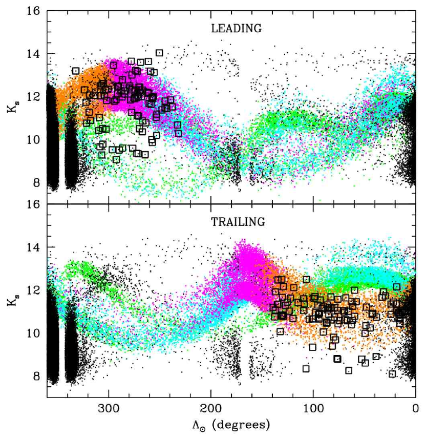
7.4. Caveats
7.4.1 Relation to Other Tracers
The picture presented here of the evolution in the mean metallicity along the Sgr tidal arms is biased towards more metal-rich stars, since it has been fitted to observations of intrinsically metal-rich M-giant tracers. Other tracers such as blue horizontal branch (BHB) stars (e.g., Yanny et al. 2009), RR Lyrae (RRL; Vivas et al. 2005, Prior et al. 2009), or K-giants (Starkenburg et al. 2009; see also Dohm-Palmer et al. 2001) might reasonably be expected to differ from the trends calculated here. It is unclear, however, how stars more metal-poor than (as detected by Yanny et al. 2009) might arise in large numbers in relatively young sections of the Sgr stream (i.e., the L1 arm at ) since no remnants of populations so metal poor remain in the core of Sgr today (Siegel et al. 2007). If this metal-poor stellar population has indeed recently been completely stripped from Sgr it may provide a useful constraint upon future models of the distribution of stellar populations within the initial Sgr dSph. We discuss this issue further in §8.
7.4.2 Uniqueness
The fact that we have been able to find a method for tagging particles in the initial satellite to correspond to the stellar populations seen in the tidal streams should not be taken to mean that this structure of the initial satellite is uniquely correct, that the optimal ranges in found for each star formation episode A-E correspond exactly to the total stellar mass produced in the bursts, or even that the method is a particularly good description of the tidal stripping of specific stellar populations within a real Galactic dSph. The mass loss history of the satellite is a strong function of the adopted model, and different values for the total mass, scale length, or interaction time of the dwarf will produce different amounts of overlap between various eras of tidal debris, and various ranges in orbital energy within the original dwarf. Similarly, if we were to adopt a different physical model for Sgr (e.g., a cuspy Hernquist profile, or a more physically motivated two-component King-profile stellar core combined with an extended NFW dark matter halo), or consider the possible conversion of an originally disky dwarf to a dSph via tidal stirring (e.g., Mayer et al. 2006) the mass loss history could also be very different (see, e.g., Read et al. 2006ab). The specific distribution and mass normalization of individual stellar populations is therefore contingent on the adopted model and should not be interpreted as a general result, but can be refined as more observational data become available.
8. Discussion: Relation to Possible Detections of Sgr Tidal Debris
The model presented in this paper has the attractive quality that it provides a reasonable match to the major dynamical characteristics of Sgr tidal debris measured from wide-field surveys. It is worthwhile also investigating the degree of correspondence between the -body model and various narrow-field observations of subgiant stars, K-giants, and RRL that have been postulated to trace the Sgr tidal stream.
In Figure 19 we plot the -body model of the Sgr stream overlaid by a selection of detections from recent narrow-field surveys (this comparison is not exhaustive, see also discussion by Majewski et al. 2003). We discuss each data set in detail below. Note that we do not consider possible associations with globular clusters or faint dwarf satellites; these are treated separately in a forthcoming contribution (Law et al. in prep.).
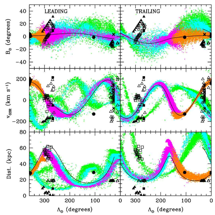
8.1. SDSS Stripe 82
Cole et al. (2008) used a maximum likelihood method to characterize the spatial properties of F-turnoff stars in stripe 82 of the SDSS. They observed tidal debris located at , corresponding to Sgr longitudinal coordinates . As illustrated by Figure 19 (filled circles) the T1 wrap of the -body model is an extremely good match to these F-turnoff stars in both angular position and distance (matching to within in , and 1 kpc in distance). Cole et al. (2008) measured the width of the stream perpendicular to the line of sight at this to have a FWHM kpc. The -body stream is slightly fatter with FWHM kpc, but given the single component mass-follows-light model employed for Sgr the agreement with the apparent width of a specific stellar population is extremely good.
The radial velocity of a sample of RRL in Stripe 82 has recently been measured by Watkins et al. (2009), who detect a component with km s, which is matched by the mean radial velocity of the T1 stream at this position to within 5 km s. Watkins et al. (2009) also measure the metallicity of these RRL, finding that . This value is appreciably more metal-poor than either the M-giant sample or the mean of the -body model at this longitude (). This difference in measured metallicity emphasizes the strong sensitivity of derived metallicities of a stellar stream to the biases imposed by the type of stellar tracer used (e.g., metal-poor populations do not generally form M giants while metal-rich populations do not generally form RRL). Thus, until an unbiased assessment of the MDF along the Sgr stream is obtained, models such as that presented in §7, which was constrained by a single type of metallicity-biased population tracer, must be considered as merely a demonstration of how MDF-variations can originate.
8.2. RRL and K-giants at
Vivas et al. (2005) published VLT spectroscopy of 16 RRL from the QUEST survey in the range . All but 1-2 of these stars, (which have highly discrepant velocities, at and km s) are in agreement with the angular position, distance and radial velocity trend of the L1 arm of the -body model (see Figure 19, open boxes). Starkenburg et al. (2009) have also detected an overdensity of 5 K-giant stars at similar orbital longitude that are well-matched to the distance and radial velocity of the -body model stream (Figure 19, skeletal triangles), although they appear to be located towards the edge of the stream in .171717Note that the star added to the Starkenburg et al. (2009) group using the ‘4dist’ criterion is not as well-matched to the -body stream as the other 5 stars, with the former discrepant by km s.
Both samples of stars are well-reproduced by the -body model, although we note that the Vivas et al. (2005) and Starkenburg et al. (2009) samples have mean metallicity and respectively. These metallicities are entirely consistent with each other, but significantly more metal-poor than the M-giant sample, which has . As was the case for SDSS Stripe 82, this reinforces the conclusion that stellar populations significantly more metal-poor than the M-giant subsample exist at a range of orbital longitudes throughout the Sgr tidal streams. As expected on the basis of dynamical age, the RRL of Vivas et al. (2005) which correspond to tidal debris Gyr old (i.e., magenta points in Figure 19) are slightly more metal-poor than the RRL in SDSS Stripe 82 which correspond to Gyr old debris.
We note that an additional sample of metal-poor K-giant stars in a similar longitude range was also pointed out by Kundu et al. (2002; filled triangles in Figure 19). While the L2/T2 wraps of the -body stream match the radial velocity trend of these stars, the angular positions are discrepant by up to for L2 and for T2. At a typical distance kpc the Kundu et al. (2002) stars are also much closer than expected for the T2 arm ( kpc), but may be consistent with the L2 arm ( kpc). If these stars genuinely belong to the Sgr stream, it is most likely that they belong to the L2 wrap, and may suggest that the angular coordinates and/or distance of this wrap in the -body model require adjustment.
8.3. Virgo: The VSS and the VOD
Recent years have witnessed a wealth of substructure discovered in the direction of Virgo, which we follow Martínez-Delgado et al. (2007) in classifying into the Virgo Stellar Stream (VSS) and the Virgo Overdensity (VOD).
The VSS (as traced by QUEST RRL; Duffau et al. 2006) is a relatively well-defined feature that lies at an angular position , i.e., projected on the outer edge of the L1/L2 streams and significantly off the T1/T2 streams in sky position. At a distance of 19 kpc, it is roughly coincident with the L2/T1 stream, but has a radial velocity ( km s; Duffau et al. 2006) that is discrepant with these wraps by 220/94 km srespectively. Curiously, the proper motion of the VSS (; Casetti-Dinescu et al. 2009) is reproduced by the T1 stream to within (), but given the angular position and radial velocity mismatch we conclude that the VSS is unlikely to be associated with the Sgr stream.
In contrast, the VOD (Jurić et al. 2008) is a much less well-defined, diffuse clump of stars around that covers more than deg2 on the sky. The possible association of the VOD with Sgr has been addressed in detail by Martínez-Delgado et al. (2007), who noted that it was roughly coincident with tidal debris from models of the Sgr dwarf (LJM05) disrupting in an axisymmetric, oblate Galactic halo.
In the triaxial halo model derived in this contribution, we find that the model Sgr stream arcs significantly over the solar neighborhood, and tidal debris in the L1 tidal stream at the angular coordinates of the VOD lies much too far away ( kpc for the Sgr stream versus kpc for the VOD) to be associated (see Figure 19, filled squares). Similarly, both the T1 and T2 wraps lie too far away to produce the VOD, in addition to lying in the opposite angular direction .
Interestingly, this angular position and distance does correspond closely to the predicted location of the secondary L2 wrap of leading Sgr tidal debris, suggesting that the VOD may be evidence for old tidal debris torn from Sgr Gyr ago. If such an identification is correct, we should expect the radial velocity of the VOD to be km s. Recent observational work on QUEST RRL in the direction of the VOD by Vivas et al. (2008) derived radial velocity signatures at km s. The first (and by far most significant) two of these velocity structures are strongly discrepant with the expected signal by and km srespectively. The third structure is possibly consistent with the velocity signature expected of the L2 Sgr stream, differing by only km sin this part of the simulated debris where the -body stream is ill-constrained. Only 7% of the QUEST RRL (i.e., 3/43) are contained in this km svelocity structure however, and we therefore concur with the conclusion of Vivas et al. (2008) that while Sgr may make some minor contribution to the VOD it is not the dominant origin of the stellar overdensity.
8.4. SEKBO RRL
An additional sample of RRL stars from the SEKBO (Moody et al. 2003) survey has recently been studied by Keller et al. (2008), with radial velocities presented by Prior et al. (2009). The Prior et al. (2009) subsample focuses on two groups of RRL which they group into the “VSS region” at hr (i.e., ) and the “Sgr region” at hr (i.e., ). These two groups of stars are plotted against our -body model in Figure 19 (open triangles).
Considering first the angular coordinate plot vs. , we note that neither of these groups of stars are well-centered on the predicted path of the -body tidal stream, lying at the extreme outer edge of the L1/L2 streams and fully outside the angular path of the T1/T2 streams. This is consistent with Figure 15 of Keller et al. (2008): The plane of the SEKBO survey intersects the Sgr plane at an angle and best overlaps at h (i.e., behind the Galactic Center) and h. In the regions traced by the Prior et al. (2009) subsample we confirm that the RRL tend to lie away from the bulk of the Sgr stream. It is perhaps unsurprising then that the distances (typically 16-21 kpc) and radial velocities of the RRL do not obviously match any particular branch of the Sgr stream. While Prior et al. (2009) discussed a possible match between some RRL and trailing Sgr tidal debris in the oblate-halo model of LJM05, no such match obviously exists for the updated model presented here.
We note that the distance ( kpc) and radial velocity range ( - km s) of the sample of Prior et al. (2009) is similar to that found for a sample of red clump stars by Majewski et al. (1999; crosses in Figure 19). These red clump stars lie near the angular position of the L1 stream, and LJM05 discussed the possibility that their large spread in radial velocities may indicate the range of velocities occupied by the Sgr stream at this longitude. Given the similarities in distance and radial velocity of the Prior et al. (2009) and Majewski et al. (1999) samples, it is at least likely that they trace the same Galactic substructure. If this substructure is confirmed to be the Sgr stream, it will suggest that the L1 stream at has a greater angular width, smaller distance, and larger spread in radial velocities than predicted by the current -body model.
8.5. Subgiant Populations in the Leading Tidal Stream
Keller (2009) has recently described a population of subgiant stars in the range from the SDSS that may correspond to the L1 stream of Sgr. While this paper gives insufficient information to include these stars in Figure 19, we note that the vs distance trend illustrated in Figure 7 of Keller (2009) is reproduced by the revised -body model to within kpc, in contrast to previous -body models of the Sgr stream (e.g., LJM05). Further characterization of this subgiant population may therefore provide even greater insight into the nature of the Sgr leading tidal stream.
9. Summary
We have presented the first numerical model of the Sgr — Milky Way system that is capable of simultaneously satisfying the majority of major constraints on the angular positions, distances, and radial velocities of the dynamically young tidal debris streams. In particular, we have resolved the so-called “halo conundrum”, whereby models were previously incapable of fitting both the angular position and distance/radial velocity trends of leading tidal debris. The publically-available -body model also makes concrete predictions for the location and kinematics of older tidal debris not yet conclusively observed in the Galactic halo. Future observational evidence for the presence/absence of such streams will place strong constraints on the total interaction time of the dSph with the Milky Way.
The key ingredient in the success of this model is our introduction of a non-axisymmetric component to the Galactic gravitational potential, in the form of a nearly oblate dark matter halo with axial ratios whose minor axis lies within the plane of the Galactic disk plane within of the line connecting the Sun and the Galactic center. While this inclined-halo explanation permits the model to reproduce the observational data, it is not strongly motivated within the current CDM paradigm, and may simply serve as a numerical crutch that mimics the effect of some as-yet unidentified alternative (such as Sgr orbital evolution or the gravitational influence of the Magellanic Clouds).
Our -body model suggests that Sgr has been orbiting in the gravitational potential of the Milky Way for at least 3 Gyr and consists of a remaining bound mass . The total space velocity of Sgr is predicted to be km s, which at a distance kpc corresponds to an apparent proper motion of mas yr-1 and a radial velocity of 142 km sin the heliocentric rest frame. In contrast to some previous models, the Sgr stream is not expected to approach the solar position to closer than kpc. We have additionally demonstrated that it is possible to understand the observed evolution of the MDF along the Sgr tidal streams in terms of the dynamical superposition of stars formed in multiple bursts of star formation and torn from the satellite at different times, suggesting that the chemical abundances of stars in Sgr at the present day may be significantly different than the abundances of those contributed to the Galactic stellar halo.
Despite our success in fitting the strongest observational constraints on the primary wraps of the leading and trailing tidal arms, it is uncertain what gives rise to the low surface brightness, high-declination ‘bifurcation’ of the stream that parallels the leading arm at higher declination in the SDSS footprint. We postulate that substructure or anisotropic internal dynamics within the progenitor satellite may cause the observed bifurcation, indicating that future numerical models of the Sgr stream must explore the influence of the internal dynamics of the progenitor on the subsequently formed tidal tails. Such models must include realistic treatments of the dark and baryonic material as separate components and explore both rotation and orbital anisotropy of the visible matter. Moreover, the effects of evolution in the Sgr orbit and the peturbative gravitational influence of Milky Way substructures such as the LMC must be investigated in greater detail.
References
- Adams et al. (2007) Adams, F. C., Bloch, A. M., Butler, S. C., Druce, J. M., & Ketchum, J. A. 2007, ApJ, 670, 1027
- Allgood et al. (2006) Allgood, B., Flores, R. A., Primack, J. R., Kravtsov, A. V., Wechsler, R. H., Faltenbacher, A., & Bullock, J. S. 2006, MNRAS, 367, 1781
- Babusiaux & Gilmore (2005) Babusiaux, C., & Gilmore, G. 2005, MNRAS, 358, 1309
- Bailin & Steinmetz (2005) Bailin, J., & Steinmetz, M. 2005, ApJ, 627, 647
- Bekenstein (2004) Bekenstein, J. D. 2004, Phys. Rev. D, 70, 083509
- Bell et al. (2008) Bell, E. F., et al. 2008, ApJ, 680, 295
- Bellazzini et al. (2006) Bellazzini, M., Newberg, H. J., Correnti, M., Ferraro, F. R., & Monaco, L. 2006, A&A, 457, L21
- Belokurov et al. (2006) Belokurov, V., et al. 2006, ApJ, 642, L137
- Belokurov et al. (2007) Belokurov, V., et al. 2007, ApJ, 658, 337
- Besla et al. (2007) Besla, G., Kallivayalil, N., Hernquist, L., Robertson, B., Cox, T. J., van der Marel, R. P., & Alcock, C. 2007, ApJ, 668, 949
- Bett et al. (2009) Bett, P., Eke, V., Frenk, C. S., Jenkins, A., & Okamoto, T. 2009, arXiv:0906.2785
- Blitz & Spergel (1991) Blitz, L., & Spergel, D. N. 1991, ApJ, 379, 631
- Bullock et al. (2001) Bullock, J. S., Dekel, A., Kolatt, T. S., Kravtsov, A. V., Klypin, A. A., Porciani, C., & Primack, J. R. 2001a, ApJ, 555, 240
- Bullock et al. (2001) Bullock, J. S., Kravtsov, A. V., & Weinberg, D. H. 2001b, ApJ, 548, 33
- Bullock (2002) Bullock, J. S. 2002, The Shapes of Galaxies and their Dark Halos, 109
- Bullock & Johnston (2005) Bullock, J. S., & Johnston, K. V. 2005, ApJ, 635, 931
- Buote et al. (2002) Buote, D. A., Jeltema, T. E., Canizares, C. R., & Garmire, G. P. 2002, ApJ, 577, 183
- Casetti-Dinescu et al. (2009) Casetti-Dinescu, D. I., Girard, T. M., Majewski, S. R., Vivas, A. K., Wilhelm, R., Carlin, J. L., Beers, T. C., & van Altena, W. F. 2009, ApJ, 701, L29
- Chabrier (2001) Chabrier, G. 2001, ApJ, 554, 1274
- Choi et al. (2007) Choi, J.-H., Weinberg, M. D., & Katz, N. 2007, MNRAS, 381, 987
- Chou et al. (2007) Chou, M.-Y., et al. 2007, ApJ, 670, 346
- Chou et al. (2009) Chou, M.-Y., Cunha, K., Majewski, S. R., Smith, V. V., Patterson, R. J., Martinez-Delgado, D., & Geisler, D. 2009, arXiv:0911.4364
- Cole et al. (2008) Cole, N., et al. 2008, ApJ, 683, 750
- Corless et al. (2009) Corless, V. L., King, L. J., & Clowe, D. 2009, MNRAS, 393, 1235
- Debattista et al. (2008) Debattista, V. P., Moore, B., Quinn, T., Kazantzidis, S., Maas, R., Mayer, L., Read, J., & Stadel, J. 2008, ApJ, 681, 1076
- Dehnen & Binney (1998) Dehnen, W., & Binney, J. 1998, MNRAS, 294, 429
- Diehl & Statler (2007) Diehl, S., & Statler, T. S. 2007, ApJ, 668, 150
- Diemand et al. (2007) Diemand, J., Kuhlen, M., & Madau, P. 2007, ApJ, 657, 262
- Dinescu et al. (2002) Dinescu, D. I., et al. 2002, ApJ, 575, L67
- Dinescu et al. (2005) Dinescu, D. I., Girard, T. M., van Altena, W. F., & López, C. E. 2005, ApJ, 618, L25
- Dohm-Palmer et al. (2001) Dohm-Palmer, R. C., et al. 2001, ApJ, 555, L37
- Duffau et al. (2006) Duffau, S., Zinn, R., Vivas, A. K., Carraro, G., Méndez, R. A., Winnick, R., & Gallart, C. 2006, ApJ, 636, L97
- Edelsohn & Elmegreen (1997) Edelsohn, D. J., & Elmegreen, B. G. 1997, MNRAS, 290, 7
- Evans & Bridle (2009) Evans, A. K. D., & Bridle, S. 2009, ApJ, 695, 1446
- Eyre & Binney (2009) Eyre, A., & Binney, J. 2009, MNRAS, 400, 548
- Fellhauer et al. (2006) Fellhauer, M., et al. 2006, ApJ, 651, 167
- Flores et al. (2007) Flores, R. A., Allgood, B., Kravtsov, A. V., Primack, J. R., Buote, D. A., & Bullock, J. S. 2007, MNRAS, 377, 883
- Font et al. (2001) Font, A. S., Navarro, J. F., Stadel, J., & Quinn, T. 2001, ApJ, 563, L1
- Font et al. (2006) Font, A. S., Johnston, K. V., Bullock, J. S., & Robertson, B. E. 2006, ApJ, 638, 585
- Fusi Pecci et al. (1995) Fusi Pecci, F., Bellazzini, M., Cacciari, C., & Ferraro, F. R. 1995, AJ, 110, 1664
- Geisler et al. (2005) Geisler, D., Smith, V. V., Wallerstein, G., Gonzalez, G., & Charbonnel, C. 2005, AJ, 129, 1428
- Gerhard & Vietri (1986) Gerhard, O. E., & Vietri, M. 1986, MNRAS, 223, 377
- Gnedin et al. (2005) Gnedin, O. Y., Gould, A., Miralda-Escudé, J., & Zentner, A. R. 2005, ApJ, 634, 344
- Gómez-Flechoso et al. (1999) Gómez-Flechoso, M. A., Fux, R., & Martinet, L. 1999, A&A, 347, 77
- Grillmair & Dionatos (2006) Grillmair, C. J., & Dionatos, O. 2006, ApJ, 641, L37
- Groenewegen et al. (2008) Groenewegen, M. A. T., Udalski, A., & Bono, G. 2008, A&A, 481, 441
- Hayashi et al. (2007) Hayashi, E., Navarro, J. F., & Springel, V. 2007, MNRAS, 377, 50
- Helmi et al. (1999) Helmi, A., White, S. D. M., de Zeeuw, P. T., & Zhao, H. 1999, Nature, 402, 53
- Helmi (2004) Helmi, A. 2004, ApJ, 610, L97
- Helmi & White (2001) Helmi, A., & White, S. D. M. 2001, MNRAS, 323, 529
- Herbert-Fort et al. (2007) Herbert-Fort, S., Zaritsky, D., Kim, Y. J., Bailin, J., & Taylor, J. E. 2007, IAU Symposium, 235, 104
- Herbert-Fort et al. (2008) Herbert-Fort, S., Zaritsky, D., Jin Kim, Y., Bailin, J., & Taylor, J. E. 2008, MNRAS, 384, 803
- Hernquist & Ostriker (1992) Hernquist, L., & Ostriker, J. P. 1992, ApJ, 386, 375
- Hoekstra et al. (2004) Hoekstra, H., Yee, H. K. C., & Gladders, M. D. 2004, ApJ, 606, 67
- Ibata et al. (1994) Ibata, R. A., Gilmore, G., & Irwin, M. J. 1994, Nature, 370, 194
- Ibata et al. (1997) Ibata, R. A., Wyse, R. F. G., Gilmore, G., Irwin, M. J., & Suntzeff, N. B. 1997, AJ, 113, 634
- Ibata et al. (2001) Ibata, R., Irwin, M., Lewis, G., Ferguson, A. M. N., & Tanvir, N. 2001a, Nature, 412, 49
- Ibata et al. (2001) Ibata, R., Lewis, G. F., Irwin, M., Totten, E., & Quinn, T. 2001b, ApJ, 551, 294
- Ibata et al. (2003) Ibata, R. A., Irwin, M. J., Lewis, G. F., Ferguson, A. M. N., & Tanvir, N. 2003, MNRAS, 340, L21
- Iodice et al. (2003) Iodice, E., Arnaboldi, M., Bournaud, F., Combes, F., Sparke, L. S., van Driel, W., & Capaccioli, M. 2003, ApJ, 585, 730
- Irwin et al. (1996) Irwin, M., Ibata, R., Gilmore, G., Wyse, R., & Suntzeff, N. 1996, Formation of the Galactic Halo…Inside and Out, 92, 84
- Jing & Suto (2002) Jing, Y. P., & Suto, Y. 2002, ApJ, 574, 538
- Johnston et al. (1995) Johnston, K. V., Spergel, D. N., & Hernquist, L. 1995, ApJ, 451, 598
- Johnston et al. (1996) Johnston, K. V., Hernquist, L., & Bolte, M. 1996, ApJ, 465, 278
- Johnston (1998) Johnston, K. V. 1998, ApJ, 495, 297
- Johnston et al. (1999) Johnston, K. V., Majewski, S. R., Siegel, M. H., Reid, I. N., & Kunkel, W. E. 1999, AJ, 118, 1719
- Johnston et al. (2005) Johnston, K. V., Law, D. R., & Majewski, S. R. 2005, ApJ, 619, 800
- Jurić et al. (2008) Jurić, M., et al. 2008, ApJ, 673, 864
- Kalberla et al. (2005) Kalberla, P. M. W., Burton, W. B., Hartmann, D., Arnal, E. M., Bajaja, E., Morras, R., Poeppel, W. G. L. 2005, A&A, 440, 775
- Kalirai et al. (2006) Kalirai, J. S., Guhathakurta, P., Gilbert, K. M., Reitzel, D. B., Majewski, S. R., Rich, R. M., & Cooper, M. C. 2006, ApJ, 641, 268
- Kazantzidis et al. (2004) Kazantzidis, S., Kravtsov, A. V., Zentner, A. R., Allgood, B., Nagai, D., & Moore, B. 2004, ApJ, 611, L73
- Keller et al. (2008) Keller, S. C., Murphy, S., Prior, S., Da Costa, G., & Schmidt, B. 2008, ApJ, 678, 851
- Keller (2009) Keller, S. C. 2009, arXiv:0911.0951
- Koposov et al. (2009) Koposov, S. E., Rix, H.-W., & Hogg, D. W. 2009, arXiv:0907.1085
- Kuhlen et al. (2007) Kuhlen, M., Diemand, J., & Madau, P. 2007, ApJ, 671, 1135
- Kunder & Chaboyer (2009) Kunder, A., & Chaboyer, B. 2009, AJ, 137, 4478
- Kundu et al. (2002) Kundu, A., et al. 2002, ApJ, 576, L125
- Kunkel & Demers (1976) Kunkel, W. E., & Demers, S. 1976, The Galaxy and the Local Group, 182, 241
- Larsen & Humphreys (1996) Larsen, J. A., & Humphreys, R. M. 1996, ApJ, 468, L99
- Law et al. (2004) Law, D. R., Majewski, S. R., Skrutskie, M. F., & Johnston, K. V. 2004, Satellites and Tidal Streams, 327, 239
- Law et al. (2005) Law, D. R., Johnston, K. V., & Majewski, S. R. 2005, ApJ, 619, 807 (LJM05)
- Law et al. (2009) Law, D. R., Majewski, S. R., & Johnston, K. V. 2009, ApJ, 703, L67 (LMJ09)
- Lee & Suto (2003) Lee, J., & Suto, Y. 2003, ApJ, 585, 151
- Lynden-Bell (1982) Lynden-Bell, D. 1982, The Observatory, 102, 202
- Majewski (1993) Majewski, S. R. 1993, ARA&A, 31, 575
- Majewski (1994) Majewski, S. R. 1994, ApJ, 431, L17
- Majewski et al. (1996) Majewski, S. R., Munn, J. A., & Hawley, S. L. 1996, ApJ, 459, L73
- Majewski et al. (1999) Majewski, S. R., Siegel, M. H., Kunkel, W. E., Reid, I. N., Johnston, K. V., Thompson, I. B., Landolt, A. U., & Palma, C. 1999, AJ, 118, 1709
- Majewski et al. (2002) Majewski, S. R., et al. 2002, Modes of Star Formation and the Origin of Field Populations, 285, 199
- Majewski et al. (2003) Majewski, S. R., Skrutskie, M. F., Weinberg, M. D., & Ostheimer, J. C. 2003, ApJ, 599, 1082
- Majewski (2004) Majewski, S. R. 2004, Publications of the Astronomical Society of Australia, 21, 197
- Majewski et al. (2004) Majewski, S. R., et al. 2004, AJ, 128, 245
- Majewski et al. (2006) Majewski, S. R., Law, D. R., Polak, A. A., & Patterson, R. J. 2006, ApJ, 637, L25
- Mandelbaum et al. (2006) Mandelbaum, R., Hirata, C. M., Broderick, T., Seljak, U., & Brinkmann, J. 2006, MNRAS, 370, 1008
- Marigo et al. (2008) Marigo, P., Girardi, L., Bressan, A., Groenewegen, M. A. T., Silva, L., & Granato, G. L. 2008, A&A, 482, 883
- Martínez-Delgado et al. (2004) Martínez-Delgado, D., Gómez-Flechoso, M. Á., Aparicio, A., & Carrera, R. 2004, ApJ, 601, 242
- Martínez-Delgado et al. (2007) Martínez-Delgado, D., Peñarrubia, J., Jurić, M., Alfaro, E. J., & Ivezić, Z. 2007, ApJ, 660, 1264
- Martínez-Delgado et al. (2008) Martínez-Delgado, D., Peñarrubia, J., Gabany, R. J., Trujillo, I., Majewski, S. R., & Pohlen, M. 2008, ApJ, 689, 184
- Martínez-Delgado et al. (2009) Martínez-Delgado, D., Pohlen, M., Gabany, R. J., Majewski, S. R., Peñarrubia, J., & Palma, C. 2009, ApJ, 692, 955
- Mayer et al. (2006) Mayer, L., Mastropietro, C., Wadsley, J., Stadel, J., & Moore, B. 2006, MNRAS, 369, 1021
- McConnachie et al. (2003) McConnachie, A. W., Irwin, M. J., Ibata, R. A., Ferguson, A. M. N., Lewis, G. F., & Tanvir, N. 2003, MNRAS, 343, 1335
- Metz et al. (2007) Metz, M., Kroupa, P., & Jerjen, H. 2007, MNRAS, 374, 1125
- Metz et al. (2009) Metz, M., Kroupa, P., & Jerjen, H. 2009, MNRAS, 394, 2223
- Milgrom (1983) Milgrom, M. 1983, ApJ, 270, 365
- Miyamoto & Nagai (1975) Miyamoto, M., & Nagai, R. 1975, PASJ, 27, 533
- Monaco et al. (2007) Monaco, L., Bellazzini, M., Bonifacio, P., Buzzoni, A., Ferraro, F. R., Marconi, G., Sbordone, L., & Zaggia, S. 2007, A&A, 464, 201
- Monaco et al. (2005) Monaco, L., Bellazzini, M., Ferraro, F. R., & Pancino, E. 2005, MNRAS, 356, 1396
- Moody et al. (2003) Moody, R., Schmidt, B., Alcock, C., Goldader, J., Axelrod, T., Cook, K. H., & Marshall, S. 2003, Earth Moon and Planets, 92, 125
- Morris & Serabyn (1996) Morris, M., & Serabyn, E. 1996, ARA&A, 34, 645
- Muñoz et al. (2006) Muñoz, R. R., et al. 2006, ApJ, 649, 201
- Nakada et al. (1991) Nakada, Y., Onaka, T., Yamamura, I., Deguchi, S., Hashimoto, O., Izumiura, H., & Sekiguchi, K. 1991, Nature, 353, 140
- Narayan et al. (2005) Narayan, C. A., Saha, K., & Jog, C. J. 2005, A&A, 440, 523
- Navarro et al. (1996) Navarro, J. F., Frenk, C. S., & White, S. D. M. 1996, ApJ, 462, 563
- Newberg et al. (2002) Newberg, H. J., et al. 2002, ApJ, 569, 245
- Newberg et al. (2003) Newberg, H. J., et al. 2003, ApJ, 596, L191
- Newberg & Yanny (2006) Newberg, H. J., & Yanny, B. 2006, Journal of Physics Conference Series, 47, 195
- Newberg et al. (2007) Newberg, H. J., Yanny, B., Cole, N., Beers, T. C., Re Fiorentin, P., Schneider, D. P., & Wilhelm, R. 2007, ApJ, 668, 221
- Newberg et al. (2009) Newberg, H. J., Yanny, B., & Willett, B. A. 2009, ApJ, 700, L61
- Nidever et al. (2008) Nidever, D. L., Majewski, S. R., & Burton, W. B. 2008, ApJ, 679, 432
- Odenkirchen et al. (2009) Odenkirchen, M., Grebel, E. K., Kayser, A., Rix, H.-W., & Dehnen, W. 2009, AJ, 137, 3378
- Olling & Merrifield (2000) Olling, R. P., & Merrifield, M. R. 2000, MNRAS, 311, 361
- Pakzad et al. (2004) Pakzad, S. L., et al. 2004, Bulletin of the American Astronomical Society, 36, 1582
- Peñarrubia et al. (2005) Peñarrubia, J., et al. 2005, ApJ, 626, 128
- Peñarrubia et al. (2006) Peñarrubia, J., Benson, A. J., Martínez-Delgado, D., & Rix, H. W. 2006, ApJ, 645, 240
- Peñarrubia et al. (2008) Peñarrubia, J., Navarro, J. F., & McConnachie, A. W. 2008, ApJ, 673, 226
- Peñarrubia et al. (2009) Peñarrubia, J., Navarro, J. F., McConnachie, A. W., & Martin, N. F. 2009, ApJ, 698, 222
- Perets et al. (2009) Perets, H. B., Wu, X., Zhao, H. S., Famaey, B., Gentile, G., & Alexander, T. 2009, ApJ, 697, 2096
- Plummer (1911) Plummer, H. C. 1911, MNRAS, 71, 460
- Prior et al. (2009) Prior, S. L., Da Costa, G. S., & Keller, S. C. 2009, ApJ, 704, 1327
- Pryor et al. (2010) Pryor, C., Piatek, S., & Olszewski, E. W. 2010, AJ, 139, 839
- Putman et al. (2004) Putman, M. E., Thom, C., Gibson, B. K., & Staveley-Smith, L. 2004, ApJ, 603, L77
- Read & Moore (2005) Read, J. I., & Moore, B. 2005, MNRAS, 361, 971
- Read et al. (2006a) Read, J. I., Wilkinson, M. I., Evans, N. W., Gilmore, G., & Kleyna, J. T. 2006a, MNRAS, 366, 429
- Read et al. (2006b) Read, J. I., Wilkinson, M. I., Evans, N. W., Gilmore, G., & Kleyna, J. T. 2006b, MNRAS, 367, 387
- Reid (1993) Reid, M. J. 1993, ARA&A, 31, 345
- Reid & Brunthaler (2004) Reid, M. J., & Brunthaler, A. 2004, ApJ, 616, 872
- Rocha-Pinto et al. (2004) Rocha-Pinto, H. J., Majewski, S. R., Skrutskie, M. F., Crane, J. D., & Patterson, R. J. 2004, ApJ, 615, 732
- Rŭžička et al. (2007) Rŭžička, A., Palouš, J., & Theis, C. 2007, A&A, 461, 155
- Saha et al. (2009) Saha, K., Levine, E. S., Jog, C. J., & Blitz, L. 2009, ApJ, 697, 2015
- Sakamoto et al. (2003) Sakamoto, T., Chiba, M., & Beers, T. C. 2003, A&A, 397, 899
- Seabroke et al. (2008) Seabroke, G. M., et al. 2008, MNRAS, 384, 11
- Searle & Zinn (1978) Searle, L., & Zinn, R. 1978, ApJ, 225, 357
- Shang et al. (1998) Shang, Z., et al. 1998, ApJ, 504, L23
- Siegel et al. (2007) Siegel, M. H., et al. 2007, ApJ, 667, L57
- Starkenburg et al. (2009) Starkenburg, E., et al. 2009, ApJ, 698, 567
- Tolstoy et al. (2004) Tolstoy, E., et al. 2004, ApJ, 617, L119
- Totten & Irwin (1998) Totten, E. J., & Irwin, M. J. 1998, MNRAS, 294, 1
- Valluri et al. (2009) Valluri, M., Debattista, V. P., Quinn, T., & Moore, B. 2009, arXiv:0906.4784
- van den Bosch et al. (2002) van den Bosch, F. C., Abel, T., Croft, R. A. C., Hernquist, L., & White, S. D. M. 2002, ApJ, 576, 21
- van der Marel et al. (2002) van der Marel, R. P., Alves, D. R., Hardy, E., & Suntzeff, N. B. 2002, AJ, 124, 2639
- Velazquez & White (1995) Velazquez, H., & White, S. D. M. 1995, MNRAS, 275, L23
- Vivas et al. (2005) Vivas, A. K., Zinn, R., & Gallart, C. 2005, AJ, 129, 189
- Vivas et al. (2008) Vivas, A. K., Jaffé, Y. L., Zinn, R., Winnick, R., Duffau, S., & Mateu, C. 2008, AJ, 136, 1645
- Warren et al. (1992) Warren, M. S., Quinn, P. J., Salmon, J. K., & Zurek, W. H. 1992, ApJ, 399, 405
- Watkins et al. (2009) Watkins, L. L., et al. 2009, MNRAS, 398, 1757
- Weinberg (1998) Weinberg, M. D. 1998, MNRAS, 299, 499
- Widrow (2008) Widrow, L. M. 2008, ApJ, 679, 1232
- Wu et al. (2008) Wu, X., Famaey, B., Gentile, G., Perets, H., & Zhao, H. 2008, MNRAS, 386, 2199
- Xu et al. (2006) Xu, Y., Deng, L. C., & Hu, J. Y. 2006, MNRAS, 368, 1811
- Yanny et al. (2009) Yanny, B., et al. 2009, ApJ, 700, 1282
- Yu & Madau (2007) Yu, Q., & Madau, P. 2007, MNRAS, 379, 1293
- Zentner et al. (2005) Zentner, A. R., Kravtsov, A. V., Gnedin, O. Y., & Klypin, A. A. 2005, ApJ, 629, 219
- Zypman et al. (2005) Zypman, F.R. 2006, American Journal of Physics, Volume 74, Issue 4, pp 295-300.