Exciton diffusion in air-suspended single-walled carbon nanotubes

Abstract

Direct measurements of the diffusion length of excitons in air-suspended single-walled carbon nanotubes are reported. Photoluminescence microscopy is used to identify individual nanotubes and to determine their lengths and chiral indices. Exciton diffusion length is obtained by comparing the dependence of photoluminescence intensity on the nanotube length to numerical solutions of diffusion equations. We find that the diffusion length in these clean, as-grown nanotubes is significantly longer than those reported for micelle-encapsulated nanotubes.

Optical properties of single-walled carbon nanotubes (SWCNTs) are of importance because of their potential applications in nanoscale photonics and optoelectronics Avouris:2008 , and exhibit interesting physics that are unique to one-dimensional systems. Limited screening of Coulomb interaction in SWCNTs causes electron-hole pairs to form excitons with large binding energies Wang:2005 , and these excitons play a central role in optical processes. There exists an upper limit to the exciton density in SWCNTs Murakami:2009 ; Xiao:2010 caused by exciton-exciton annihilation Wang:2004 ; Ma:2005 ; Matsuda:2008 . Since the annihilation rate is determined by exciton diffusion Murakami:2009 ; Russo:2006 ; Luer:2009 , its elucidation is a key to understanding light emission processes and their efficiencies in SWCNTs.

Exciton diffusion is typically characterized by the diffusion length $L=\sqrt{D\tau}$ where $D$ is the diffusion coefficient and $\tau$ is the exciton lifetime. Stepwise quenching of flourescence Cognet:2007 has yielded exciton excursion range $\Lambda=2L=90$ nm, while $L=6$ nm has been reported from time-resolved measurements Luer:2009 . Recent near-field measurement has resulted in $\sqrt{2}L=100$ nm Georgi:2009 . These measurements have been performed on micelle-encapsulated SWCNTs, but it is expected that the transport properties of excitons are extremely sensitive to their surrounding environment. The exciton diffusion length in clean, pristine SWCNTs has the potential to be considerably longer, but the measurements done on suspended $(7,5)$ nanotubes turned out to show $L_{d}=\sqrt{2}L=200$ nm Yoshikawa:2010 .

Here we report direct measurements of the diffusion length of excitons in air-suspended SWCNTs. Individual nanotubes are identified by photoluminescence (PL) imaging, while their lengths and chiral indices are determined by excitation spectroscopy and polarization measurements. With data obtained from 35 individual $(9,8)$ SWCNTs, we are able to extract the exciton diffusion length $L$ by comparing the dependence of PL intensity on the nanotube length with numerical solutions of diffusion equations. We find that the diffusion length is at least 610 nm, which is substantially longer than those reported for micelle-encapsulated SWCNTs Cognet:2007 ; Luer:2009 ; Georgi:2009 . The apparent diffusion length becomes shorter with higher excitation powers, consistent with exciton-exciton annihilation effects.

In order to obtain suspended SWCNTs of various lengths, trenches with widths ranging from 0.4 $\mu$m to 2.0 $\mu$m are prepared on (001) SiO₂/Si substrates. Electron beam lithography and dry etching processes are used to form the trenches, and an additional electron beam lithography step is performed to define catalyst areas next to the trenches. Silica supported Co/Mo catalyst suspended in ethanol is spin-coated and lifted off. SWCNTs are directly grown on these substrates by alcohol catalytic chemical vapor deposition Maruyama:2002 . A scanning electron microscope image of a typical sample is shown in Fig. 1(a). We note that these suspended as-grown SWCNTs are very clean, and exhibit excellent optical and electrical properties Lefebvre:2003 ; Mann:2007 ; Cao:2005 .

A home-built laser-scanning confocal microscope system is used for the PL measurements. In order to excite SWCNTs, an output of a wavelength-tunable continuous-wave Ti:sapphire laser is focused on the sample with a microscope objective lens. PL is collected through a confocal pinhole corresponding to an aperture with 3 $\mu$m diameter at the sample image plane. A fast steering mirror allows lateral scanning of the laser spot for acquiring PL images, and the laser polarization can be rotated with a half-wave plate. PL spectra are collected with a single grating spectrometer and a liquid nitrogen cooled InGaAs photodiode array. All measurements are performed at room temperature in air.

Suspended SWCNTs are identified by taking spectrally resolved PL images. We raster the laser spot across the scan area on the sample and take a PL spectrum at each position. By extracting the emission intensity at the desired emission energy from these PL spectra and replotting it in real space, PL images can be constructed at any spectral position. Typical PL spectra from an individual SWCNT and the substrate are shown in Fig. 1(b). The bright sharp emission line near 0.9 eV is attributed to PL from a suspended SWCNT, while PL from the Si substrate shows a broad peak around 1.1 eV. PL images at emission energies corresponding to the SWCNT [Fig. 1(c)] and Si substrate [Fig. 1(d)] unambiguously show localized SWCNT emission at the trench position. If the nanotube PL position does not coincide with the underlying trench, we exclude those nanotubes from further measurements as they may not be fully suspended. We also exclude nanotubes if they show considerably lower emission intensity as those are likely to have defects or surface contamination.

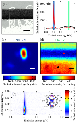
Figure 1: (a) A scanning electron microscope image of a typical sample. The scale bar is 1 $\mu$m. (b) PL spectra for a carbon nanotube (red) and Si substrate (black). Blue and green shades indicate the 4 meV wide integration windows that are used to obtain PL images at emission energies of (c) 0.908 eV and (d) 1.116 eV, respectively. The red and black dots indicate the positions of the laser spot where the red and black curves in (b) were taken, respectively. The scale bars in (c) and (d) are 1 $\mu$m. For (b–d), excitation energy of 1.653 eV and excitation power of 0.36 mW are used. (e) PL excitation map for the same nanotube. Excitation power of 1.5 to 2.5 $\mu$W is used. The spectra are corrected for the changes in excitation power with tuning of the excitation energy. Inset is the laser polarization angle dependence of the PL intensity showing polarization $p=0.90$ for this nanotube. Blue circles are data and the red line is a fit. Taken at an excitation energy of 1.653 eV and an excitation power of 2.24 $\mu$W.

Once we find a suspended SWCNT with bright emission, we perform PL excitation spectroscopy for chirality assignment. As shown in Fig. 1(e), only a single peak is visible throughout the measurement range of excitation and emission energies, and we determine the chirality of this nanotube to be (9,8) from tabulated data Lefebvre:2004apa ; Ohno:2006 . If we find two or more peaks in the PL excitation spectra, those nanotubes are rejected since they may be bundled.

Finally, PL intensity is measured as a function of polarization angle of the excitation laser [Fig. 1(e) inset]. We fit the data to $I_{0}+I_{1}\sin^{2}(\varphi+\varphi_{0})$ where $I_{0}$ and $I_{1}$ are unpolarized and polarized PL intensity, respectively, $\varphi$ is the excitation polarization angle, and $\varphi_{0}$ is the angle offset. From the fit parameters, we compute the polarization $p=I_{1}/(I_{0}+I_{1})$ and use it as a measure of the straightness of the nanotube. Since uncertainties in the nanotube length caused by bending is undesirable, we limit ourselves to nanotubes with $p>0.5$ for the measurement of the exciton diffusion length. Under the assumption that the nanotube is relatively straight, the length $l$ of the suspended portion of the nanotube is given by $l=w/\sin\varphi_{0}$ where $w$ is the width of the trench.

Following such careful selection and characterization procedures, we have investigated 35 individual SWCNTs with a chiral index of (9,8). We focus on a single chirality in order to avoid any chirality dependent effects. For each of these nanotubes, we have collected a series of PL spectra as a function of excitation power $P$. These measurements are done with the laser spot at the center of the nanotube, the laser polarization adjusted for maximum emission intensity, and the excitation energy tuned to the peak of the resonance. Typical data are shown in Fig. 2(a), and we fit the nanotube peak with a Lorentzian function in order to extract the peak height, width, and position. We calculate the peak area from the fit parameters, and use this as the measure of the PL intensity. It shows a sublinear behavior [Fig. 2(b)], as expected from exciton-exciton annihilation Murakami:2009 ; Xiao:2010 ; Matsuda:2008 . We can also estimate the amount of laser induced heating from the broadening of the linewidth [Fig. 2(c)] by comparing with previous temperature dependent measurements Matsuda:2008 ; Yoshikawa:2009 ; Lefebvre:2004prb . Heating may also influence the diffusion constant Yoshikawa:2010 , but we find that the increase in the temperature is less than 30 K in all of the nanotubes under investigation. We also observe the blueshift of the emission line [Fig. 2(d)], which may be related to gas adsorption Finnie:2005 ; Chiashi:2008 .

Since we want to analyze the dependence of the PL intensity on $l$ to obtain the diffusion length, we have simulated the exciton density profile based on a steady-state one-dimensional diffusion equation given by

$$D\frac{d^{2}n(z)}{dz^{2}}-\frac{n(z)}{\tau}+\Gamma(z)=0,$$

where $n(z)$ is the exciton density, $z$ is the position on the nanotube, and $\Gamma(z)$ is the exciton generation rate. This equation does not explicitly contain the exciton-exciton annihilation term, but to first order approximation, such an effect can be described by a shorter $\tau$ within this simple model. We set the origin to be at the center of the nanotube and impose boundary conditions to be $n(\pm l/2)=0$, assuming that the quenching of PL due to interaction with the substrate is sufficiently strong. Since the exciton generation rate is proportional to the laser intensity profile, we let $\Gamma(z)=\Gamma_{0}\exp(-z^{2}/\sigma^{2})$, where $\Gamma_{0}$ is a proportionality constant and $\sigma=520$ nm is the width of the laser spot. The diffusion equation becomes

$$L^{2}\frac{d^{2}n(z)}{dz^{2}}-n(z)+N\exp(-\frac{z^{2}}{\sigma^{2}})=0,$$

where $N=\Gamma_{0}\tau$ is a constant.

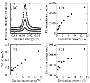
Figure 2: (a) Nanotube emission spectra at excitation powers of 0.47 $\mu$W (circles), 2.32 $\mu$W (squares), and 13.7 $\mu$W (triangles). Data are taken at an excitation energy of 1.553 eV. Data are offset for clarity and lines are Lorentzian fits to data. The same nanotube as in Fig. 1(b–e) is used. (b), (c), and (d) show photoluminescence intensity, full-width at half-maximum (FWHM) of the emission line, and emission energy as a function of excitation power, respectively.

We numerically solve this equation to obtain the exciton density profile, and the results for $L=0.3$ $\mu$m are plotted in Fig. 3(a). For $l$ shorter or comparable to $L$, the exciton density profile is nearly parabolic, indicating that majority of excitons diffuse to the unsuspended regions before recombining. Since the nonradiative recombination within unsuspended region efficiently removes excitons, the density of excitons stays low compared to longer nanotubes. As the nanotube length gets longer, the exciton density increases until it saturates when the nanotube length becomes long enough compared to $2(\sigma+L)$. In such a situation, most of the excitons recombine before they diffuse out to the unsuspended part, so that $l$ does not play a role.

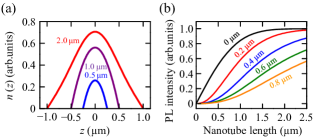
Figure 3: (a) Simulated exciton density spatial profile for $l=0.5$ $\mu$m (blue), 1.0 $\mu$m (purple), and 2.0 $\mu$m (red). Exciton diffusion length $L=0.3$ $\mu$m is used for obtaining these curves. (b) Simulated PL intensity as a function of $l$ for $L=0.0$ $\mu$m (black), 0.2 $\mu$m (red), 0.4 $\mu$m (blue), 0.6 $\mu$m (green), and 0.8 $\mu$m (orange).

In order to compute how the PL intensity changes with $l$, we integrate the exciton density profile to obtain the total number of excitons. We simulate the PL intensity for a range of nanotube length and a series of diffusion lengths, and plot them in Fig. 3(b). If the diffusion length is very short, the saturation of the PL intensity is expected for nanotube length longer than the laser spot size. As the diffusion length gets longer, the transition to the linear behavior shifts to longer nanotube length, and saturation would not be observed.

Now we compare the $l$ dependence of the measured PL intensity to the simulation [Fig. 4(a–c)]. We perform least square fits to the experimental data by looking for optimum values for $L$ and $N$. At all excitation powers, we find reasonable agreement between the data and the simulation. Although the experimental data show some dispersion from the fit, it is expected that there are some tube-to-tube variations in the PL intensity. Such inhomogeneities have been observed in PL imaging of very long SWCNTs Lefebvre:2006 , and can result from changes in the exciton lifetime $\tau$ induced by gas adsorption, contamination, or defects. We have computed such an effect, and found that our data falls into the band between the simulation results with lifetime set to $\pm 20$ % of the best fit. Taking such uncertainties in $\tau$ as the error in the determination of $L$, we plot the dependence of the diffusion length as a function of $P$ in Fig. 4(d).

The apparent diffusion length decreases with increasing $P$, which can be qualitatively explained by a reduction of $\tau$ caused by exciton-exciton annihilation. However, the $z$ and $l$ dependences of $\tau$ is not accounted for in our simple model, so it may not be accurate at high excitation powers. A more rigorous modeling is required to clarify the effects of exciton-exciton annihilation on $L$. Nevertheless, such effects should be small at lower powers. We find $L=610$ nm for the lowest $P$, and an extrapolation of the data down to $P=0$ $\mu$W suggests even longer $L$. The observed diffusion length is much longer compared to micelle-encapsulated SWCNTs Luer:2009 ; Cognet:2007 ; Georgi:2009 . It is possible that surfactants cause additional exciton scattering, and sonication may introduce defects in those samples.

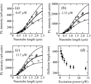
Figure 4: (a), (b), and (c) show measured photoluminescence intensity as a function of nanotube length for $P=0.47$ $\mu$W, 2.32 $\mu$W, and 13.7 $\mu$W, respectively. Polarization dependence of the detection efficiency has been corrected. The thick solid lines represent the best fits and the thin lines correspond to simulation results with exciton lifetime scaled by $\pm 20$ % while all the other parameters were fixed. The best fits give $L=610$ nm, 430 nm, and 280 nm for (a), (b), and(c), respectively. (d) Excitation power dependence of exciton diffusion length.

The diffusion length can give us some insight to transport properties of excitons. From $L=610$ nm, we obtain $D=44$ cm² s^-1 for $\tau=85$ ps Xiao:2010 . Using the Einstein relation $\mu kT=eD$, where $\mu$ is the exciton mobility, $k$ is the Boltzmann constant, and $e$ is the electronic charge, we find $\mu=1.7\times 10^{3}$ cm² V^-1 s^-1. This is comparable to reported values of carrier mobilities in SWCNTs Javey:2002 ; Durkop:2004 ; Zhou:2005 , although different scattering mechanisms and effective masses should be considered in general.

In summary, the diffusion length of excitons in air-suspended $(9,8)$ SWCNTs has been measured to be as long as 610 nm. At higher excitation powers, the apparent diffusion length becomes shorter due to exciton-exciton annihilation. Long diffusion lengths are favorable for fabricating single photon sources from SWCNTs Hogele:2008 , because such a device will need to have a length less than the exciton diffusion length to ensure annihilation of excess excitons.

- (1) P. Avouris, M. Freitag, and V. Perebeinos, Nature Photon. 2, 341 (2008).
- (2) F. Wang, G. Dukovic, L. E. Brus, T. F. Heinz, Science 308, 838 (2005).
- (3) Y. Murakami and J. Kono, Phys. Rev. B 80, 035432 (2009).
- (4) Y.-F. Xiao, T. Q. Nhan, M. W. B. Wilson, and J. M Fraser, Phys. Rev. Lett. 104, 017401 (2010).
- (5) F. Wang, G. Dukovic, E. Knoesel, L. E. Brus, and T. F. Heinz, Phys. Rev. B 70, 241403(R) (2004).
- (6) Y.-Z. Ma, L. Valkunas, S. L. Dexheimer, S. M. Bachilo, and G. R. Fleming, Phys. Rev. Lett. 94, 157402 (2005).
- (7) K. Matsuda, T. Inoue, Y. Murakami, S. Maruyama, and Y. Kanemitsu, Phys. Rev. B 77, 033406 (2008).
- (8) R. M. Russo, E. J. Mele, C. L. Kane, I. V. Rubtsov, M. J. Therien, and D. E. Luzzi, Phys. Rev. B 74, 041405(R) (2006).
- (9) L. Lüer, S. Hoseinkhani, D. Polli, J. Crochet, T. Hertel, and G. Lanzani, Nature Phys. 5, 54 (2009).
- (10) L. Cognet, D. A. Tsyboulski, J.-D. R. Rocha, C. D. Doyle, J. M. Tour, and R. B. Weisman, Science 316, 1465 (2007).
- (11) C. Georgi, M. Böhmler, H. Qian, L. Novotny, and A. Hartschuh, Phys. Status Solidi B 246, 2683 (2009).
- (12) K. Yoshikawa, K. Matsuda, and Y. Kanemitsu, J. Phys. Chem. C (2010), in press.
- (13) S. Maruyama, R. Kojima, Y. Miyauchi, S. Chiashi, and M. Kohno, Chem. Phys. Lett. 360, 229 (2002).
- (14) J. Lefebvre, Y. Homma, and P. Finnie, Phys. Rev. Lett. 90, 217401 (2003).
- (15) D. Mann, Y. K. Kato, A. Kinkhabwala, E. Pop, J. Cao, X. Wang, L. Zhang, Q. Wang, J. Guo, and H. Dai, Nature Nanotech. 2, 33 (2007).
- (16) J. Cao, Q. Wang, and H. Dai, Nature Mater. 4, 745 (2005).
- (17) J. Lefebvre, J. M. Fraser, Y. Homma, and P. Finnie, Appl. Phys. A 78, 1107 (2004).
- (18) Y. Ohno, S. Iwasaki, Y. Murakami, S. Kishimoto, S. Maruyama, and T. Mizutani, Phys. Rev. B 73, 235427 (2006).
- (19) J. Lefebvre, P. Finnie, and Y. Homma, Phys. Rev. B 70, 045419 (2004).
- (20) K. Yoshikawa, R. Matsunaga, K. Matsuda, and Y. Kanemitsu, Appl. Phys. Lett. 94, 093109 (2009).
- (21) P. Finnie, Y. Homma, and J. Lefebvre, Phys. Rev. Lett. 94, 247401 (2005).
- (22) S. Chiashi, S. Watanabe, T. Hanashima, and Y. Homma, Nano Lett. 8, 3097 (2008).
- (23) J. Lefebvre, D. G. Austing, J. Bond, and P. Finnie, Nano Lett. 6, 1603 (2006).
- (24) A. Javey, H. Kim, M. Brink, Q. Wang, A. Ural, J. Guo, P. McIntyre, P. McEuen, M. Lundstrom, and H. Dai, Nature Mater. 1, 241 (2002).
- (25) T. Dürkop, S. A. Getty, E. Cobas, and M. S. Fuhrer, Nano Lett. 4, 35 (2004).
- (26) X. Zhou, J.-Y. Park, S. Huang, J. Liu, and P. L. McEuen, Phys. Rev. Lett. 95, 146805 (2005).
- (27) A. Högele, C. Galland, M. Winger, and A. Imamoğlu, Phys. Rev. Lett. 100, 217401 (2008).