Exclusive diffractive photoproduction of dileptons by timelike Compton scattering

Abstract

We derive the forward photoproduction amplitude for the diffractive $\gamma p\to l^{+}l^{-}p$ reaction in the momentum space. within the formalism of $k_{\perp}$- factorization. Predictions for the $\gamma p\to l^{+}l^{-}p$ reaction are given using unintegrated gluon distribution from the literature. We calculate the total cross section as a function of photon-proton center of mass energy and the invariant mass distribution of the lepton pair. We also discuss whether the production of timelike virtual photons can be approximated by continuing to the spacelike domain $q^{2}<0$. The present calculation provides an input for future predictions for exclusive hadroproduction in the $p\,p\to p\,\,l^{+}l^{-}p$ reaction.

I Introduction

Measuring absolutely normalized cross sections at the LHC is of great importance for the high-energy physics community. This requires having a well understood luminosity monitor. Following the pioneering work Budnev , the QED process $pp\to pl^{+}l^{-}p$ via photon–photon fusion is often discussed as a process which can be used for measuring the luminosity at the LHC T02 ; P97 ; KCS08 . It is therefore very important to estimate other non-QED contributions to exclusive $l^{+}l^{-}$ production. One possible source of dileptons is the exclusive production of vector mesons or $Z$–bosons (see e.g. SS07 ; RSS08 ; CSS09 ). The dilepton pairs originating from these processes however have invariant masses close to the mass of the decaying state. In Figure 1 we show an exclusive diffractive mechanism which produces continuum dilepton pairs, and hence may compete with the standard QED process. In this reaction the coupling of the photon to the proton is known and can be expressed in terms of the nucleon electromagnetic form factors. At the small transferred momenta ($t_{1}$ or $t_{2}$) of relevance, it is sufficient, in the high energy limit, to include the Dirac electromagnetic form factor. Besides its role as a possible background to electromagnetic lepton pair production, the $\gamma p\to\gamma^{*}p$ amplitude may contain interesting information on the small–$x$ gluon distribution in the nucleon.

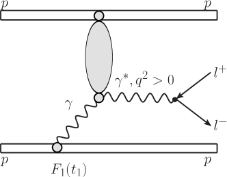
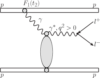
Figure 1: An example of the non-QED mechanism for the prodution of opposite charge leptons in the $pp\to ppl^{+}l^{-}$ reaction.

In the present work we shall concentrate on the photon-pomeron subprocess. In Fig.2 we show a QCD mechanism, where the photon splits into a quark-antiquark pair which interacts with the proton through the exchange of an off-diagonal QCD gluon ladder. In principle this process could have been studied at HERA. In Fig.2 the incoming photon is spacelike, (or quasireal) but the outgoing photon is timelike, i.e. its virtuality $q^{2}>0$. This process is often called timelike Compton scattering (TCS) in the literature, although the specific mechanism considered by us is maybe better termed a QCD version of (virtual) Delbrück scattering. A collinear factorisation treatment of timelike Compton scattering in terms of the nucleon’s skewed (mainly quark-) distributions can be found in Berger ; Belitsky . This approach is most relevant for lower center-of-mass energies. We will restrict ourselves to high energies, where the $t$-channel exchange is dominated by gluons, and choose a $k_{\perp}$–factorization formalism very similar to the one used in diffractive vector meson production I03 ; INS06 .

The TCS cross section has also been evaluated in a color-dipole model with a saturation-idea inspired dipole-nucleon cross section M08 . However there both incoming and outgoing photons were assumed to be spacelike. A recent estimate of high energy cross–sections in leading order collinear factorization, without explicit gluons, is found in PSW09 .

In this work we present the momentum–space formulation of timelike Compton scattering at small-$x$, taking due account of the timelike nature of the final state photon.

This paper is organized as follows. In the next section, we present the formalism which is used in our calculations. In Sec. III we present the main results for the $\gamma p\to l^{+}l^{-}p$ reaction. Finally, in the last section we summarize our results and show further perspectives.

II Formalism

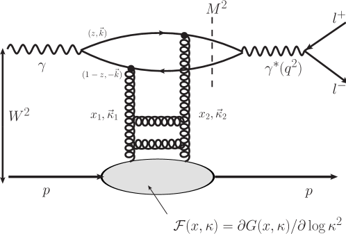
Figure 2: The diagram for the production of virtual timelike photons.

The photoproduction amplitude will be the major building block for our prediction of exclusive dilepton pair production. The amplitude for the reaction is shown schematically in Fig.2. In the diagram, we distinguish three stages of the process: first the incoming real photon fluctuates into a quark-antiquark pair, then a gluon ladder is exchanged between the $q\bar{q}$ pair and the proton and finally the $q\bar{q}$ pair recombines to form a virtual photon which subsequently decays into a lepton–antilepton pair.

The amplitude of the subprocess $\gamma p\to\gamma^{*}(q^{2})p$ is a sum of the contributions for a given flavour $f$ of quarks in the loop.

$${\cal M}(\gamma p\to\gamma^{*}(q^{2})p)=\sum\limits_{f}{\cal M}_{f}(\gamma p\to\gamma^{*}(q^{2})p).$$ (1)

Here the initial state photon is real, and hence transversely polarized. We take only the dominant $s$–channel helicity conserving contribution into account, and suppress helicities of photons/protons in our notation. The calculation of the amplitude follows the same procedure as for the exclusive production of vector mesons, which is explained in great detail in Ivanov’s thesis I03 . The main difference is that the final state light–cone wavefunction is replaced by a free quark propagator times the QED–spinor structure for the $q\bar{q}\to\gamma^{*}$ transition. The forward $\gamma p\to\gamma^{*}p$ amplitude for a given flavour contribution can then be written as:

$${\cal M}_{f}(\gamma p\to\gamma^{*}(q^{2})p)=W^{2}\,4\pi\alpha_{\mathrm{em}}\,e_{f}^{2}\,2\,\int_{0}^{1}dz\,\int_{0}^{\infty}\pi dk_{\bot}^{2}{{\cal A}_{f}(z,k_{\bot}^{2},W^{2})\over[k_{\bot}^{2}+m_{f}^{2}-z(1-z)q^{2}-i\varepsilon]}$$

$$=W^{2}\,4\pi\alpha_{\mathrm{em}}\,e_{f}^{2}\,2\,\cdot 2\,\int_{0}^{1/2}\frac{dz}{z(1-z)}\,\int_{0}^{\infty}\pi dk_{\bot}^{2}{{\cal A}_{f}(z,k_{\bot}^{2},W^{2})\over\left[{k_{\bot}^{2}+m_{f}^{2}\over z(1-z)}\,-q^{2}-i\varepsilon\right]},$$ (2)

where the explicit form of ${\cal A}_{f}(z,k_{\bot}^{2},W^{2})$ will be discussed below, $\alpha_{\mathrm{em}}$ is the QED fine–structure constant; $e_{f}=\frac{2}{3}$ for $u,c,t$ and $e_{f}=-\frac{1}{3}$ for $d,s,b$ is the quark charge. The transverse momentum squared of (anti-)quarks is denoted by $k^{2}$, their longitudinal momentum fractions are $z$ and $1-z$, respectively. The running coupling $\alpha_{s}$ enters at the scale $q^{2}={\mathrm{max}}\{\kappa^{2},k^{2}+m_{f}^{2}\}$, where $m_{f}$ is the quark mass for flavor $f$. Now notice, that the invariant mass of the $q\bar{q}$ pair is given by

$$M^{2}={k_{\bot}^{2}+m_{f}^{2}\over z(1-z)}\,,$$ (3)

so that the second line of Eq.(2) suggests a change of variables from $(z,k_{\bot}^{2})\to(M^{2},k_{\bot}^{2})$:

$${dz\,dk_{\bot}^{2}\over z(1-z)}\longrightarrow{dM^{2}\over M^{2}}\,{dk_{\bot}^{2}\over J}$$ (4)

Using the $z\leftrightarrow 1-z$ symmetry we could restrict ourselves to $0\leq z\leq 1/2$, so that from

$$z=z(M^{2},k_{\bot}^{2})={1\over 2}\left[1-\sqrt{1-4\frac{k_{\bot}^{2}+m_{f}^{2}}{M^{2}}}\,\right],$$ (5)

we obtain the jacobian factor

$$J=\sqrt{1-4\left(\frac{k_{\bot}^{2}+m^{2}}{M^{2}}\right)},$$ (6)

which introduces an integrable singularity (see e.g. Eq. 4). The integration domain is transformed as

$$\{0\leq z\leq 1/2\}\times\{0\leq k_{\bot}^{2}<\infty\}\longrightarrow\{4m_{f}^{2}\leq M^{2}<\infty\}\times\{0\leq k_{\bot}^{2}\leq(M^{2}-4m_{f}^{2})/4\}.$$ (7)

Finally, we can cast the amplitude in the form

$${\cal M}_{f}(\gamma p\to\gamma^{*}(q^{2})p)=W^{2}\,16\pi^{2}\alpha_{\mathrm{em}}e_{f}^{2}\ \cdot\int_{4m_{f}^{2}}^{\infty}\,{a_{f}(W^{2},M^{2})\over M^{2}-q^{2}-i\varepsilon}\,dM^{2}.$$ (8)

Here $a_{f}(W^{2},M^{2})$ is related to the diffractive amplitude for the $\gamma p\to q\bar{q}p$ transition Nikolaev:1991et , however with the spinorial contractions from the final state performed. For the lack of a better name we will refer to it as the spectral distribution or spectral density. Its imaginary part is given by the integral:

$$\Im m\,a_{f}(W^{2},M^{2}) = {1\over M^{2}}\int_{0}^{{1\over 4}M^{2}-m_{f}^{2}}\,\frac{dk_{\bot}^{2}}{J}\,\Im m\,{\cal A}_{f}(z(M^{2},k_{\bot}^{2}),k_{\bot}^{2},W^{2})\,.$$ (9)

with

$$\Im m{\cal A}_{f}(z,k_{\bot}^{2},W^{2}) =\pi\int_{0}^{\infty}{\pi d\kappa^{2}\over\kappa^{4}}\alpha_{s}(q^{2}){\cal F}(x_{\mathrm{eff}},\kappa^{2})\Big{[}A_{0f}(z,k_{\bot}^{2})\,W_{0f}(k_{\bot}^{2},\kappa^{2})$$ (10)

$$+A_{1f}(z,k_{\bot}^{2})\,W_{1f}(k_{\bot}^{2},\kappa^{2})\Big{]}\,,$$

where the auxiliary functions $A_{1,0f},W_{1,0f}$ can be taken from Ref. RSS08 :

$$A_{0f}(z,k_{\bot}^{2}) = m_{f}^{2},\,\,A_{1f}(z,k_{\bot}^{2})=[z^{2}+(1-z)^{2}]{k_{\bot}^{2}\over k_{\bot}^{2}+m_{f}^{2}},$$

$$W_{0f}(k_{\bot}^{2},\kappa^{2}) = {1\over{k_{\bot}^{2}+m_{f}^{2}}}-{1\over\sqrt{(k_{\bot}^{2}-m_{f}^{2}-\kappa^{2})^{2}+4m_{f}^{2}k_{\bot}^{2}}},$$

$$W_{1f}(k_{\bot}^{2},\kappa^{2}) = 1-{k_{\bot}^{2}+m_{f}^{2}\over 2k_{\bot}^{2}}\left(1+{k_{\bot}^{2}-m_{f}^{2}-\kappa^{2}\over\sqrt{(k_{\bot}^{2}-m_{f}^{2}-\kappa^{2})^{2}+4m_{f}^{2}k_{\bot}^{2}}}\right).$$ (11)

Given the relation to the diffractive $\gamma p\to q\bar{q}p$ amplitude we feel justified to obtain the real part from the standard derivative form of the dispersion relation:

$$\Re e\,{\cal A}_{f}(z,k_{\bot}^{2},W^{2})=\Im m{\cal A}_{f}(z,k_{\bot}^{2},W^{2})\cdot\tan\Big{(}{\pi\over 2}{\partial\log\Im m{\cal A}_{f}(z,k_{\bot}^{2},W^{2})\over\partial\log W^{2}}\Big{)}.$$ (12)

The function ${\cal F}(x,\kappa^{2})$ is the unintegrated gluon distribution of the proton, which at large values of gluon transverse momenta can be expressed in terms of the collinear gluon distribution as

$${\cal F}(x,\kappa^{2})={\partial G(x,\kappa^{2})\over\partial\log\kappa^{2}},$$ (13)

In the present analysis we use an unintegrated gluon distribution obtained by fitting to the structure function data measured at HERA IN02 . Following I03 ; INS06 , we correct for skewedness effects by taking the unintegrated at $x_{\mathrm{eff}}=c_{\mathrm{skewed}}\,{M^{2}\over W^{2}}$  with $c_{\mathrm{skewed}}=0.41$. To calculate the integral in Eq.(8) for $q^{2}>4m_{f}^{2}$ we use the Plemelj-Sokhocki formula:

$${1\over x-i\varepsilon}=\mathrm{PV}{1\over x}+i\pi\delta(x),$$ (14)

where $\mathrm{PV}$ denotes the principal value integral. We can finally represent real and imaginary part of the forward TCS amplitude as

$$\Im m{\cal M}_{f}(\gamma p\to\gamma^{*}(q^{2})p) =W^{2}\,16\pi^{2}\alpha_{\mathrm{em}}e_{f}^{2}\cdot\Big{\{}\theta(4m_{f}^{2}-q^{2})\,\int_{4m_{f}^{2}}^{\infty}\,dM^{2}{\Im m\,a_{f}(W^{2},M^{2})\over M^{2}-q^{2}}$$

$$+\theta(q^{2}-4m_{f}^{2})\,\Big{(}\mathrm{PV}\int_{4m_{f}^{2}}^{\infty}dM^{2}{\Im m\,a_{f}(W^{2},M^{2})\over M^{2}-q^{2}}\,+\pi\,\Re e\,a_{f}(W^{2},q^{2})\Big{)}\Big{\}},$$

$$\Re e{\cal M}_{f}(\gamma p\to\gamma^{*}(q^{2})p) =W^{2}\,16\pi^{2}\alpha_{\mathrm{em}}c_{f}^{2}\cdot\Big{\{}\theta(4m_{f}^{2}-q^{2})\,\int_{4m_{f}^{2}}^{\infty}\,dM^{2}{\Re e\,a_{f}(W^{2},M^{2})\over M^{2}-q^{2}}$$

$$+\theta(q^{2}-4m_{f}^{2})\,\Big{(}\mathrm{PV}\int_{4m_{f}^{2}}^{\infty}dM^{2}{\Re e\,a_{f}(W^{2},M^{2})\over M^{2}-q^{2}}\,-\pi\,\Im m\,a_{f}(W^{2},q^{2})\Big{)}\Big{\}}.$$

Two comments are in order on the final form of the TCS amplitude (LABEL:eq:final): firstly, the “$i\pi$”–terms from the decomposition (14) lead to a quite nontrivial structure of the amplitude in terms of the spectral distribution $a_{f}$. In particular, the TCS amplitude will not be a monotonous function of $q^{2}$. Secondly, we should remember that these “$i\pi$”–terms derive from the cut through the $q\bar{q}$ pair which exists in the perturbative amplitude, when $q^{2}>4m_{f}^{2}$. Clearly in the real hadronic world, there are no cuts due to quarks going on–shell, and our amplitude must, as usual, be interpreted in a parton–hadron duality sense.

As a last step we must extend our amplitude to finite momentum transfers. For simplicity we will assume it to have the following factorized form

$${\cal M}_{f}(\gamma p\to\gamma^{*}(q^{2})p;t)={\cal M}_{f}(\gamma p\to\gamma^{*}(q^{2})p)\,\exp[Bt]\,,$$ (16)

which should be sufficiently accurate for small $t$, within the diffraction cone. The total cross section for the $\gamma p\to\gamma^{*}p$ process can then be obtained as

$$\sigma(\gamma p\to\gamma^{*}(q^{2})p)={(\Re e{{\cal M}\over W^{2}})^{2}+(\Im m{{\cal M}\over W^{2}})^{2}\over 16\pi B},$$ (17)

where for a first estimation we shall take $B=4\,\mathrm{GeV}^{-2}$.

The invariant mass distribution of dileptons for the $\gamma p\to l^{+}l^{-}p$ reaction which can be accessed in experiment is given by:

$${d\sigma\over dq^{2}}(\gamma p\to l^{+}l^{-}p)={\alpha_{\mathrm{em}}\over 3\pi q^{2}}\cdot\sigma(\gamma p\to\gamma^{*}(q^{2})p),$$ (18)

where $l^{+}l^{-}$ means either $e^{+}e^{-}$ or $\mu^{+}\mu^{-}$. This simple formula applies only when $q^{2}\gg m_{l}^{2}$.

III Results

Here we present predictions for the $\gamma p\to l^{+}l^{-}p$ reaction. In Fig.3 we show spectral density as a function of $M^{2}$ (invariant mass of the $q\bar{q}$ pair) for different $\gamma p$ center of mass energies: $W=100,500,1000$ GeV and for $u,d,s,c$ quarks separately. The energy dependence of the spectral density derives from the $x_{\mathrm{eff}}$– dependence of the unintegrated gluon density. This is why we observe a growth of the spectral density with energy. For large invariant mass of the $q\bar{q}$ pair the spectral density tends to zero, which ensures the convergence of the integrals in (LABEL:eq:final).

Figure 3: Spectral density $(a_{f})$ for different flavours: solid line for u,d, dashed line for s, dotted line for c at W =100, 500, 1000 GeV. In the left row we show the imaginary part $\Im m\,a_{f}$, while in the right row, we show the real part $\Re e\,a_{f}$.

In Fig. 4 we show the invariant mass distribution $d\sigma/dq^{2}$ of dileptons in the $\gamma p\to l^{+}l^{-}p$ reaction as a function of photon-proton center-of-mass energy at fixed values of the invariant masses of the dilepton pairs ( $q^{2}$). Here all flavours are included in the amplitude. In general, the higher invariant mass, the faster growth with the photon-proton energy. This points to the fact that the unintegrated glue is probed at on average harder scales, where it has a faster $x$–dependence.

Figure 4: The cross section for $\gamma p\to l^{+}l^{-}p$ as a function of center-of-mass photon-proton energy for fixed values of the dilepton invariant mass.

Figure 5: ${\sigma}_{tot}(\gamma p\to l^{+}l^{-}p;q_{min}^{2})$ for $q_{min}^{2}=0.1,0.5,1.0,1.5\,GeV^{2}$.

In Fig. 5 we show cross section integrated over dilepton invariant mass

$${\sigma}_{tot}(\gamma p\to l^{+}l^{-}p;q_{min}^{2})=\int_{q_{min}^{2}}^{\infty}{d\sigma\over dq^{2}}dq^{2}\,.$$ (19)

These cross sections are by a factor of about 5 larger than those in M08 .

In Fig.6 we show the invariant mass distribution of dileptons $d\sigma/dq^{2}$ as a function of dilepton invariant mass $q^{2}$ at fixed values of $\gamma p$ energy. An interesting feature of the invariant mass distribution is a cusp at $q^{2}\sim 9\,{\mathrm{GeV}}^{2}$. Notice that this is the vicinity of $q^{2}\sim 4m_{c}^{2}$. Indeed the cusp is caused by the $c\bar{c}$ contribution to the amplitude which changes sign in this region. This is a unique feature of the structure of the amplitude (LABEL:eq:final) with timelike final state photons. Here one should however remember the caveat on the absence of quark thresholds, most optimistically one may hope that such a structure survives in the vicinity of $q^{2}\sim 4m_{D}^{2}$.

Figure 6: Distribution in $q^{2}$ for W = 100, 500, 1000 GeV.

Figure 7: The ratio of the cross section ${{d\sigma\over dq^{2}}timelike\over{d\sigma\over dq^{2}}spacelike}$ as a function of $q^{2}$.

Finally, it is interesting to investigate how well the dilepton mass spectrum can be calculated from the amplitude for production of spacelike photons in the final state. In this case one would replace Eq.(LABEL:eq:final) by the straightforward

$${\cal{M}}_{f}^{{\mathrm{spacelike}}}(\gamma p\to\gamma^{*}(q^{2})p)=W^{2}\,16\pi^{2}\alpha_{\mathrm{em}}e_{f}^{2}\cdot\int_{4m_{f}^{2}}^{\infty}\,{a_{f}(W^{2},M^{2})\over M^{2}+q^{2}}\,dM^{2}.$$ (20)

Notice that in distinction to the timelike case, this is a monotonous function of $q^{2}$. In Fig. 7 we show the ratio of $d\sigma/dq^{2}$ for the (correct) timelike photons and the spacelike prescription as a function of $q^{2}$ at various fixed energies. We observe that, as expected, the spacelike prescription does not reproduce the structure present in the timelike amplitude. At large $q^{2}$ it gives a fairly reasonable description of the $q^{2}$–dependence, but is not able to reproduce the correct timelike results. The cross section for timelike photons is bigger by a factor of 3-4 compared to the spacelike photon prescription.

IV Conclusions

We have derived the amplitude for the exclusive diffractive photoproduction of lepton pairs in the $k_{\perp}$-factorisation approach in the momentum space. We have discussed several details of the formalism as well as differences compared to the existing calculation in the literature which ignored the fact that the ”produced” photons are timelike.

We have calculated the cross sections as a function of photon-proton center of mass energy as well as a function of dilepton invariant mass. We have demonstrated how important is the inclusion of correct dynamics (timelike outgoing photons instead of spacelike outgoing photons). As a consequence the cross sections obtained here are significantly larger than those obtained in the literature. We furthermore observed an interesting structure in the invariant mass distribution of dileptons around $q^{2}\sim 9\,\mathrm{GeV}^{2}$.

The amplitude for the $\gamma p\to l^{+}l^{-}p$ is the main ingredient of the diffractive amplitude for the $pp\to l^{+}l^{-}pp$ process. In the case of hadroproduction of dileptons the diffractive mechanism constitutes a background to the purely electromagnetic (photon–photon fusion) production of dileptons. The latter process was sugested in the literature as a luminosity monitor the LHC studies. How important is this background for differential distributions in the four-body $pp\to l^{+}l^{-}pp$ reaction will be studied in detail elsewhere.

Acknowledments

We are indebted to Janusz Chwastowski and Krzysztof Piotrzkowski for an interesting discussion. This work was partially supported by the MNiSW grants: N N202 236937, N N202 249235 and N N202 191634.

References

• (1) V.M. Budnev, I.F. Ginzburg, G.V. Meledin and V.G. Serbo, Phys. Lett.  B 39 (1972) 526; Nucl. Phys.  B 63 (1973) 519.
• (2) A.G Shamov and V.I. Telnov, Nucl. Instr. and Meth. A 494 (2002) 51.
• (3) K. Piotrzkowski, Proposal for luminosity measurement at LHC. ATLAS note PHYS-96-077, 1996, unpublished. D. Bocian and K. Piotrzkowski, Acta Phys. Polon. B 35 (2004) 2417.
• (4) M.W. Krasny, J. Chwastowski, K. Słowikowski, Nucl. Instr. and Meth. A 584 (2008) 42-52.
• (5) W. Schäfer and A. Szczurek, Phys. Rev. D76 (2007) 094014.
• (6) A. Rybarska, W. Schäfer and A. Szczurek, Phys. Lett. B668,126 (2008).
• (7) A. Cisek, W. Schäfer and A. Szczurek, Phys. Rev. D80 (2009) 074013.
• (8) E.R. Berger, M. Diehl and B. Pire, Eur. Phys. J.  C 23 (2002) 675.
• (9) A.V. Belitsky and D. Mueller, Phys. Rev. Lett.  90 (2003) 022001.
• (10) I.P. Ivanov, [arXiv:hep-ph/0303053].
• (11) I.P. Ivanov, N.N. Nikolaev and A.A. Savin, Phys. Part. Nucl. 37:1-85,(2006).
• (12) M.V.T. Machado, Phys. Rev. D78 (2008) 034016.
• (13) B. Pire, L. Szymanowski and J. Wagner, Phys. Rev. D79 (2009) 014010.
• (14) N. Nikolaev and B.G. Zakharov, Z. Phys.  C 53 (1992) 331; Phys. Lett.  B 332 (1994) 177.
• (15) I.P. Ivanov and N.N. Nikolaev, Phys. Rev. D65 (2002) 054004.