Resonant scattering by realistic impurities in graphene

Abstract

We develop a first-principles theory of resonant impurities in graphene and show that a broad range of typical realistic impurities leads to the characteristic sublinear dependence of the conductivity on the carrier concentration. By means of density functional calculations various organic groups as well as ad-atoms like H absorbed to graphene are shown to create midgap states within $\pm 0.03$ eV around the neutrality point. A low energy tight-binding (TB) description is mapped out. Boltzmann transport theory as well as a numerically exact Kubo formula approach yield the conductivity of graphene contaminated with these realistic impurities in accordance with recent experiments.

The mechanism determining the charge carrier mobility of present graphene samples is being controversially debated. The main experimental fact requiring an explanation is that, away from the neutrality point, the conductivity of graphene is weakly temperature dependent and approximately proportional to the carrier concentration $n_{e}$ Novoselov et al. (2005); Zhang et al. (2005). This definitely requires the assumption of some long-range interactions with scattering centers. The Coulomb interaction with charge impurities is an “explanation by default” Cou . However, it seems that some experimental data cannot be explained in this way, especially, a relatively weak sensitivity of the electron mobility to dielectric screening Ponomarenko et al. (2009). Thus, alternative scattering mechanisms are also discussed, such as frozen ripples Katsnelson and Geim (2008) and resonant scatterers Ostrovsky et al. (2006); Katsnelson and Geim (2008); Katsnelson and Novoselov (2007); Stauber et al. (2007). In the first case the long-range character of the interactions is due to the long-range character of elastic deformations and in the second one due to divergence of the scattering length. New experimental data Ni et al. (2010) seem to support the latter possibility.

Theoretically, both suggestions face with serious problems. The “ripple” mechanism requires quenching of the thermal bending fluctuations Katsnelson and Geim (2008); Wehling et al. (2008a), but there are still no realistic scenarios of such a quenching. Resonant scattering naturally appears for vacancies Stauber et al. (2007) but they do not exist, in noticeable concentrations, in graphene samples if they are not created artificially, e.g., by irradiation Chen et al. (2009). Adsorbates on graphene can provide resonances (quasilocalized states) close enough to the neutrality point Wehling et al. (2007, 2008b); Wehling et al. (2009a, b) but not necessarily Wehling et al. (2007); Robinson et al. (2008). For impurity resonances some $100$ meV off the neutrality point the conductivity should display a pronounced electron-hole asymmetry Robinson et al. (2008) which is not observed in experiments. So, it is not clear whether resonant impurity scattering can be the main limiting factor in a general case.

In this Letter, we build a first-principles theory of electron scattering by realistic resonant impurities, such as various organic molecules which are always present in exfoliated graphene samples Meyer et al. (2007); Gass et al. (2008). Combining the Boltzmann equation approach and a numerically exact Kubo formula consideration with first-principles parameters, we show that this class of impurities can limit electron transport in typical exfoliated graphene samples and explain the experimentally observed concentration dependence of the conductivity.

Exfoliated graphene samples are contaminated with long polymer chains Meyer et al. (2007); Gass et al. (2008). Most important about these contaminants is their possibility to form a chemical bond to carbon atoms from the graphene sheet. To model such a situation we carry out density functional theory (DFT) calculations of graphene with adsorbed CH₃, C₂H₅, CH₂OH (as simplest examples of different organic groups), as well as H and OH groups. From the resulting supercell band structures we derive effective interaction parameters entering a TB model and find that the exact chemical composition is not essential: the parameters are very similar for all adsorbates except for the case of hydroxyl. This facilitates us to obtain the effect of the contamination on the electron conductivity.

An atomistic description of the graphene adsorbate systems is achieved by DFT calculations within the generalized gradient approximation (GGA) Perdew et al. (1992) on $3\times 3$-$9\times 9$ graphene supercells containing one impurity. Using the Vienna Ab Initio Simulation Package (VASP) Kresse and Hafner (1994) with the projector augmented wave (PAW) Blöchl (1994); Kresse and Joubert (1999) basis sets, we obtain fully relaxed adsorption geometries and calculate the supercell band structures.

The DFT results for CH₃, C₂H₅, CH₂OH on graphene are shown in Fig. 1a and compared to H and OH adsorbates. All of these impurities bind covalently to graphene and create a midgap state as characteristic for monovalent impurities Wehling et al. (2009b). For all adsorbates except OH the midgap state lies within $\pm 0.03$ eV around the neutrality point. As the supercell band structures for the organic groups and for H on graphene virtually coincide within an energy range of more than $\pm 1$ eV, it becomes clear that the parameters of the midgap state depend very weakly on the adsorbed group and, thus, can be considered as robust for further use in the transport theory.

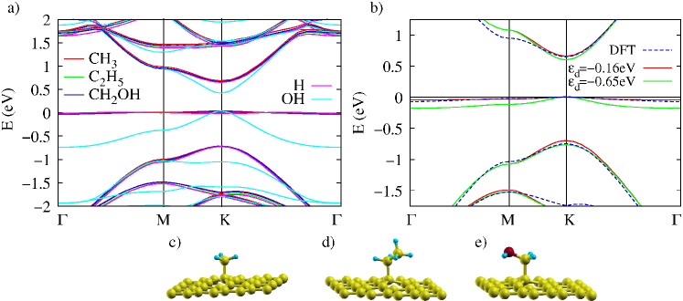
Figure 1: (Color online) (a) Band structures of $4\times 4$ graphene supercells with CH₃, C₂H₅, CH₂OH, H and OH adsorbates and the respective adsorption geometries of the CH₃, C₂H₅, CH₂OH (c-e) groups. (b) Comparison of the supercell band structure of graphene with CH₃ as obtained from DFT to the TB models with $V=2t$ and on-site energies $\epsilon_{d}=-0.16$ eV and $\epsilon_{d}=-0.65$ eV.

For an analytical description of these systems we start with a TB model of graphene,

$$\hat{H}=-t\sum_{<i,j>}c^{\dagger}_{i}c_{j},$$ (1)

where $c_{i}$ denotes the Fermi operator of an electron in the carbon $p_{z}$ orbital at site $i$, the sum includes all pairs of nearest-neighbor carbon atoms, and $t\approx 2.6$ eV is the nearest-neighbor hopping parameter. In this framework, we consider a “non-interacting Anderson impurity”, adding to the (1) the localized state, $\hat{H}_{\text{imp}}=\epsilon_{d}d^{\dagger}d,$ with on-site energy $\epsilon_{d}$ and corresponding Fermi operator $d$, which is coupled to the graphene bands by $\hat{V}=Vc^{\dagger}_{0}d+\rm{H.c.}$.

To describe electron transport in pristine as well as doped graphene correctly, the analytical model has to recover the realistic system within an energy window of some $100$ meV around the neutrality point. Applying the same supercell boundary conditions as in the DFT simulations to the TB impurity model, we obtain the TB supercell band structures as depicted in Fig. 1 b. The band structure of graphene with a methyl group is well fitted with $V\approx 2t=5.2$ eV and $\epsilon_{d}\approx-t/16=-0.16$ eV.

For the DFT band structures of all other neutral functional groups we find a good fit of TB with $|V|\gtrsim 2t$ and $|\epsilon_{d}|\lesssim 0.1t\approx 0.26$ eV. The hybridization strength $V$ being a factor 2 larger than $t$ is in accordance with the hybridization for hydrogen ad-atoms from Ref. Robinson et al. (2008) and appears very reasonable, as the impurity forms a $\sigma$-bond with the host atom underneath . The on-site energies $|\epsilon_{d}|$ obtained here are significantly smaller than the value $\epsilon_{d}=1.7$ eV used for H in Ref. Robinson et al. (2008) which will make our results for the transport properties qualitatively different. We note that the model parameters extracted here are converged w.r.t. the supercell size.

The scattering of electrons caused by resonant impurities is described by the $T$-matrix (for a review, see Ref. Wehling et al., 2009a) $T(E)=\frac{V^{2}}{E-\epsilon_{d}-V^{2}g_{0}(E)}$, where $g_{0}(E)\approx\frac{E}{D^{2}}\ln\left|\frac{E^{2}}{D^{2}-E^{2}}\right|-i\pi N_{0}(E)$, with $N_{0}(E)=\frac{|E|}{D^{2}}\cdot\Theta(D-|E|)$ and $D=\sqrt{\sqrt{3}\pi}t\approx 6$ eV, is the local Green function of pristine graphene. Correspondingly, $N_{0}(E)$ is the density of states (DOS) per spin and per carbon atom. The $T$-matrix exhibits a resonance at $E\left(1-\frac{V^{2}}{D^{2}}\ln\left|\frac{E^{2}}{D^{2}-E^{2}}\right|\right)-\epsilon_{d}=0$ which is the energy of the midgap state. The impurity model parameters obtained from DFT lead to resonances in an energy region of $\pm 0.03$ eV around the Dirac point, which proves consistency of our TB model with DFT.

In the Boltzmann equation approach, the $T$-matrix can be used to estimate the conductivity $\sigma$: $\sigma=(2e^{2}/h)v_{F}k_{F}\tau$, where $v_{F}$ is the Fermi velocity and $k_{F}$ is the Fermi wave vector. For a concentration of $n_{i}$ impurities per carbon atom, the scattering rate reads as Mahan (2000); Shon and Ando (1998); Robinson et al. (2008) $\tau^{-1}=(2\pi/\hbar)n_{i}|T(E_{F})|^{2}N_{0}(E_{F})$ and yields the conductivity

$$\sigma \approx (2e^{2}/h)(2\pi n_{i}|T(E_{F})/D|^{2})^{-1}.$$ (2)

In the limit of resonant impurities with $V\to\infty$, we obtain $T\rightarrow-1/g_{0}(E)\approx-\left[\frac{2E}{D^{2}}\ln\left|\frac{E}{D}\right|\right]^{-1}$ for $E\ll D$. Hence, the conductivity reads in this limit as

$$\sigma \approx (2e^{2}/h)\frac{2}{\pi}\frac{n_{e}}{n_{i}}\ln^{2}\left|\frac{E_{F}}{D}\right|,$$ (3)

where $n_{e}=E_{F}^{2}/D^{2}$ is the number of charge carriers per carbon atom. Eq. (3) yields the same behavior as for vacancies Stauber et al. (2007). In the case of the resonance shifted with respect to the neutrality point the consideration of Ref. Katsnelson and Novoselov (2007) leads to the dependence

$$\sigma\propto\left(q_{0}\pm k_{F}\ln{k_{F}R}\right)^{2},$$ (4)

where $\pm$ corresponds to electron and hole doping, respectively, and $R$ is the effective impurity radius.

We now investigate to which extend realistic resonant impurities create sublinear behavior similar to Eqs. (3-4). To this end, we first estimate the conductivity according to Eq. (2) for different types of impurities (Fig. 2).

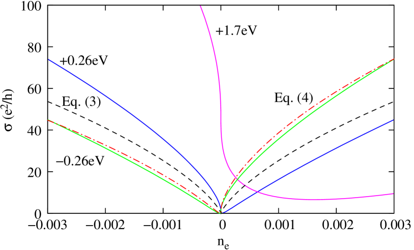
Figure 2: (Color online) Conductivity $\sigma$ in the Boltzmann approach as function of charge carrier concentration $n_{e}$ (in units of electrons per atom) for different impurities: Impurities with hybridization $V=2t=5.2$ eV and on-site energies $\epsilon_{d}=-0.26$, $0.26$, and $1.7$ eV in concentration $n_{i}=0.1\%$. (Curves are labelled by the corresponding $\epsilon_{d}$.) Fits to the $V\to\infty$ limit of Eq. (3) with $n_{i}=0.06\%$ (dashed) as well as Eq. (4) with $q_{0}=0.02\,\text{\AA}^{-1}$ (dash dotted) are shown. (Here, $n_{e}=E_{F}^{2}/D^{2}$ corresponds to the clean graphene DOS.)

For the resonant scatterers from Fig. 1 (except for OH) the conductivity curves are expected to lie within the region bounded by the curves belonging to $\epsilon_{d}=-0.26$ eV and $\epsilon_{d}=0.26$ eV. These curves are very similar to V-shape experimental curves Novoselov et al. (2005); Zhang et al. (2005); Ponomarenko et al. (2009); Ni et al. (2010) and can be roughly fitted to the limit of Eqs. (3) and (4). The effective radius $R$ resulting from Eq. (3) is $R=D/{\hbar v_{F}}\approx 0.9\text{\AA}$ and has been also used in the fit according to Eq. (4) in Fig. 2. Experimentally, sublinear behavior similar to Eqs. (3-4) has been observed Chen et al. (2009); Ni et al. (2010) with effective impurity radii in the range of $R=2.3-2.9\text{\AA}$. However, any estimation of effective radii should be considered only qualitatively, as $D$ and $R$ enter the conductivity logarithmically and a wide range of cut-offs lead to similar conductivity curves.

The result for impurities with $V=2t$ and $\epsilon_{d}=1.7$ eV, which corresponds to H ad-atoms in the model of Ref. Robinson et al. (2008), differs qualitatively from our results and from experimental data which emphasizes the crucial importance of a careful first-principles determination of the model parameters. In our model and for the charge carrier concentration being varied within $|n_{e}|<0.003$/C-atom$=1.1\cdot 10^{13}$ cm^-2, impurities like CH₃, C₂H₅, CH₂OH, or H attached to graphene lead to a Boltzmann conductivity with one distinct minimum close to the neutrality point.

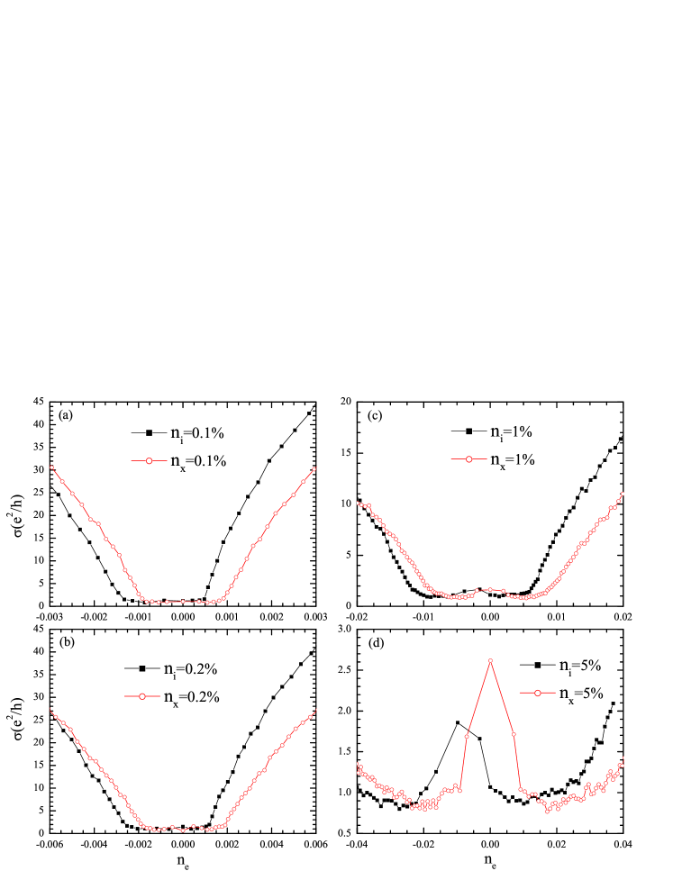
Figure 3: (Color online) Conductivity $\sigma$ as a function of charge carrier concentration $n_{e}$ (in units of electrons per atom) for different resonant impurity ($\varepsilon_{d}=-t/16,$ $V=2t$) or vacancy concentrations ($n_{x}$) : (a) $n_{i}=n_{x}=0.1\%,$ (b) $0.2\%,$ (c) $1\%,$ (d) $5\%$. Periodic boundary conditions are used with a sample containing (a) $8192\times 8192$ and (b-d) $4096\times 4096$ carbon atoms. The carrier concentrations $n_{e}$ are obtained from the integral of the corresponding DOS depicted in Fig. (4).

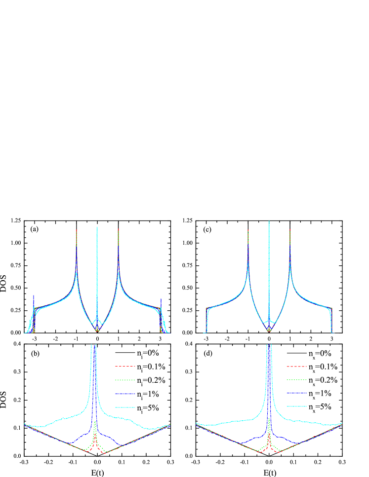
Figure 4: (Color online) Density of states as a function of energy $E$ for different resonant impurity ($\varepsilon_{d}=-t/16,$ $V=2t$) or vacancy concentrations: $n_{i}(n_{x})=0.1\%,$ $0.2\%,$ $1\%,$ $5\%$.

At low charge carrier concentrations or high impurity concentrations, the Boltzmann approach becomes questionable. To understand the on-set of this parameter regime and the behavior of the conductivity in this regime, we performed numerically exact calculations of the conductivity in the TB model (1) using the Kubo formula. [See kub .] The results for two types of resonant scatterers, adsorbed atoms with $\epsilon_{d}=-t/16$, $V=2t$ resembling CH₃ groups, and for vacancies are shown in Fig. 3. One can see that the Boltzmann equation is applicable only for impurity concentrations smaller than a few percent per site (already for 5% the difference in concentration dependence is essential). The Boltzmann approach does not work near the neutrality point where quantum corrections are dominant Ostrovsky et al. (2006); Katsnelson (2006); Auslender and Katsnelson (2007). In the range of concentrations, where the Boltzmann approach is applicable the conductivity as a function of energy fits very well the dependence of Eq. (4), with $q_{0}=0.02\text{\AA}^{-1}$, $R=0.6\text{\AA}$ for $n_{i}=0.1\%$, and $q_{0}=0$, $R=0.5\text{\AA}$ for $n_{x}=0.1\%$ with $k_{F}=E_{F}/(\hbar v_{F})$ as in clean graphene.

Close to the neutrality point the conductivity deviates from the Boltzmann equation result of Eq. (2). Boltzmann theory is not capable of yielding $\sigma=4e^{2}/\pi h$ for clean graphene at the neutrality point Ostrovsky et al. (2006); Katsnelson (2006). Moreover, resonant impurities lead to the formation of a low energy impurity band (see increased DOS at low energies in Fig. 4). At impurity concentrations on the order of a few percent (Fig. 3 c,d) this impurity band contributes to the conductivity and can lead to a maximum of $\sigma$ in the midgap region. Moreover, the impurity band can host two electrons per impurity. For impurity concentrations below $\sim 5\%$, this leads to a plateau shaped minimum of width $2n_{i}$ (or $2n_{x}$) in the conductivity vs. $n_{e}$ curves around the neutrality point. Analyzing the plateau width in experimental data (similar to the analysis for N₂O₄ acceptor states in Ref. Wehling et al., 2008b) can, thus, yield an independent estimate of impurity concentrations. For chiral disorder Altland (2002); Titov et al. (2010) corresponding to the resonant impurities considered, here, as well as short range disorder Lherbier et al. (2008a, b) (anti)localization effects can become important in cases like graphane, where impurity concentrations are varied between a few percent and $100\%$. In clean micron size samples with realistic impurity concentrations on the order of $n_{i}=0.01\%-0.1\%$ these effects present merely corrections: Upon doubling the simulation cell length ($4096\times 4096\,\to\,8192\times 8192$) at $n_{i}=0.1\%$ the changes of the conductivity at the neutrality point are below $10\%$.

Electron scattering in bilayer graphene has been proven to differ essentially from the single layer case in Ref. Katsnelson, 2007: For a scattering potential with radius much smaller than the de Broglie wavelength of electrons, the phase shift of $s$-wave scattering $\delta_{0}$ tends to a constant as $k\to 0$. Therefore, within the limit of applicability of the Boltzmann equation, the conductivity of a bilayer should be just linear in $n_{e}$, instead of sublinear dependence (4) for the single layer. The difference is that in the single layer, due to vanishing DOS at the Dirac point, the scattering disappears at small wave vectors as $\delta_{0}(k)\propto\frac{1}{\ln{kR}}$ (with $\ln^{2}{kR}$ on the order of 10 for typical amounts of doping) for resonant and as $\delta_{0}(k)\propto kR$ for the nonresonant impurities. Contrary, in the bilayer there are no restrictions on the strength of the scattering and even the unitary limit ($\delta_{0}=\pi/2$) can be reached at $k=0$. As follows from Ref. Katsnelson, 2007, a cylindric potential well of radius $R$, leads to $\delta_{0}=\pi/2$ if $\frac{d}{dR}\frac{J_{0}(qR)}{I_{0}(qR)}=0$, where $q$ is the wave vector inside the well, $J_{0}$ and $I_{0}$ are the Bessel functions of real and imaginary arguments, respectively. Thus, an assumption that resonant scattering is the main limiting factor for electron mobility in exfoliated graphene leads to the prediction that the dependence of $\sigma(n_{e})$ should be essentially different for the cases of bilayer and single layer, that is, linear and sublinear, respectively. This agrees with the experimental results Morozov et al. (2008).

In summary, we have demonstrated that realistic impurities in graphene frequently cause quasilocal peaks nearby the neutrality point. In particular, for various organic groups the formation of a carbon-carbon bond results in the appearance of midgap (resonant) states within $\pm 0.03$ eV around the neutrality point. They can be described as Anderson impurities with the hybridization parameter of about 2$t$ and on-site energies on the order of $|\epsilon_{d}|<t/10$. The resonant scattering model with these parameters describes satisfactory experimental data on the concentration dependence of charge carrier mobility for graphene.

We thank L. Oroszlány and H. Schomerus for discussions of Ref. Robinson et al., 2008. Support from SFB 668 (Germany), the Cluster of Excellence ”Nanospintronics” (LExI Hamburg), FOM (The Netherlands) and computer time at HLRN (Germany) and NCF (The Netherlands) are acknowledged.

References

- Novoselov et al. (2005) K. S. Novoselov et al., Nature 438, 197 (2005).
- Zhang et al. (2005) Y. Zhang et al., Nature 438, 201 (2005).
- (3) K. Nomura and A. H. Mac Donald, Phys. Rev. Lett. 96, 256602 (2006); T. Ando, J. Phys. Soc. Japan 75, 074716 (2006); S. Adam et al., Proc. Natl. Acad. Sci. USA 104, 18392 (2007); C. Jang et al., Phys. Rev. Lett. 101, 146805 (2008).
- Ponomarenko et al. (2009) L. A. Ponomarenko et al., Phys. Rev. Lett. 102, 206603 (2009).
- Katsnelson and Geim (2008) M. I. Katsnelson and A. K. Geim, Phil. Trans. R. Soc. A 366, 195 (2008).
- Ostrovsky et al. (2006) P. M. Ostrovsky, I. V. Gornyi, and A. D. Mirlin, Phys. Rev. B 74, 235443 (2006).
- Katsnelson and Novoselov (2007) M. I. Katsnelson and K. S. Novoselov, Solid State Commun. 143, 3 (2007).
- Stauber et al. (2007) T. Stauber, N. M. R. Peres, and F. Guinea, Phys. Rev. B 76, 205423 (2007).
- Ni et al. (2010) Z. H. Ni et al. (2010), eprint arXiv:1003.0202.
- Wehling et al. (2008a) T. O. Wehling et al., Europhys. Lett. 84, 17003 (2008a).
- Chen et al. (2009) J.-H. Chen et al., Phys. Rev. Lett. 102, 236805 (2009).
- Wehling et al. (2007) T. O. Wehling et al., Phys. Rev. B 75, 125425 (2007).
- Wehling et al. (2008b) T. O. Wehling et al., Nano Letters 8, 173 (2008b).
- Wehling et al. (2009a) T. O. Wehling, M. I. Katsnelson, and A. I. Lichtenstein, Chem. Phys. Lett. 476, 125 (2009a).
- Wehling et al. (2009b) T. O. Wehling, M. I. Katsnelson, and A. I. Lichtenstein, Phys. Rev. B 80, 085428 (2009b).
- Robinson et al. (2008) J. P. Robinson et al., Phys. Rev. Lett. 101, 196803 (2008).
- Meyer et al. (2007) J. C. Meyer et al., Nature 446, 60 (2007).
- Gass et al. (2008) M. H. Gass et al., Nature Nanotech. 3, 676 (2008).
- Perdew et al. (1992) J. P. Perdew et al., Phys. Rev. B 46, 6671 (1992).
- Kresse and Hafner (1994) G. Kresse and J. Hafner, J. Phys.: Condes. Matter 6, 8245 (1994).
- Blöchl (1994) P. E. Blöchl, Phys. Rev. B 50, 17953 (1994).
- Kresse and Joubert (1999) G. Kresse and D. Joubert, Phys. Rev. B 59, 1758 (1999).
- Mahan (2000) G. D. Mahan, Many-Particle Physics (Kluwer Academic/Plenum Publishers, 2000), 3rd ed.
- Shon and Ando (1998) N. H. Shon and T. Ando, J. Phys. Soc. Jpn. 67, 2421 (1998).
- (25) See suppl. material at http://link.aps.org/supplemental/ 10.1103/PhysRevLett.105.056802 and arXiv:1007.3930 for details of the Kubo formula approach.
- Katsnelson (2006) M. I. Katsnelson, Eur. Phys. J. B 51, 157 (2006).
- Auslender and Katsnelson (2007) M. Auslender and M. I. Katsnelson, Phys. Rev. B 76, 235425 (2007).
- Altland (2002) A. Altland, Phys. Rev. B 65, 104525 (2002).
- Titov et al. (2010) M. Titov et al., Phys. Rev. Lett. 104, 076802 (2010).
- Lherbier et al. (2008a) A. Lherbier et al., Phys. Rev. Lett. 100, 036803 (2008a).
- Lherbier et al. (2008b) A. Lherbier et al., Phys. Rev. Lett. 101, 036808 (2008b).
- Katsnelson (2007) M. I. Katsnelson, Phys. Rev. B 76, 073411 (2007).
- Morozov et al. (2008) S. V. Morozov et al., Phys. Rev. Lett. 100, 016602 (2008).