Optomechanics with molecules in a strongly pumped ring cavity

Abstract

Cavity cooling of an atom works best on a cyclic optical transition in the strong coupling regime near resonance, where small cavity photon numbers suffice for trapping and cooling. Due to the absence of closed transitions a straightforward application to molecules fails: optical pumping can lead the particle into uncoupled states. An alternative operation in the far off-resonant regime generates only very slow cooling due to the reduced field-molecule coupling. We predict to overcome this by using a strongly driven ring-cavity operated in the sideband cooling regime. As in the optomechanical setups one takes advantage of a collectively enhanced field-molecule coupling strength using a large photon number. A linearized analytical treatment confirmed by full numerical quantum simulations predicts fast cooling despite the off-resonant small single molecule - single photon coupling. Even ground state cooling can be obtained by tuning the cavity field close to the Anti-stokes sideband for sufficiently high trapping frequency. Numerical simulations show quantum jumps of the molecules between the lowest two trapping levels, which can be be directly and continuously monitored via scattered light intensity detection.

I Introduction

In recent years cavity cooling and manipulation of small polarizable particles has developed into an extended field of research cavcoolrev ; Lev-prospects-08 . Considerable theoretical progress understanding the strongly coupled atom-field dynamics including particle motion has been made in the past decades ritsch97 ; Morigi2007a ; deachapunya-slow-07 ; salzburger2009collective , and has been accompanied by impressive experimental achievements murr2006three ; zhang2009experimental ; leibrandt2009cavity ; slama2007superradiant ; hemmerich06 ; brennecke2008cavity .

As recently discussed in a detailed review article Lev-prospects-08 , a generalization to molecule cooling is limited by the inability of achieving sufficiently strong dispersive coupling to the cavity field. At the usable frequencies far from any internal molecular resonance the ratio of polarizability and mass is orders of magnitude below the value close to resonance. Although cooling persists in principle it slows down too much to be useful. One way out of this dilemma is the use of collective enhancement using a high density of particles inside the mode volume salzburger2009collective . Again in principle the mechanism has been shown to work for pre-cooled atoms chan2003observation , but it turns out to be technically challenging to implement the required high pressure and low temperature beam sources for molecules deachapunya-slow-07 .

As an alternative route one can instead take a clue from the field of optomechanics, where motional degrees of freedom of large vibrating objects such as micro-mirrors Groeblacher-demonstration-09 , toroidal microresonators wall vibrations Schliesser-resolved-09 , nano-membranes thompson-strong-08 , levitated nanospheres chang-cavity-09 or even viruses isart-towards-09 are manipulated via radiation pressure coupling to a light field. Such systems not only exploit directed collective scattering (reflection) from a large number of very weak scatterers but in addition rely on generating a stronger light force just by applying very high light intensities. As the effective mechanical coupling grows with the intracavity field amplitude (i.e. the square root of the photon number), the inherently small single photon coupling rate, proportional to the extent of the objects zero-point-motion, can be augmented by several orders of magnitude to produce strong friction forces.

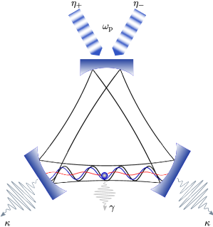
Figure 1: A ring cavity with two degenerate modes (cosine: black line and sine: red line) with the same wave vector $k$. The cosine mode is strongly pumped and is responsible for trapping a polarizable particle around one of its intensity minima. Depicted in the figure is also the effective potential seen by the particle (blue line) as it is shifted around depending on the dynamical occupancy of the sine mode.

In this work we consider the corresponding limit for a weakly polarizable particle (molecule) in a ring cavity. In a previous analysis concentrating in the low photon number but strong atom-field coupling limit the ring cavity geometry has been shown to lead to enhanced cooling of atoms by only a factor two at best gangl-cold-00 ; murr-large-06 . Let us instead focus on the high-field limit for a symmetrically pumped ring cavity as in typical optomechanical systems to study the corresponding coupling enhancement for a very weakly coupled molecule (see Fig. 1). For symmetric pumping it proves useful to decompose the ring cavity field in a cosine and sine mode instead of the more common propagating mode expansion. In this basis photons from the highly excited driven cosine mode are scattered into the almost empty sine mode. Amplitude and phase of this weak single molecule light scattering to the sine mode is highly spatially dependent and strongly enhanced by the presence of a large field amplitude in the cosine mode. The situation for a high field seeking particle is illustrated in Fig. 1. The particle is trapped close to the antinodes of the highly populated cosine mode, while the $\pi/2$-shifted sine mode provides the weakly–populated quantum mode that produces sideband cooling. Actually an analogous situation will occur for any cavity geometry with two almost degenerate modes with differing mode functions.

In the following using different theoretical approaches we will demonstrate two central physical effects for such a setup: i) the efficiency of cooling in the dynamical regime is considerably improved over cooling in a typical standing wave cavity with large circulating power and ii) for particles trapped in a standing wave cosine mode in a ring cavity the coupling of the single molecule to the corresponding sine mode is equivalent to an optomechanical coupling with a coupling strength enhanced by a power of the intracavity cosine mode photon number.

The paper is structured as follows: in Sec. II we present an effective quantum Langevin description for the coupled dynamics of a polarizable particle moving in the field of a ring cavity. In Sec. III we ignore noise terms and study important dynamical features of the underlying classical dynamics and compare this to the typical standing wave cavity cooling. In Sec. IV we concentrate on the case of an intense pump field with strongly confined particle motion, where the dominant interaction couples the sine mode to the particle motion. In Sec. V we numerically study the cooling process using wave function simulations and we present numerical examples for quantum trajectories exhibiting the evolution of the molecule’s state under continuous monitoring of the scattered field. Sec. VI contains more detailed discussions on the physical interpretation of the cooling mechanism in this setup. Conclusions are presented in the closing Sec. VII.

II Quantum Langevin approach to ring cavity cooling

We consider a one-dimensional configuration as illustrated in Fig. 1, where a polarizable particle of mass $m$ modeled as a two-level system with energy splitting $\hbar\omega_{a}$ is off-resonantly coupled to the field in a ring cavity. For a wave vector $k$ (corresponding frequency $\omega_{c}$) there are two degenerate counter-propagating modes of the cavity driven with amplitudes $\eta_{+}=\eta_{-}=\eta$. One can rethink this in terms of cosine and sine standing wave modes, with the cosine mode driven with $\eta$ while the sine mode is unpumped. The two optical modes are represented by field operators $a_{c}$ (cosine mode), with commutator $\left[a_{c},a_{c}^{\dagger}\right]=1$ and $a$ (sine mode) with $\left[a,a^{\dagger}\right]=1$. The cosine mode is driven by a laser at frequency $\omega_{p}$ and amplitude $\eta$ with detuning $\Delta=\omega_{p}-\omega_{c}$. Both fields decay at rate $2\kappa$ through the mirrors. The particle’s quantized position and momentum operators are $\hat{x}$ and $\hat{p}$, $\left[\hat{x},\hat{p}\right]=i\hbar$. The field, strongly detuned from the particle’s resonance by $\Delta_{a}=\omega_{a}-\omega_{p}$, is coupled with strength $g$ so that we have very low saturation and the spontaneous emission $\gamma$ plays only a minor role, as discussed in more detail later in Sec. VI. The position dependent intracavity intensity seen by a particle at position $\hat{x}$ can be written as $(a_{c}^{\dagger}\cos k\hat{x}+a_{s}^{\dagger}\sin k\hat{x})(a_{c}\cos k\hat{x}+a_{s}\sin k\hat{x})$. Elimination of the internal degrees of freedom of the particle in the limit of very large detuning $\Delta_{a}\gg\gamma$ leads to an effective position modulated energy shift gangl-cold-00

$$U(\hat{x})=a_{c}^{\dagger}a_{c}U_{c}\left(\hat{x}\right)+a_{s}^{\dagger}a_{s}U_{s}(\hat{x})+\left(a_{c}^{\dagger}a_{s}+a_{c}a_{s}^{\dagger}\right)U_{cs}(\hat{x}),$$

where $U_{c}\left(\hat{x}\right)=U_{0}\cos^{2}k\hat{x}$, $U_{s}\left(\hat{x}\right)=U_{0}\sin^{2}k\hat{x}$,$U_{cs}(\hat{x})=U_{0}\sin k\hat{x}\cos k\hat{x}$ and $U_{0}\simeq g^{2}/\Delta_{a}$. We arrive at an effective master equation for the system:

$$\dot{\rho}=-\frac{i}{\hbar}\left[H,\rho\right]+L_{c}\rho+L\rho,$$ (1)

where the Hamiltonian evolution is governed by

$$H=\frac{\hat{p}^{2}}{2m}-\hbar\Delta\left(a_{c}^{\dagger}a_{c}+a_{s}^{\dagger}a_{s}\right)-\hbar U(\hat{x})+i\hbar\left(\eta a_{c}^{\dagger}-\eta^{\ast}a_{c}\right),$$ (2)

and the Liouvilian describes dissipation via cavity decay $L_{c}\rho=\kappa D\left[a_{c}\right]\rho$ and $L\rho=\kappa D\left[a\right]\rho$, where the superoperator’s $D$ action on a generic operator $c$ is defined as $D\left[c\right]=2c\rho c^{\dagger}-c^{\dagger}c\rho-\rho c^{\dagger}c$. Notice that we have ignored spontaneous emission in the Liouvillian which amounts to two effects: decay of the excited level to the vacuum modes and subsequent momentum diffusion of the particle owing to random kicks produced by spontaneously emitted photons. The validity of our treatment will be analyzed in more detail in Secs. V and  VI while here we make the observation that the scaling of the rates of these detrimental processes with $\Delta_{a}^{-2}$ makes them completely negligible for the typically huge detunings that molecules are driven at.

We will in the following use the quantum Langevin equations approach

$$\frac{da_{c}(t)}{dt} = \left[-\kappa+i\Delta_{c}\left(\hat{x}\right)\right]a_{c}+ia_{s}U_{cs}\left(\hat{x}\right)+\eta+a_{in}^{c},$$ (3a)

$$\frac{da_{s}(t)}{dt} = \left[-\kappa+i\Delta_{s}\left(\hat{x}\right)\right]a_{s}+ia_{c}U_{cs}\left(\hat{x}\right)+a_{in}^{s},$$ (3b)

$$\frac{d\hat{x}(t)}{dt} = \frac{\hat{p}}{m},$$ (3c)

$$\frac{d\hat{p}(t)}{dt} = -\hbar\frac{dU(\hat{x})}{d\hat{x}}.$$ (3d)

where the position dependent detunings are $$\Delta_{c,s}\left(\hat{x}\right)=\Delta+U_{c,s}\left(\hat{x}\right) \left\langle a_{in}^{c}\left(t\right)a_{in}^{c\dagger}\left(t^{\prime}\right)\right\rangle=\left\langle a_{in}^{s}\left(t\right)a_{in}^{s\dagger}\left(t^{\prime}\right)\right\rangle=2\kappa\delta\left(t-t^{\prime}\right)$$ and noise operators have vanishing correlation functions except for .

III Classical dynamics

Taking the quantum average of Eqs. (3) we get an infinite set of ordinary differential equations for expectation values of operator products. In a first approximation we can simply factorize any operator product expectation values into field and atomic operators and ignore noise operators, so that we obtain a finite closed set of corresponding equations for classical field modes and particles domokos2001semiclassical

$$\frac{d}{dt}\alpha_{c}(t) = \left[-\kappa+i\Delta_{c}\left(x\right)\right]\alpha_{c}+i\alpha_{s}U_{cs}\left(x\right)+\eta,$$ (4a)

$$\frac{d}{dt}\alpha_{s}(t) = \left[-\kappa+i\Delta_{s}\left(x\right)\right]\alpha_{s}+i\alpha_{c}U_{cs}\left(x\right),$$ (4b)

$$\frac{d}{dt}x(t) = \frac{p}{m},$$ (4c)

$$\frac{d}{dt}p(t) = -\hbar\frac{dU(x)}{dx}.$$ (4d)

The averages of cosine and sine modes field amplitudes are $$\alpha_{c} \alpha_{s} x p$$ and respectively, while the position and momentum expectation value are and . First quantum correlations can be included in such a treatment by factorizing only higher order products as we will see later.

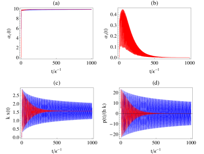
Figure 2: Cooling in standing wave cavity (blue) vs. ring cavity (red). Parameters $U_{0}=0.1\times\kappa$, $\Delta_{c}=-0.3\times\kappa$ and $\eta=10.3\times\kappa$. (a) Field amplitude of cosine mode compared to the standing-wave cavity mode. (b) Sine mode field amplitude. (c) particle localization (d) momentum of particle.

Notice that the standing wave cavity model ritsch97 can be reproduced by the above equations by setting $U_{cs}\left(x\right)=0$. This enables us to perform a comparison between the efficiency of the ring cavity cooling and that of a standing wave cavity with equal driving $\eta$. The numerical simulation results are presented in Fig.  2. The set of parameters that we consider $\kappa=1$ MHz, $k=2\pi\times 10^{6}$ m^-1, $m=77$ a.m.u, $U_{0}=0.1\times\kappa$, $\eta=10.3\times\kappa$ and initial momentum $5\hbar k$ is unrealistic in that a high value of $U_{0}$ around $100$ kHz is feasible with atoms but not with molecules. The purpose of the exaggeration in the choice of $U_{0}$ is to illustrate the advantage of ring-cavity cooling with large fields numerically since for smaller $U_{0}$ integration of Eqs. (4) is a computationally hard and long task. The situation presented in Fig. 2 is that of a particle trapped inside a single potential well and cooled on a timescale of order $500\times\kappa^{-1}$ (as seen in Fig.  2d) which is much faster than the corresponding standing-wave cavity cooling time. The detuning has been chosen at the value of $\Delta=-0.3\times\kappa$ which is close to the trapping frequency of the particle in the cosine mode, choice that will be elucidated in the next Section.

IV The strong confinement limit

We will focus now on the quantum dynamics of this system in steady state for strong pump and deep trapping. We drop the index of $\alpha_{c}$ and denote by $\alpha$ the steady state amplitude of the cosine mode, which we assume to be large and real (which can be guaranteed by the proper choice of phase of $\eta$). For small coupling $U_{0}\ll\kappa$ we approximate it by $\alpha=\left|\eta\right|/\sqrt{\kappa^{2}+\Delta^{2}}$. Note that as discussed in the following sections this only makes sense in the cooling regime, where we can expect a steady state state of the coupled system with a finite particle energy as well.

In the limit $\alpha\gg 1$, one can ignore the term $a^{\dagger}a\sin^{2}k\hat{x}$ in Eq. (2) as being small compared to the $\alpha^{2}\cos^{2}k\hat{x}$ term, so that the cosine mode creates a deep periodic trapping potential. Assuming good localization of the particle ($kx\ll 1$) at the field maxima, one can expand $\cos^{2}k\hat{x}\simeq 1-k^{2}\hat{x}^{2}$ and $\sin 2k\hat{x}\simeq 2k\hat{x}$. The Hamiltonian of Eq. (2) then becomes

$$H=\left[\frac{\hat{p}^{2}}{2m}+\frac{1}{2}m\omega_{m}^{2}\hat{x}^{2}\right]-\hbar\Delta a^{\dagger}a-\hbar U_{0}^{\prime}(a+a^{\dagger})\hat{x},$$ (5)

with effective harmonic trapping frequency $\omega_{m}^{2}=2\hbar U_{0}\left(k\alpha\right)^{2}/m$ and rescaled effective interaction strength $U_{0}^{\prime}=U_{0}k\alpha$. This interaction rescaling is similar to the case of optomechanical systems with mirrors or membranes in the limit of large photon numbers Wilson-Rae-theory-07 ; genes-ground-08 ; Marquardt-quantum-07 where a fundamentally small coupling is collectively enhanced with the square root of the photon number. Note that a similar collective effect could be in principle used also for single standing wave mode cooling. However, as the atoms then are confined close to a maximum of this mode, where its derivative is zero we only get a coupling being second order in $x$, which is intrinsically much smaller leading to a weaker cooling effect.

IV.1 Fourier space analysis

Reducing the operators to dimensionless quadratures, $\hat{Q}=\hat{x}/x_{zpm}$ and $\hat{P}=\hat{p}/p_{zpm}$ (where the ground state position uncertainty $x_{zpm}=\sqrt{\hbar/m\omega_{m}}$ and its corresponding momentum spread $p_{zpm}=\hbar/x_{zpm}$), one can write linearized Langevin equations in the form:

$$\frac{d}{dt}a(t) = (i\Delta-\kappa)a(t)+i\bar{U}_{0}Q+a_{in},$$ (6a)

$$\frac{d}{dt}a^{\dagger}(t) = (-i\Delta-\kappa)a^{\dagger}(t)-i\bar{U}_{0}Q+a_{in}^{\dagger}$$ (6b)

$$\frac{d}{dt}Q(t) = \omega_{m}P,$$ (6c)

$$\frac{d}{dt}P(t) = -\omega_{m}Q+\bar{U}_{0}a+\bar{U}_{0}a^{\dagger}.$$ (6d)

The new coupling strength is

$$\bar{U}_{0}=x_{zpm}U_{0}^{\prime}=\left(kx_{zpm}\right)\times\left(U_{0}\alpha\right).$$ (7)

Note that the implicit dependence of $\bar{U}_{0}$ on $\alpha$ through the Lamb-Dicke parameter $kx_{zpm}\sim\omega_{m}^{-1/2}\sim\alpha^{-1/2}$ reduces the collective enhancement scaling to $\bar{U}_{0}\sim\alpha^{1/2}$. The difference to the typical scaling with $\alpha$ as in optomechanical setups lies in the fact that the same field that mediates the interaction, namely the cosine mode, is also responsible with creating the optical trap.

One can proceed to solve Eqs. (6) as in Wilson-Rae-theory-07 by deriving an effective reduced master equation for the motional degree of freedom or as in genes-ground-08 by analytically deriving spectra of correlations of operators and integrating to find variances in steady state. For example, starting from Eqs. (6) one can derive the spectrum of the $Q$ variance as $\left\langle Q\left(\omega\right)Q\left(\omega^{\prime}\right)\right\rangle=S_{Q}\left(\omega\right)\delta\left(\omega+\omega^{\prime}\right)$ and integrate to find $\left(\Delta Q\right)^{2}\simeq n_{at}+1/2$. We state in the following results obtained via any of these methods in the perturbative limit where $\bar{U}_{0}\ll\kappa$. The physics of cooling in this regime is elucidated by considering the scattering rates into optical sidebands

$$A\left(\omega\right)=\frac{\kappa\bar{U}_{0}^{2}}{\kappa^{2}+\left(\omega-\Delta\right)^{2}}.$$

An effective cooling rate is obtained as a difference between Antistokes and Stokes rates

$$\Gamma=A\left(\omega_{m}\right)-A\left(-\omega_{m}\right)$$ (8)

and the final occupancy of

$$n_{at}=\frac{\kappa^{2}+\left(\omega_{m}+\Delta\right)^{2}}{-4\omega_{m}\Delta}$$ (9)

is optimized to $\left(\kappa/2\omega_{m}\right)^{2}$ under the condition of optimal cooling $\Delta=-\omega_{m}$.

The spectrum of the field fluctuations can be easily shown to be proportional to the spectrum of motion $n_{a}\left(\omega\right)=A\left(\omega\right)S_{Q}\left(\omega\right)$. Integration leads to a simple expression:

$$n_{a}=\frac{A\left(\omega_{m}\right)A\left(-\omega_{m}\right)}{4\kappa\Gamma}=\frac{U_{0}}{-8\Delta}.$$ (10)

The apparent divergence in the expressions of $n_{at}$ and $n_{a}$ is related to the fact that for very small detunings one leaves the cooling regime gangl-cold-00 and the particle spreads out over a spatial range beyond the validity of the linearization. This behavior shows up as well in the numerical simulations of the full model (see Sec. V) and is more thoroughly analyzed in Sec. IV.2, where we show that the validity of our linearized treatment imposes that $\left|\Delta\right|$ cannot be smaller than the recoil frequency $\omega_{rec}=\hbar k^{2}/2m$.

IV.2 Validity of tight confinement treatment

The validity of the linearized treatment requires localization of the particle within an optical wavelength which in a first approximation imposes that $kx_{zpm}\ll 1$. In other words this requires that the trap frequency $\omega_{m}$ be much larger than the recoil frequency $\omega_{rec}=\hbar k^{2}/2m$,

$$\omega_{rec}\ll\omega_{m}\text{.}$$

Moreover, localization of the particle in the final state described by the occupancy $n_{at}$ of Eq. (9) requires that the spread of the final state (a thermal state) is also smaller than a wavelength, i.e, $kx_{zpm}\sqrt{n_{at}}<1$. Assuming $\Delta$ small compared to $\omega_{m}$ and $\omega_{m}$ of the order of $\kappa$, this condition is equivalent to

$$\left|\Delta\right|>\omega_{rec}\text{.}$$

As discussed in a number of papers Wilson-Rae-theory-07 ; genes-ground-08 ; Marquardt-quantum-07 , sideband cooling works best when the Antistokes sideband is maximally enhanced, i.e. when $\Delta=-\omega_{m}$. This implicitly sets a value for $\omega_{m}$

$$\omega_{m}^{2}=\frac{1}{2}\kappa^{2}\left[\sqrt{1+\frac{16\omega_{rec}U_{0}\eta^{2}}{\kappa^{4}}}-1\right].$$

Moreover, to resolve the sidebands one has to also ask that $\omega_{m}>\kappa$ which is equivalent to

$$2\frac{\omega_{rec}U_{0}\eta^{2}}{\kappa^{4}}>1.$$

One can see that this requirement is not inconsistent with the assumption of our perturbative treatment, namely $\bar{U}_{0}\ll\kappa$, which, under the assumption that $\omega_{m}$ is of the order of $\kappa$ can be reexpressed as

$$2\frac{\omega_{rec}U_{0}\eta^{2}}{\kappa^{4}}\ll\frac{\kappa}{U_{0}}\text{,}$$

and which can be easily fulfilled for single molecules given the smallness of the coupling $U_{0}$.

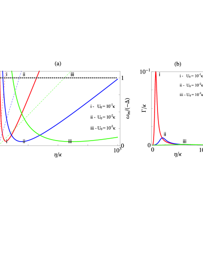
Figure 3: Atomic occupancy (a) and cooling rate (b) as a function of increasing $\eta$ for fixed $\Delta=-2\kappa$. The minima of the full lines (i, ii and iii) occur at the point where the 3 dashed lines (that show $-\omega_{m}/\Delta$) intersect the dashed black line of value 1, i.e. when the optimal sideband cooling condition is fulfilled. The cooling rates are also optimal, as expected, at values of $\eta$ which ensure $\omega_{m}=-\Delta$.

IV.3 Coupled equations for operator expectation values

Starting from Eq. (1) where the linear dynamics is given by the simplified Hamiltonian of Eq. (5) and following the ideas shown in gangl1999collective one can derive a closed set of linear differential equations containing expectation values of pairwise operator products only. These can be solved dynamically and also exact steady state values for

$(\langle{a^{\dagger}a}\rangle,\langle{Q^{2}}\rangle,\langle{P^{2}}\rangle)$ can be deduced:

$$\frac{d}{dt}\langle{a^{\dagger}a}\rangle = -2\kappa\langle{a^{\dagger}a}\rangle-i\bar{U}_{0}(\langle{aQ}\rangle-\langle{a^{\dagger}Q}\rangle),$$ (11a)

$$\frac{d}{dt}\langle{Q^{2}}\rangle = \omega_{m}\langle{\mathcal{A}}\rangle,$$ (11b)

$$\frac{d}{dt}\langle{\mathcal{A}}\rangle = 2\omega_{m}(\langle{P^{2}}\rangle-\langle{Q^{2}}\rangle)+$$ (11c)

$$2\bar{U_{0}}(\langle{aQ}\rangle+\langle{a^{\dagger}Q}\rangle),$$

$$\frac{d}{dt}\langle{P^{2}}\rangle = -\omega_{m}\langle{\mathcal{A}}\rangle+2\bar{U}_{0}(\langle{aP}\rangle+\langle{a^{\dagger}P}\rangle),$$ (11d)

$$\frac{d}{dt}\langle{aQ}\rangle = \omega_{m}\langle{aP}\rangle-(\kappa-i\Delta)\langle{aQ}\rangle+i\bar{U}_{0}\langle{Q^{2}}\rangle,$$ (11e)

$$\frac{d}{dt}\langle{aP}\rangle = (-\kappa+i\Delta)\langle{aP}\rangle-\omega_{m}\langle{aQ}\rangle+$$ (11f)

$$\bar{U}_{0}\left(\langle{a^{\dagger}a}\rangle+1/2+\langle{a^{2}}\rangle+\frac{i}{2}\langle{\mathcal{A}}\rangle\right),$$

$$\frac{d}{dt}\langle{a^{2}}\rangle = -2(\kappa-i\Delta)\langle{a^{2}}\rangle+2i\bar{U}_{0}\langle{aQ}\rangle,$$ (11g)

where $\langle{\mathcal{A}}\rangle=\langle{QP+PQ}\rangle$. One can therefore derive steady-state solutions from this set of coupled equations for the motional quadratures and intracavity photon number

$$\langle{a^{\dagger}a}\rangle=-\frac{\bar{U}_{0}^{2}(\Delta^{2}+\kappa^{2})}{4\omega_{m}\Delta(\kappa^{2}+\Delta^{2})+8\bar{U}_{0}^{2}\Delta^{2}},$$

$$\langle{Q^{2}}\rangle=-\frac{(\kappa^{2}+\omega_{m}^{2}+\Delta^{2})(\kappa^{2}+\Delta^{2})+2\bar{U}_{0}^{2}\omega_{m}\Delta}{4\omega_{m}\Delta(\kappa^{2}+\Delta^{2})+8\bar{U}_{0}^{2}\Delta^{2}}$$ (12)

$$\langle{P^{2}}\rangle=-\frac{(\kappa^{2}+\omega_{m}^{2}+\Delta^{2}+2\bar{U}_{0}^{2}\Delta/\omega_{m})(\kappa^{2}+\Delta^{2})+2\bar{U}_{0}^{2}\omega_{m}\Delta}{4\omega_{m}\Delta(\kappa^{2}+\Delta^{2})+8\bar{U}_{0}^{2}\Delta^{2}}$$ (13)

which in the limit where $\bar{U}_{0}\ll\kappa$ are approximated by the expressions listed in Sec. IV.1. The method is a little more laborious, but instructive since it provides one with results that hold for arbitrary coupling strength $U_{0}$ and with some insight into the physics of the cooling process as seen from the relation derived for the intracavity photon number

$$\langle{a^{\dagger}a}\rangle=-\frac{\omega_{m}}{2\Delta}(\langle{Q^{2}}\rangle-\langle{P^{2}}\rangle).$$

This shows that $n_{a}$ is directly proportional to the imbalance between the uncertainties $\langle{Q^{2}}\rangle$ and $\langle{P^{2}}\rangle$, thus giving a good measure of the ’squashing ’ of the uncertainty disk characteristic of a coherent state (or vacuum).

Moreover, the exact expressions of $\langle{Q^{2}}\rangle$ and $\langle{P^{2}}\rangle$ allow us to make a clear investigation of the feasibility of our molecule cooling scheme, i.e., into the cooling occupancy and rates with diminishing $\bar{U}_{0}$. As seen in Fig. 3, for a fixed $\Delta=-2\kappa$, one can increase the cavity input power to reach a point of optimal cooling where the occupancy is minimized as the cooling rate is maximized, and which is given by the condition $\omega_{m}=-\Delta$. This is valid for any arbitrarily small $U_{0}$. However, as $U_{0}$ is set to smaller values, the cooling rates are becoming unrealistically small. Setting the optimal cooling condition, $\omega_{m}=-\Delta$, the results of Fig.  4(a) are straightforward, showing that the occupancy asymptotically tends to 0 with increasing $\eta$. Investigating the analytical expression for $\Gamma$ as given in Eq.  (8), we see that in the unresolved sideband regime where $\omega_{m}\ll\kappa$, the scaling is with $\eta^{3}$ while deep in the resolved sideband regime where $\kappa\ll\omega_{m}$ the scaling drops to $\sqrt{\eta}$. This is clearly illustrated in Fig. 4(b) where the turning point occurs around an $\eta$ for which $\omega_{m}\approx\kappa$.

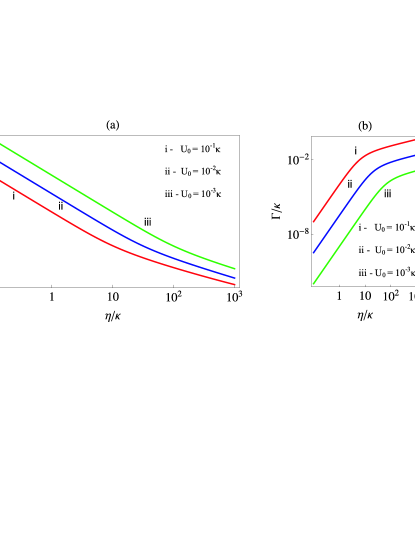
Figure 4: Log-log plots of atomic occupancy (a) and cooling rate (b) as a function of increasing $\eta$ for variable $\Delta$ that is dynamically changed to fulfill the optimal cooling condition $\omega_{m}=-\Delta$. The occupancy goes to 0 as expected for large $\eta$ as the system goes deep into the resolved sideband regime (as seen in (a)). The cooling rate increases at first with $\eta^{3}$ and after entering the resolved sideband regime, its scaling drops to $\sqrt{\eta}$. The illustrations are for 3 values of $U_{0}$ and clearly show that small final occupancies can still be obtained even with small $U_{0}$, however, at the expense of drastic increases in the cooling times.

V Numerical simulations

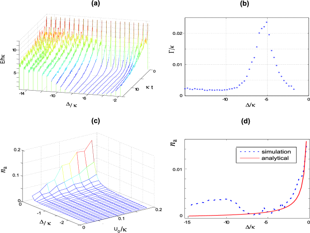
Figure 5: For a), b) and c), parameters are $U_{0}=0.01\times\kappa$ and $\omega_{m}=6\kappa$. a) Time dependence of average kinetic energy (mean over 100 trajectories) of the particle in units of $\hbar\kappa$ as a function of detuning. b) Cooling rate as a function of detuning. c) Simulated time averaged photon number in steady state as a function of detuning and coupling strength. d) Simulated and theoretical average sine mode photon number in steady state calculated in the linearized model as a function of detuning for $U_{0}=\kappa/20$.

After having demonstrated the key physical mechanisms present in the dynamics using different approximative analytical treatments, we will now check the range of validity of these results by a numerical solution of the full quantum model. The quantum dynamics can be efficiently approximated using time dependent Monte Carlo wavefunction simulations of the full coupled atom field system. Here we can conveniently make use of our established previously developed C++QED simulation package C++qed ; vukics2007c++ . Due to symmetry we can limit position space to one optical wavelength and truncate the photon numbers of the field modes sufficiently above the expected mean values, so that the overall size of the Hilbert space stays easily tractable. For very large pump photon numbers, the cosine mode dynamics can be approximated by a coherent field, so that only two quantum degrees of freedom have to be explicitly treated. This allows for even faster simulation and averaging over a large number of trajectories.

V.1 Cooling rates and steady state temperature

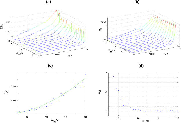
Figure 6: Fixed parameters are $U_{0}=\kappa/400$ and $\Delta=-\omega_{m}$. a) Averaged particle kinetic energy over 500 trajectories as a function of time for increasing trapping frequency starting with initial kinetic energy of $E_{k}\approx 25\hbar\kappa$. b)Average steady state photon number in sine-mode. We see the decrease associated with the better localization in a deeper trapping potential. c) Dots give the cooling rate $\gamma$ averaged over 500 trajectories. The solid line shows the expected power dependence derived from the linearized model above. d) Final steady state oscillator occupation number after a time $\kappa t=300$.

As a first step we confirm the efficiency of cooling as a function of cavity detuning by starting with a particle in a highly excited state and calculating its average energy loss as function of time for varying detuning between pump and cavity resonance. The kinetic energy as function of time is shown in Fig. 5(a). Close to optimal detuning $\Delta$ of we see a fast decay towards the ground state kinetic energy $\hbar\omega_{m}/4$ with an optimal value of the detuning near $\Delta=-\omega_{m}$. This value is different from the optimal value for $\Delta\approx-\kappa$ obtained for weak field cavity cooling and is characteristic for the optomechanical cooling limit where the mechanical oscillation frequency of the particle is bigger than the cavity linewidth $\kappa$. Less cooling or even heating occurs for small detunings in contrast with the optomechanical model predictions; the reason is the breakdown of the tight confinement model as explained in Sec.  IV.2. A central important quantity for the usefulness of this cooling method is the corresponding cooling rate, which we plot in Fig. 5(b). It also peaks near the sideband frequency $\omega_{m}$ and reaches almost the order of magnitude of $\kappa$ well above $U_{0}$, which gives a practically quite useful timescale.

Let us mention here that the simulations also give the steady state energy as a function of coupling strength $U_{0}$ and detuning. We find that for sufficiently large detuning we get ground state cooling also for very small coupling $U_{0}$. However, as expected for smaller $U_{0}$ the timescale to reach the ground state gets longer. This is different from a standard optomechanics setup, where the mirror is additionally coupled to a thermal reservoir and the cooling rate itself largely determines the final temperature. The corresponding simulation results are in good agreement with the analytic results obtained above.

Here we will show another aspect of this. As the cooling is connected to scattering of photons into the sine mode, its photon number $n_{a}$ directly provides information on the particle’s state and in particular on its temperature. The dependence of the sine-mode photon number $n_{a}$ on detuning and coupling strength is shown in Fig. 5(c). It shows the predicted divergence at low detunings and agrees fairly well with the theoretical prediction from the linearized model above (See Fig. 5(d)), as in steady state the particle is well localized and linearization is justified.

Let us note that that the sine-mode scattered photon number, i.e. $n_{a}$ is independent of mass, which is surprising according to a simple logic that a better localized particle would be expected to scatter less into the sine-mode, which is zero at its trapping point. We now add a direct comparison of the simulated and theoretically predicted average photon number in Fig. 5(d). While for smaller detunings the agreement is excellent, we see that at larger detunings the simulation predicts higher numbers. To a large extend this reflects the fact that even after a simulation time of $\omega_{rec}t=1000$ the system has not reached its steady state value.

As next important issue we confirm the possibility of fast cooling even for very small coupling. For this purpose we show how the initial kinetic energy of a particle decays for small effective coupling $U_{0}=\kappa/400$ with increasing pump power. A deeper potential leads to higher trapping frequencies, faster cooling and better final particle localization. This is visible in Fig. 6(a), where we plot the loss of kinetic energy of a trapped particle as an average over 500 trajectories. We see that for the same initial kinetic energy we get much faster relaxation with higher trapping frequency. This behavior gets even more obvious, if one looks at the average occupation number of the trapped particle as function of time. While the final kinetic energy first drops due to better cooling but then increases with higher $\omega_{m}$ due to the increasing zero point energy of the particle, the average particle vibrational excitation in the trap continuously drops and reaches almost zero for deep traps. Of course in practise, at some point one gets limited by the very small but yet nonzero spontaneous emission rate, which will induce heating and particle loss on a very long time scale.

The cooling can be directly and nondestructively monitored in the scattered photon number shown Fig. 6(b) which directly reflects better ground state cooling with increasing trap depth. The detailed correspondence of the two quantities as calculated in the analytical section can be even more clearly seen in individual trajectories as discussed in the next section.

One central question is the efficiency of the cooling for very far off resonance excitation, where the coupling of the particle to the field modes gets small. Here we can make use of very high pump mode photon numbers as in optomechanics. Extracting the corresponding decay rate from an exponential fit in Fig. 6(c) we see its nonlinear increase with $\omega_{m}$ in accordance with the expected behavior form the linearized model.

To show that this faster cooling does not enhance the diffusion significantly, we also plot the long time average of the oscillator excitation number in Fig. 6(d), which predicts ground state cooling at large $\omega_{m}$.

As a bottom line we clearly see that with sufficient power in the cosine mode to generate large mechanical trapping frequencies we can get fast molecular cooling despite very small coupling. As the induced photon number in the sine mode still stays small, we expect that this result holds even for more particles cooled simultaneously as long the photon number in the sine mode does not increase too much. We plan to study this scaling in more detail in the future.

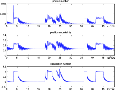
Figure 7: Single trajectory expectation values showing the particle occupation number, the photon number in the sine mode and the particles position uncertainty as a function of time for $\Delta=-2\kappa$ and other parameters as in Fig. 5.

V.2 Quantum Jumps

One very useful advantage of the Monte Carlo simulation approach is that besides averages and expectation values one can also look at individual trajectories, from which one can get interesting clues on the underlying dynamics and direct hints for the expected experimental data. In Fig. 7 we show a time window of the results of a typical trajectory as used above to find averages. In order to exhibit interesting dynamics we have chosen the case of a bit lower than optimum detuning $\Delta=-2\kappa<\omega_{m}$ still yielding a non-vanishing occupation of the first excited trap level. In the simulation we continuously monitor the photons leaving the sine-mode. As we always know the momentary atom-field wavefunction, we can easily show its correlation with any other system variable.

As expected we see a clear correspondence between the time evolution of the atomic position uncertainty and occupation number and the average photon number in the sine mode. Note that after reaching the ground state the system shows striking and clear quantum jumps between the lowest and first excited state. While it spends long periods in the ground state we see sporadic jumps to the first excited state where the particle remains for surprisingly long time until jumping back. This should be related with a symmetry change in the particle wave function during such a jump. While such jumps are forbidden in a standing wave cavity setup, they attain a finite probability in a ring cavity horak-dissipative-01 , where spontaneous shifts of the trap minimum allow to break the mirror symmetry of the trap. As these fluctuations are rather rare, the first excited state, once excited, is much more long lived than the second excited trap state, which possesses the same symmetry as the ground state. The observation of such quantum jumps thus would clearly reveal the quantum nature of the molecule’s center of mass dynamics.

VI Discussion

Lets now add some remarks on the effects of the spontaneous photon scattering rate $\gamma$. Naturally a molecule is not a simple two-level system. Nevertheless considering a single ground state and one manifold of excited states centered around $\omega_{a}$ with an energy spread bandwidth smaller than the laser detuning $\Delta_{a}\,$, can well describe the induced polarization dynamics. For weak saturation a two-level approach with an effective dipole matrix element is then sufficient. In the limit of $\Delta_{a}\gg\gamma$, the induced molecular polarization can be decomposed into real and imaginary parts describing dispersion (proportional to $U_{0}$) and absorption (proportional to $\gamma_{0}=\gamma g^{2}/\Delta_{a}^{2}$). To lowest order, $\gamma_{0}$ supplements the coupling strength $\bar{U}_{0}$ in Eqs. (6) with an imaginary part $i\bar{\gamma}_{0}=i\left(kx_{zpm}\right)\times\left(\gamma_{0}\alpha\right)$. Within our model, this implies a renormalizing of the coupling strength from $\bar{U}_{0}$ to $\sqrt{\bar{U}_{0}^{2}+\bar{\gamma}_{0}^{2}}$. In view of $\bar{\gamma}_{0}\ll\bar{U}_{0}$, the effect is negligible.

A second effect is the diffusion of the momentum triggered by the spontaneously emitted photons. A rate proportional to $\bar{\gamma}_{0}\alpha^{2}\left(kx_{zpm}\right)^{2}$ up to a geometrical factor is obtained that can again be neglected based on the smallness of $\bar{\gamma}_{0}$ and the inhibition with the square of the Lamb-Dicke parameter.

One can extend Eqs. (6) to also include quantum fluctuations of the cosine mode. The fluctuations of this mode are close to those of the vacuum state with extra terms coming from the scattering of the sine mode photons off the molecule. Qualitatively this leads to a fluctuating trapping frequency $\omega_{m}$ (that is proportional to $\alpha^{2}$) and a fluctuating coupling strength $\bar{U}_{0}$. For a quantitative analysis, one can notice that in the regime which is optimal for cooling where $\Delta=-\omega_{m}$, the sine mode population is always close to zero (as shown in Eq. (10)) and backscattering into the cosine mode can be neglected. When operating close to resonance, surely a large $U_{0}$ can lead to a considerable number of photons in the sine mode and the back action and potential shift effects listed above have to be taken into account, for example by following an approach similar to the one in rabl-phase-09 .

As first noticed in vitali-optomechanical-07 , the linear optomechanical interaction described by Eqs. (6) can lead to entanglement between the two degrees of freedom: vibration of molecule and quadratures of the sine mode, owing to quadrature-quadrature interaction. In terms of the logarithmic negativity, a maximum value of around $0.4$ around the optimal cooling regime can be obtained and can be even surpassed by a proper filtering of the cavity output field as suggested in genes-robust-08 . As an advantage over the mirror-field entanglement scheme which is strongly affected by the thermal bath, the molecule-field entanglement is effectively obtained under zero temperature conditions.

VII Conclusions

In conclusion we have shown that the ring cavity setup allows for strong coupling between a molecule’s motion and the sine mode via scattering of sideband photons from the cosine mode into the sine mode. The low single molecule field coupling is enhanced by the large photon number of the strongly driven cosine mode. In this regime the dynamics is similar to the one described in typical optomechanical systems with mirrors or membranes and we predict fast cooling rates. In contrast to superradiant cooling chan2003observation ; salzburger2009collective we do not need large molecular ensembles from start but rely on a single particle cooling mechanism. The central technical challenge here seems to generate high enough intensities in a ring cavity to assure trap frequencies larger than the cavity linewidth even at very large pump detunings from any optical resonance. Here mirrors with a finesse over $F=1000$ and supporting megawatt intracavity power are needed. From the molecular side one would like to have a high polarizability per mass with very low absorption at the chosen operating frequency. In this case even ground state cooling of any polarizable object seems feasible in a suitable ring cavity. As for atoms it could also be hoped that cooling properties get even more favorable in cavities invoking even more modes as in a confocal setup cavcoolrev .

Acknowledgements - We acknowledge support from the EC (FP6 Integrated Project QAP, and FET-Open project MINOS) and Euroquam Austrian Science Fund project I119 N16 CMMC.

References

- (1) B. L. Lev et al, Phys. Rev. A 77, 023402 (2008).
- (2) P. Domokos and H. Ritsch, J. Opt. Soc. Am. 20, 1098 (2003).
- (3) P. Horak et al., Phys. Rev. Lett. 79, 4974 (1997).
- (4) G. Morigi et al., Phys. Rev. Lett. 99, 073001 (2007).
- (5) S. Deachapunya et al., The European Phys. J. D 46, 307 (2007).
- (6) T. Salzburger and H. Ritsch, New J. Phys. 11, 055025 (2009).
- (7) K. Murret et al., Phys. Rev. A 73, 63415 (2006).
- (8) Y. Zhang et al., Frontiers Phys. China 4, 190 (2009).
- (9) D. R. Leibrandt et al., Phys. Rev. Lett. 103, 103001 (2009).
- (10) S. Slama et al., Phys. Rev. Lett. 98, 53603 (2007).
- (11) J. Klinner et al., Phys. Rev. Lett. 96, 023002 (2006).
- (12) F. Brennecke et al., Science 322, 235 (2008).
- (13) H. W. Chan, A. T. Black and V. Vuletić, Phys. Rev. Lett. 90, 63003 (2003).
- (14) S. Groeblacher et al., Nat. Phys. 5, 485 (2009).
- (15) A. Schliesser et al., Nat. Phys. 5, 509 (2009).
- (16) J. D. Thompson et al., Nature 452, 06715 (2008).
- (17) D. E. Chang et al., arXiv:0909.1548v2 (2009).
- (18) Oriol Romero-Isart et al., arXiv:0909.1469v2 (2009).
- (19) M. Gangl and H. Ritsch, Phys. Rev. A 61, 043405 (2000).
- (20) K. Murr, Phys. Rev. Lett. 96, 253001 (2006).
- (21) P. Domokos, P. Horak and H. Ritsch, J. Phys. B 34, 187 (2001).
- (22) I. Wilson-Rae et al., Phys. Rev. Lett. 99, 093901 (2007).
- (23) C. Genes et al., Phys. Rev. A 77, 033804 (2008).
- (24) F. Marquardt et al., Phys. Rev. Lett. 99, 093902 (2007).
- (25) M. Gangl and H. Ritsch, Phys. Rev. A 61, 011402 (1999).
- (26) This object oriented C++ package is freely available and documented at sourceforge.net.
- (27) A. Vukics and H. Ritsch, Euro. Phys. J. D, 44, 585 (2007).
- (28) P. Horak and H. Ritsch, Phys. Rev. A 63, 23603 (2001).
- (29) C. Genes, A. Mari, P. Tombesi, and D. Vitali, Phys. Rev. A 78, 032316 (2008).
- (30) P. Rabl et al., Phys. Rev. A 80, 063819 (2009).
- (31) D. Vitali et al., Phys. Rev. Lett. 98, 030405 (2007).