Intrinsic Spin and Orbital Hall Effects in Heavy Fermion Systems

Abstract

We study the intrinsic spin Hall effect (SHE) based on the orbitally degenerate periodic Anderson model, which is an effective model for heavy fermion systems. In the very low resistivity regime, the magnitude of the intrinsic spin Hall conductivity (SHC) is estimated as $2000\sim 3000\hbar{\rm e}^{-1}\Omega^{-1}{\rm cm}^{-1}$; It is about 10 times larger than that in Pt. Its sign is negative (positive) in Ce (Yb) compound systems with $f^{1}$ ($f^{13}$) configuration. Interestingly, the obtained expression for the SHC depends only on the density of conduction electrons, but is independent of the strength of the $c$-$f$ mixing potential and the mass-enhancement factor. The origin of the huge SHE is the spin-dependent Berry phase induced by the complex $f$-orbital wavefunction, which we call the “orbital Aharonov-Bohm effect”.

I Introduction

Spin Hall effect (SHE) is a phenomenon that an applied electric field induces a spin current in a transverse direction. It has been attracting a great deal of interest as a method for creating and detecting spin current. Recently, the SHE in metallic systems are intensively studied due to the interest for both the unsolved origin and the possibility of an application to spintronics device Murakami-SHE ; Sinova-SHE ; Inoue-SHE ; Rashba ; Raimondi ; Saitoh ; Valenzuela ; ZnSe ; Kimura

Recent intensive studies of the SHE in transition metals was initiated by the observation of the huge SHC in Pt Saitoh ; Kimura . To elucidate the origin of the huge SHE in transition metals, theoretical calculations of intrinsic SHE have been performed intensively Kontani-Ru ; Kontani-Pt ; Guo-Pt ; Tanaka-4d5d . The intrinsic SHE occurs in multiband metals with strong spin-orbit interaction (SOI) independently of impurities, which has a close relation to the intrinsic anomalous Hall effect (AHE) in ferromagnetic metals karplus . In ref. Tanaka-4d5d , the authors have revealed that huge SHEs are ubiquitous in multiorbital $d$-electron systems by calculating SHEs in various 4$d$ and 5$d$ transition metals. This study succeeds in explaining sophisticated and systematic experimental studies by Otani’s group Kimura . Therefore, it is strongly suggested that the intrinsic mechanism is dominant in transition metals.

The large SHE in transition metals is induced by the phase factor of the $d$-orbital wavefunction in the presence of the atomic SOI, which we call the “orbital Aharonov-Bohm (AB) effect” Kontani-OHE . The intrinsic SHC is predicted to be simply proportional to the spin-orbit polarization at the Fermi level $\langle{\bm{l}}\cdot{\bm{s}}\rangle_{\mu}$. According to the Hund’s rule, the SHC should be positive (negative) in transition metals with more (less) than half-filling. Moreover, occurrence of large orbital Hall effect (OHE), which is a phenomenon that large $d$-orbital Hall current is induced by the electric field, is also predicted theoretically in many transition metals Kontani-OHE . These fact suggests that a very large SHE and OHE may appear in $f$-electron systems compared to that in $d$-electron systems, since SHE and OHE are proportional to ${\langle{\bm{l}}\cdot{\bm{s}}\rangle_{\mu}}$ and $l$, respectively

In heavy fermion systems, very large AHE appears under the magnetic field Namiki ; Otop ; Sullow ; Hiraoka : In clean heavy fermion systems, anomalous Hall conductivity (AHC) $\sigma_{\rm SH}^{a}$ is independent of $\rho$ sufficiently below the coherent temperature $T_{0}$, whereas $\sigma_{\rm SH}^{a}\propto\rho^{-2}$ above $T_{0}$, which indicates that the intrinsic contribution is dominant in such clean samples. In ref. Kontani94 , they studied the AHE based on the orbitally degenerate periodic Anderson model (OD-PAM), which is an effective model for heavy fermion compounds. The obtained general expression has succeeded in explaining the huge AHC observed in heavy-fermion systems. Considering the close relationship between SHE and AHE, one might expect that huge SHE can be realized in heavy fermion systems.

In this paper, we study the intrinsic SHE based on the OD-PAM. It is found that the huge SHE in heavy fermion systems originates from the “orbital AB effect”, which is given by the spin-dependent Berry phase induced by the complex $f$-orbital wavefunction. In the low resistive regime, the SHCs in Ce- and Yb-compound systems are predicted to be about $2000\sim 3000\hbar e^{-1}\cdot\Omega^{-1}\text{cm}^{-1}$ in magnitude, which are one order larger than that the value observed in Pt. The sign of the SHC is negative (positive) in Ce (Yb) compound systems with $f^{1}$ ($f^{13}$) configuration, since the SHC is proportional to the spin-orbit polarization $\langle{\bm{l}}\cdot{\bm{s}}\rangle_{\mu}$ Kontani-OHE . The obtained expression for the SHC does not depend on the strength of the $c$-$f$ mixing potential nor the mass-enhancement factor. The SHC in $f$-electron systems will be measurable by using recently developed fabrication technique of high quality heavy fermion thin film Shishido .

Recently, present authors have studied the extrinsic SHE based on the orbitally degenerate single-impurity Anderson model (OD-SIAM) Tanaka-NJP . Using the Green functional method, we have derived both the skew scattering and side-jump terms analytically. It is found that the side-jump term derived in the OD-SIAM has a great similarity to the intrinsic term derived in the OD-PAM: The SHCs are simply proportional to ${\langle{\bm{l}}\cdot{\bm{s}}\rangle_{\mu}}$ and their magnitude are almost the same in both mechanisms. In section IV, we discuss the relationship between the intrinsic and the side-jump mechanisms.

II Model and Hamiltonian

In the present paper, we study the intrinsic SHE and OHE for both Ce- and Yb-compound heavy fermion systems based on the OD-PAM. In these systems, the number of $f$-electron or hole is unity, and the total angular momentum $J$ is $5/2$ or $7/2$. In the presence of the strong atomic SOI, the $J=7/2$ level is about 3000 K higher than the $J=5/2$ level. Therefore, we consider only $J=5/2$ ($J=7/2$) state in Ce³⁺ (Yb³⁺) ion with 4$f^{1}$ (4$f^{13}$) configuration. We note that $\bm{l}\cdot\bm{s}=\frac{1}{2}\left[J(J+1)-L(L+1)-S(S+1)\right]$ is given as follows:

$$\bm{l}\cdot\bm{s} = -2\ \ \text{for}\ \ J=5/2,{}$$

$$\bm{l}\cdot\bm{s} = \frac{3}{2}\ \ \text{for}\ \ J=7/2.$$ (1)

Here, we introduce the following OD-PAM Hamiltonian, which had been used to explain the large Van-Vleck magnetic susceptibility Kontani-VV and the small Kadowaki-Woods ratio Kontani-GKWR in heavy fermion systems with orbital degeneracy.

$$\hat{H} = \sum_{{\bm{k}}{\sigma}}{\varepsilon}_{{\bm{k}}}c^{\dagger}_{{\bm{k}}{\sigma}}c_{{\bm{k}}{\sigma}}+\sum_{{\bm{k}}M}E^{f}f^{\dagger}_{{\bm{k}}M}f_{{\bm{k}}M^{\prime}}{}$$ (2)

$$+\sum_{M{\bm{k}}{\sigma}}\left(V^{\ast}_{{\bm{k}}M{\sigma}}f^{\dagger}_{{\bm{k}}M}c_{{\bm{k}}{\sigma}}+V_{{\bm{k}}M{\sigma}}c^{\dagger}_{{\bm{k}}{\sigma}}f_{{\bm{k}}M}\right){}$$

$$+U\sum_{i,M\neq M^{\prime}}n^{f}_{iM}n^{f}_{iM^{\prime}},$$

where, $c^{\dagger}_{{\bm{k}}{\sigma}}$ is the creation operator of a conduction electron with spin ${\sigma}=\pm 1$. $f^{\dagger}_{{\bm{k}}M}$ is the operator of a $f$-electron with total angular momentum $J=5/2\ (7/2)$ and $z$-component $M\ (-J\leq M\leq J)$ for Ce³⁺ (Yb³⁺). ${\varepsilon}_{{\bm{k}}}$ is the energy for $c$-electrons, $E^{f}$ is the localized $f$-level energy, and $U$ is the Coulomb interaction for $f$-electrons. $V_{{\bm{k}}M{\sigma}}$ is the mixing potential between the $c$- and $f$-electrons, which is given by Kontani94

$$V_{{\bm{k}}M{\sigma}} = \sqrt{\frac{2}{2J+1}}\sqrt{4\pi}V_{f}\sum_{m}a^{M}_{m{\sigma}}Y^{m}_{l}({\theta}_{{\bm{k}}},\phi_{{\bm{k}}}),$$ (3)

where, $a^{M}_{m{\sigma}}$ is the Clebsh-Gordan (C-G) coefficient and $Y^{m}_{l}({\theta}_{{\bm{k}}},\phi_{{\bm{k}}})$ is the spherical harmonic function. Here, the C-G coefficient for $l=3$ is given by (for l=3)

$$a^{M}_{m{\sigma}} = -{\sigma}\left\{\left(7/2-M{\sigma}\right)/7\right\}^{1/2}\delta_{m,M-{\sigma}/2}\ \ \text{for}\ \ J=5/2,{}$$

$$a^{M}_{m{\sigma}} = \left\{\left(7/2+M{\sigma}\right)/7\right\}^{1/2}\delta_{m,M-{\sigma}/2}\ \qquad\text{for}\ \ J=7/2.{}$$

Here, the ${\bm{k}}$-dependence of $V_{f}$ is neglected due to the small radius of the $f$-orbital wave function. We also neglect the crystalline electric field splitting of $E^{f}$-level since its effect on the intrinsic Hall effect would not be essential AHE-CEF . Hereafter, we put $U=0$; the effect of Coulomb interaction on the SHC will be discussed in section IV.

From the expression of the C-G coefficient in eq. (II), we see that conduction electrons with $\uparrow$-spin mainly hybridize with $M=-5/2$ ($M=7/2$) for $J=5/2$($J=7/2$), which is consistent with the Hund’s rule: That is the spin and orbital angular momentum are parallel (antiparallel) for $J=5/2$ ($J=7/2$). We will show that the sign of the SHC is explained by the spin-orbit polarization Kontani-OHE . In the present study, we neglect the effect of crystalline electric field on $f$-orbitals, since it is small due to the small radius of the $f$-orbital wave function. Hereafter, we put $\hbar=1$.

In Fig. 1, we show the band structure of OD-PAM given in eq. (2). Here, $E^{\pm}_{{\bm{k}}}$ represents the hybridization bands given by $E^{\pm}_{{\bm{k}}}=\frac{1}{2}\left[({\varepsilon}_{{\bm{k}}}+E^{f})\pm\sqrt{({\varepsilon}_{{\bm{k}}}-E^{f})^{2}+4|V_{f}|^{2}}\right]$. In this study, we assume the metallic state, where the Fermi level $\mu$ lies in the $c$-$f$ hybridization band. In this figure, $k_{F}$ is the Fermi momentum and $\Delta\equiv E^{f}-\mu$.

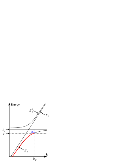
Figure 1: Band structure of the OD-PAM given in eq. (2). Here, $E^{\pm}_{{\bm{k}}}$ is the hybridization band.

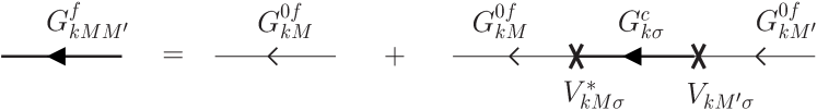
Figure 2: The diagrammatic expression for the Green function in eq. (LABEL:eq:Gf) Kontani94 .

Here, the conduction and $f$-electron Green functions for OD-PAM in the absence of the magnetic field are given by as follows Kontani94 :

$$G^{c}_{{\bm{k}}{\sigma}{\sigma}}({\omega}) = \left({\omega}+\mu-{\varepsilon}_{{\bm{k}}}-\sum_{M}\frac{{|V_{{\bm{k}}M{\sigma}}|^{2}}}{{\omega}+\mu-E^{f}_{M}}\right)^{-1},$$ (5)

$$G^{f}_{{\bm{k}}MM^{\prime}}({\omega}) = G^{0f}_{{\bm{k}}M}({\omega})\delta_{MM^{\prime}}{}$$

$$+ \sum_{{\sigma}}G^{0f}_{{\bm{k}}M}({\omega})V^{\ast}_{{\bm{k}}M{\sigma}}G^{c}_{{\bm{k}}{\sigma}}({\omega})V_{{\bm{k}}M^{\prime}{\sigma}}G^{0f}_{{\bm{k}}M^{\prime}}({\omega}).{}$$

We note that $G^{c}_{{\bm{k}}{\sigma}\bar{\sigma}}({\omega})=0$ Kontani94 . The diagrammatic expression for eq. (LABEL:eq:Gf) is given in Fig. 2. $G^{0f}$is the $f$-electron Green function without hybridization given as

$$G^{0f}_{{\bm{k}}M}({\omega}) = \frac{1}{{\omega}+\mu-E^{f}}.$$ (7)

Now, we consider the quasiparticle damping rate $\hat{\Gamma}({\omega})$, which is mainly given by the imaginary part of the $f$-electron self-energy, $\hat{\Sigma}_{{\bm{k}}}({\omega})$ in heavy fermion systems. In the dynamical mean-field approximation (DMFA), the self-energy is composed local $f$-Green function, $\frac{1}{N}\sum_{{\bm{k}}}G_{{\bm{k}}MM^{\prime}}({\omega})\equiv g({\omega})\delta_{MM^{\prime}}$, which is diagonal with respect to $M$ and is dependent of $M$ in the orbitally degenerate case Kontani-GKWR . Here, $N$ is the number of ${\bm{k}}$-points. Therefore, in the present study, we assume that $\hat{\Gamma}$ is diagonal with respect to $M$, and is independent of the momentum. Moreover, since $f$-electrons are degenerate in the present model, we assume that $\Gamma_{M}$ is approximately independent of $M$ and can be approximated as $\Gamma_{MM^{\prime}}=\gamma\delta_{MM^{\prime}}$, where ${\gamma}$ is a constant. In this study, we perform a calculation of the SHC using this constant ${\gamma}$ approximation. Then, the retarded (advanced) Green functions are given by

$$G^{c\rm{R(A)}}_{{\bm{k}}}({\omega}) = \left({\omega}+\mu-{\varepsilon}_{{\bm{k}}}-\frac{|V_{f}|^{2}}{{\omega}+\mu-E^{f}+(-)i{\gamma}}\right)^{-1},{}$$

$$G^{0f\rm{R(A)}}_{{\bm{k}}}({\omega}) = \left({\omega}+\mu-E^{f}+(-)i{\gamma}\right)^{-1}.$$ (8)

III Calculations of SHC and OHC

In this study, we calculate $\sigma_{\rm SH}$ based on linear response theory. According to Streda Streda , the SHC at $T=0$ in the absence of the current vertex correction (CVC) is given by $\sigma_{\rm SH}=\sigma_{\rm SH}^{I}+\sigma_{\rm SH}^{II}$, where

$$\sigma_{\rm SH}^{I} = \frac{1}{2\pi N}\sum_{{\bm{k}}}\text{Tr}\left[\hat{J}^{\rm{S}}_{x}\hat{G}^{\rm{R}}\hat{J}^{\rm{C}}_{y}\hat{G}^{\rm{A}}\right]_{{\omega}=0},$$ (9)

$$\sigma_{\rm SH}^{II} = \frac{-1}{4\pi N}\sum_{{\bm{k}}}\int_{-\infty}^{0}d{\omega}\text{Tr}\left[\hat{J}^{\rm{S}}_{x}\frac{{\partial}\hat{G}^{\rm{R}}}{{\partial}{\omega}}\hat{J}^{\rm{C}}_{y}\hat{G}^{\rm{R}}\right.{}$$ (10)

$$\qquad\left.-\hat{J}^{\rm{S}}_{x}\hat{G}^{\rm{R}}\hat{J}^{\rm{C}}_{y}\frac{{\partial}\hat{G}^{\rm{R}}}{{\partial}{\omega}}-\langle\rm{R}\leftrightarrow\rm{A}\rangle\right].$$

Here, $\sigma_{\rm SH}^{I}$ and $\sigma_{\rm SH}^{II}$ represents the Fermi surface term and the Fermi sea term, respectively.

In the present model, the charge current operator is given by $\hat{J}^{C}_{\mu}=-e\hat{v}_{{\bm{k}}\mu}$, where $-e\ (e>0)$ is the electron charge, and

$$\hat{v}_{{\bm{k}}\mu} = \sum_{{\sigma}}\frac{{\partial}}{{\partial}k_{\mu}}{\varepsilon}_{{\bm{k}}}c^{\dagger}_{{\bm{k}}{\sigma}}c_{{\bm{k}}{\sigma}}\sum_{{\sigma}M}\left\{\frac{{\partial}}{{\partial}k_{\mu}}V_{{\bm{k}}M{\sigma}}c^{\dagger}_{{\bm{k}}{\sigma}}f_{{\bm{k}}M}+{\rm h.c}\right\}.{}$$

Next, we explain the $s_{z}$-spin current operator $\hat{J}^{S}_{\mu}$. In the present model, $\hat{s}_{z}$ is given by

$$\hat{s}_{z} = \sum_{{\sigma}}\frac{{\sigma}}{2}c^{\dagger}_{{\bm{k}}{\sigma}}c_{{\bm{k}}{\sigma}}+\sum_{M}S_{M}f^{\dagger}_{M{\bm{k}}}f_{M{\bm{k}}},$$ (12)

where $S_{M}=\sum_{m{\sigma}}\frac{{\sigma}}{2}\left[a^{M}_{m{\sigma}}\right]^{2}$. It is straight forward to show that $S_{M}=-\frac{M}{7}$ ($\frac{M}{7}$) for $J=5/2$ $(J=7/2)$. Then, the spin current $\hat{J}^{S}_{\mu}\equiv\left\{\hat{v}^{c}_{{\bm{k}}\mu},\hat{s}_{z}\right\}/2$ is given by

$$\hat{J}^{S}_{\mu} = \sum_{{\sigma}}\frac{{\sigma}}{2}\frac{{\partial}{\varepsilon}_{{\bm{k}}}}{{\partial}k_{\mu}}c^{\dagger}_{{\bm{k}}{\sigma}}c_{{\bm{k}}{\sigma}}{}$$

$$+ \sum_{{\sigma}M}\left\{\frac{1}{2}\left(\frac{{\sigma}}{2}+S_{M}\right)\frac{{\partial}V_{{\bm{k}}M{\sigma}}}{{\partial}k_{\mu}}c^{\dagger}_{{\bm{k}}{\sigma}}f_{{\bm{k}}M}+\rm{h.c}\right\}.{}$$

In a similar way, the total angular momentum current operator, $\hat{J}^{J}_{\mu}\equiv\left\{\hat{v}^{c}_{{\bm{k}}\mu},\hat{J}_{z}\right\}/2$, is given by replacing $S_{M}$ in eq. (LABEL:eq:spin-current) with $M$. Then, the the orbital angular momentum current operator, $\hat{J}^{O}_{\mu}\equiv\hat{J}^{J}_{\mu}-\hat{J}^{S}_{\mu}$, is expressed as

$$\hat{J}_{\mu}^{O} = \left\{\hat{v}^{c}_{{\bm{k}}\mu},\hat{l}_{z}\right\}/2{}$$ (14)

$$= \sum_{{\sigma}M}\left\{\frac{1}{2}(M-S_{M})\frac{{\partial}V_{{\bm{k}}M{\sigma}}}{{\partial}k_{\mu}}c^{\dagger}_{{\bm{k}}{\sigma}}f_{{\bm{k}}M}+\rm{h.c}\right\}.$$

Then, the orbital Hall conductivity (OHC) $\sigma_{\rm OH}\equiv\langle J_{x}^{O}\rangle/E_{y}$ due to the OHE is given by $\sigma_{\rm OH}=\sigma_{\rm OH}^{I}+\sigma_{\rm OH}^{II}$, where $\sigma_{\rm OH}^{I}$ and $\sigma_{\rm OH}^{II}$ are respectively given by eqs. (9) and (10) by replacing $J^{S}_{x}$ with $J^{O}_{x}$.

Here, we study the velocity given by the $c$-$f$ mixing potential $V_{{\bm{k}}M{\sigma}}$ Kontani94 :

$$\frac{{\partial}V_{{\bm{k}}M{\sigma}}}{{\partial}k_{x}} = -i\left(M-\frac{{\sigma}}{2}\right)\frac{k_{y}}{k_{x}^{2}+k_{y}^{2}}V_{{\bm{k}}M{\sigma}}$$ (15)

$$+\frac{{\partial}}{{\partial}k_{x}}\left(V_{{\bm{k}}M{\sigma}}\alpha_{M,{\sigma}}^{*}\right)\alpha_{M,{\sigma}}$$

$$\equiv v_{x}^{a}+v_{x}^{b}.$$

Here, $v_{x}^{a}$ is the anomalous velocity given by ${\bm{k}}$-derivative of the phase factor $\alpha_{M,{\sigma}}=\rm{exp}\left\{i\left(M-\frac{{\sigma}}{2}\right)\phi_{k}\right\}$ in $V_{{\bm{k}}M{\sigma}}$. Figure 3 is a schematic view of the anomalous velocity $v^{a}\propto\nabla_{\bm{k}}\phi_{{\bm{k}}}$. Since $v^{a}_{x}\propto k_{y}$ and thus $\sum_{\bm{k}}v^{a}_{x}(\partial\epsilon_{\bm{k}}/\partial k_{y})\neq 0$, the anomalous velocity gives rise to the large SHE and AHE in heavy fermion systems. On the other hand, $v^{b}_{x}\propto k_{x}$ gives a normal velocity. In eqs. (9) or (10), the terms which contain single $v_{\mu}^{a}$ give rise to the SHC.

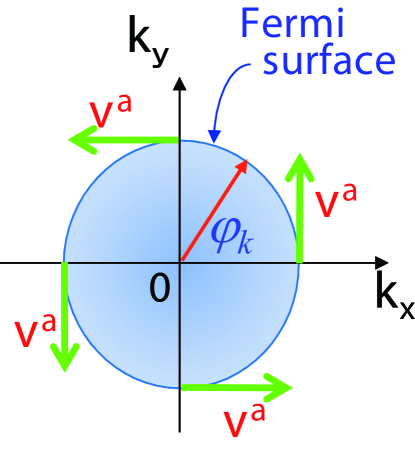
Figure 3: A schematic view of the anomalous velocity $v^{a}$.

III.1 Calculation of the Fermi surface term

Here, we calculate the SHC by neglecting CVC according to eqs. (9) and (10), using eqs. (III) and (III). $J^{C}_{\mu}$ and $J^{S}_{\nu}$ are composed of the conduction electron term ${\partial}{\varepsilon}_{{\bm{k}}}/{\partial}k_{\mu}\equiv{\partial}_{\mu}{\varepsilon}_{{\bm{k}}}$ and the hybridization term ${\partial}_{\mu}V_{{\bm{k}}}$. Fig. 4 shows the terms for $\sigma_{\rm SH}$ in which $\hat{J}^{S}_{x},\hat{J}^{C}_{y}$ is composed of zero or one ${\partial}_{mu}V_{{\bm{k}}}$. Fig. 4 (a) gives large SHC since ${\partial}_{\mu}V_{{\bm{k}}}$ includes the anomalous velocity in eq. (15). We note that the terms in 4 (b) that are composed only of ${\partial}_{x}{\varepsilon}_{{\bm{k}}}\cdot{\partial}_{y}{\varepsilon}_{{\bm{k}}}$ vanishes identically. Moreover, there exists the terms that are proportional to ${\partial}_{\mu}V_{{\bm{k}}}{\partial}_{\nu}V_{{\bm{k}}}$, as shown in Fig6. In Appendix B, we will show that these terms are much smaller than the contribution by Fig. 4 (a). Therefore, we here focus on the terms in Fig. 4 (a).

In this subsection, we derive the analytical expression for the Fermi surface term, since the Fermi surface term dominates over the Fermi sea term, as discussed in previous studies Kontani06 ; Kontani-Ru ; Kontani-Pt ; Tanaka-4d5d . The Fermi sea term will be derived in section III.2.

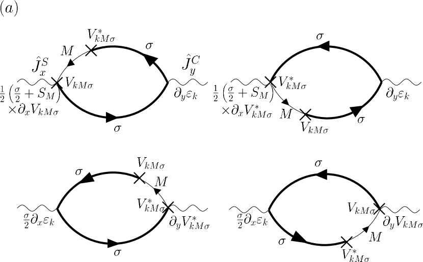
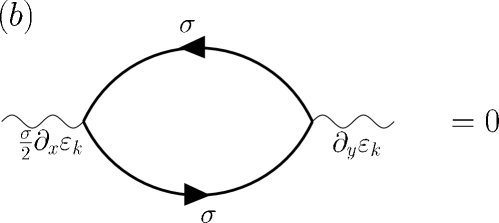
Figure 4: The diagrammatic expressions for $\sigma_{\rm SH}$. (a) The diagrammatic expressions for the dominant terms. (b) The diagrammatic expressions of the terms composed only of ${\partial}_{\mu}{\varepsilon}_{{\bm{k}}}$, which vanishes identically.

According to eqs. (9), (III) and (III), the Fermi surface term $\sigma_{\rm SH}^{I}$ for Fig. 4 (a) is given by

$$\sigma_{\rm SH}^{I} = \frac{-e}{2\pi N}\sum_{{\bm{k}}M{\sigma}}\frac{1}{2}\left(\frac{3{\sigma}}{2}+S_{M}\right){}$$

$$\times \left[\frac{{\partial}V_{{\bm{k}}M{\sigma}}}{{\partial}k_{x}}\frac{{\partial}{\varepsilon}_{{\bm{k}}}}{{\partial}k_{y}}V^{\ast}_{{\bm{k}}M{\sigma}}|G^{cR}_{{\bm{k}}}(0)|^{2}G^{0fR}_{{\bm{k}}}(0)+{\rm c.c.}\right].{}$$

Here, we confine ourselves to the case $J=5/2$ state corresponding to Ce ³⁺-ion. In section IV.1, we will discuss the case for $J=7/2$ state. Then, by using the following relationships

$$\sum_{M{\sigma}}M^{2}{|V_{{\bm{k}}M{\sigma}}|^{2}}=\frac{|V_{f}|^{2}}{2}\left(1+16\sin^{2}{\theta}\right),$$ (17)

$$\sum_{M{\sigma}}{\sigma}^{2}{|V_{{\bm{k}}M{\sigma}}|^{2}}=2|V_{f}|^{2},$$ (18)

$$\sum_{M{\sigma}}M{\sigma}{|V_{{\bm{k}}M{\sigma}}|^{2}}=|V_{f}|^{2}\left(1-4\sin^{2}{\theta}\right),$$ (19)

$$\frac{k_{y}}{k_{x}^{2}+k_{y}^{2}}=\frac{1}{k}\frac{\sin{\theta}\sin\phi}{\sin^{2}{\theta}},\ \frac{{\partial}{\varepsilon}_{{\bm{k}}}}{{\partial}k_{y}}=\frac{{\partial}{\varepsilon}_{{\bm{k}}}}{{\partial}k}\sin{\theta}\sin\phi,$$ (20)

eq. (III.1) is transformed as follows:

$$\sigma_{\rm SH}=\frac{-e}{2\pi N}\frac{52}{7}|V_{f}|^{2}\sum_{k}\frac{1}{k}\frac{{\partial}{\varepsilon}_{{\bm{k}}}}{{\partial}k}\frac{{\gamma}}{(\mu-E_{{\bm{k}}})^{2}+{\gamma}^{2}}|G^{c}_{{\bm{k}}}(0)|^{2},{}$$

where $k\equiv|{\bm{k}}|$.

Here, we analyze eq. (III.1) when ${\gamma}$ is small enough: In this case,

$$G^{cR}_{{\bm{k}}}(0) = \left(\mu-{\varepsilon}_{{\bm{k}}}-\frac{|V_{f}|^{2}}{\mu-E^{f}+i{\gamma}}\right)^{-1}{}$$ (22)

$$\simeq \left(\mu-\tilde{\varepsilon}_{{\bm{k}}}+i{\Gamma}_{c}\right)^{-1},$$

where $\displaystyle\tilde{\varepsilon}_{{\bm{k}}}={\varepsilon}_{{\bm{k}}}+\frac{|V_{f}|^{2}}{\mu-E^{f}}$, and $\displaystyle{\Gamma}_{c}=\frac{|V_{f}|^{2}}{(\mu-E^{f})^{2}}{\gamma}$. Since $\gamma/(x^{2}+\gamma^{2})=\pi\delta(x)$ for small $\gamma$, we obtain the following relationship:

$$|G^{cR}_{{\bm{k}}}(0)|^{2} = \frac{1}{(\mu-E_{{\bm{k}}})^{2}+{\Gamma}_{c}^{2}}{}$$ (23)

$$\simeq \frac{\pi}{{\Gamma}_{c}}\delta(\mu-E_{{\bm{k}}}).$$

Substituting above equation into eq. (III.1), we obtain the following relationship for small ${\gamma}$:

$$\sigma_{\rm SH} = \frac{-e}{2\pi N}\frac{52}{21}\sum_{k}\frac{1}{k}\frac{{\partial}{\varepsilon}_{{\bm{k}}}}{{\partial}k}\delta(\mu-E_{{\bm{k}}}).$$ (24)

Now, we approximate the conduction electron as free electron. Then, $\sigma_{\rm SH}^{I}$ for $J=5/2$ is given by

$$\sigma_{\rm SH}^{I} = -e\frac{26}{21}\frac{k_{F}}{2\pi^{2}}N_{FS}$$ (25)

$$= -\frac{e}{2\pi a}\frac{26}{21}N_{FS},$$

where $a$ is the lattice spacing and $N_{FS}$ represents the number of large Fermi surface. The first line in eq. (25) means that the SHC depends only on the density of conduction electron $n_{\rm c}=k_{\rm F}^{3}/3\pi^{2}$, except for $N_{FS}$. This result suggests that SHCs in $Ce$-compound heavy fermion systems take similar large negative values. The second line in eq. (25) is obtained by putting $k_{\rm F}=\pi/a$. When $a=4$Å, then $e/2\pi a\approx 1000\hbar e^{-1}\Omega^{-1}\rm{cm}$. If we assume that $N_{FS}=2\sim 3$, we obtain $\sigma_{\rm SH}=2000\sim 3000\hbar e^{-1}\Omega^{-1}$cm^-1 for Ce-compound system. Interestingly, the expression obtained above is independent of the strength of the $c$-$f$ mixing potential.

Next, we discuss the Fermi surface term for the OHC. By replacing $\hat{J}^{S}_{x}$ with $\hat{J}^{O}_{x}$ in eq. (9), $\sigma^{I}_{\rm OH}$ can be calculated in the same way as SHC. The obtained result is

$$\sigma^{I}_{\rm OH}=-\frac{7}{13}\sigma_{\rm SH}^{I}.$$ (26)

Thus, $\sigma^{I}_{\rm OH}$ shows a large positive value in Ce-compounds. In contrast, the relation $\sigma^{I}_{\rm OH}\gg|\sigma_{\rm SH}^{I}|$ is satisfied in transition metals since the SOI is weak and ${\langle{\bm{l}}\cdot{\bm{s}}\rangle_{\mu}}\ll 1$ Tanaka-4d5d .

III.2 Calculation of the Fermi sea terms

In this section, we derive the analytical expression for the Fermi sea term $\sigma_{\rm SH}^{II}$, and show that the Fermi surface term ($I$) dominates the Fermi sea term ($II$).

According to eqs. 10, III, and III, the Fermi surface term $\sigma_{\rm SH}^{II}$ for Fig. 4 (a) is given by

$$\sigma_{\rm SH}^{II} = \frac{e}{4\pi N}\sum_{{\bm{k}}M{\sigma}}\int^{0}_{-\infty}d{\omega}\ \frac{1}{2}\left(\frac{3{\sigma}}{2}+S_{M}\right){}$$ (27)

$$\times \left[\frac{{\partial}V_{{\bm{k}}M{\sigma}}}{{\partial}k_{x}}\frac{{\partial}{\varepsilon}_{{\bm{k}}}}{{\partial}k_{y}}\left\{\frac{{\partial}G^{fR}_{{\bm{k}}}({\omega})}{{\partial}{\omega}}G^{cR}_{{\bm{k}}}({\omega})-G^{fR}_{{\bm{k}}}({\omega})\frac{{\partial}G^{cR}_{{\bm{k}}}({\omega})}{{\partial}{\omega}}-\langle R\leftrightarrow A\rangle\right\}\right.{}$$

$$+\left.\frac{{\partial}V^{\ast}_{{\bm{k}}M{\sigma}}}{{\partial}k_{x}}\frac{{\partial}{\varepsilon}_{{\bm{k}}}}{{\partial}k_{y}}\left\{\frac{{\partial}G^{cR}_{{\bm{k}}}({\omega})}{{\partial}{\omega}}G^{fR}_{{\bm{k}}}({\omega})-G^{cR}_{{\bm{k}}}({\omega})\frac{{\partial}G^{fR}_{{\bm{k}}}({\omega})}{{\partial}{\omega}}-\langle R\leftrightarrow A\rangle\right\}\right].$$

Using the relations in eqs. (17) - (19), and performing the $M,\sigma$-summations in eq. (27), it is transformed as

$$\sigma_{\rm SH}^{II} = \frac{-e}{4\pi N}\sum_{{\bm{k}}}\left(-\frac{52}{7}\right)|V_{f}|^{2}\frac{1}{k}\frac{{\partial}{\varepsilon}_{{\bm{k}}}}{{\partial}k}{}$$

$$\text{Im}\left\{\int_{-\infty}^{0}\frac{d{\omega}}{\left[({\omega}-{\varepsilon}_{{\bm{k}}})({\omega}-E^{f}+i{\gamma})-|V_{f}|^{2}\right]^{2}}\right\}.{}$$

To perform the ${\omega}$-integration in eq. (III.2), we rewrite the integrand in eq. (III.2) as follows:

$$\left({\omega}+\mu-{\varepsilon}_{{\bm{k}}}\right)\left({\omega}+\mu-E^{f}+i{\gamma}\right)-|V_{f}|^{2}{}$$ (29)

$$= \left({\omega}+\mu-E^{+}_{{\bm{k}}}+i{\gamma}^{+}\right)\left({\omega}+\mu-E^{-}_{{\bm{k}}}+i{\gamma}^{-}\right),$$

where

$${\gamma}^{\pm}=\frac{{\gamma}}{2}\left(1\mp\frac{{\varepsilon}_{{\bm{k}}}-E^{f}}{E^{+}_{{\bm{k}}}-E^{-}_{{\bm{k}}}}\right).$$ (30)

Then, the ${\omega}$-integration in eq. (III.2) can be performed analytically as follows:

$$\int_{-\infty}^{0}\frac{d{\omega}}{\left({\omega}+\mu-E^{+}_{{\bm{k}}}+i{\gamma}^{+}\right)^{2}\left({\omega}+\mu-E^{-}_{{\bm{k}}}+i{\gamma}^{-}\right)^{2}}{}$$ (31)

$$= \frac{1}{\left[E^{+}_{{\bm{k}}}-E^{-}_{{\bm{k}}}-i\left({\gamma}^{+}-{\gamma}^{-}\right)\right]^{2}}\frac{E^{+}_{{\bm{k}}}+E^{-}_{{\bm{k}}}-2\mu-i\left({\gamma}^{+}+{\gamma}^{-}\right)}{\left(E^{+}_{{\bm{k}}}-\mu-i{\gamma}^{+}\right)\left(E^{-}_{{\bm{k}}}-\mu-i{\gamma}^{-}\right)}$$

$$+ \frac{2}{\left[E^{+}_{{\bm{k}}}-E^{-}_{{\bm{k}}}-i\left({\gamma}^{+}-{\gamma}^{-}\right)\right]^{3}}\ln\frac{E^{+}_{{\bm{k}}}-\mu-i{\gamma}^{+}}{E^{-}_{{\bm{k}}}-\mu-i{\gamma}^{-}}.$$ (32)

We analyze eqs. (31) and (32) when ${\gamma}$ is small: Since ${\rm Im}[\ln(x\pm i\gamma)]=\mp\pi\theta(x)$, the imaginary part of eqs. (31) and (32) is approximated as

$$\text{Im}\left\{\text{eq.}(\ref{eq:IIa-1})\right\} \approx \frac{\pi\delta\left(\mu-E^{-}_{{\bm{k}}}\right)}{\left(E^{+}_{{\bm{k}}}-E^{-}_{{\bm{k}}}\right)^{2}},$$ (33)

$$\text{Im}\left\{\text{eq.}(\ref{eq:IIb-1})\right\} \approx \frac{2\pi\theta\left(\mu-E^{-}_{{\bm{k}}}\right)}{\left(E^{+}_{{\bm{k}}}-E^{-}_{{\bm{k}}}\right)^{3}},$$ (34)

for Ce-compounds, where the Fermi level lies under $E^{f}$, as shown in Fig. 1. Substituting above equations into eq. (III.2), $\sigma_{\rm SH}^{IIa}$ and $\sigma_{\rm SH}^{IIb}$ is given by

$$\sigma_{\rm SH}^{IIa} = \frac{e}{2\pi N}\sum_{{\bm{k}}}\frac{52}{7}|V_{f}|^{2}\frac{1}{k}\frac{{\partial}{\varepsilon}_{{\bm{k}}}}{{\partial}k}\frac{\pi\delta\left(\mu-E^{-}_{{\bm{k}}}\right)}{\left(E^{+}_{{\bm{k}}}-E^{-}_{{\bm{k}}}\right)^{2}},$$ (35)

$$\sigma_{\rm SH}^{IIb} = \frac{-e}{2\pi N}\sum_{{\bm{k}}}\frac{52}{7}|V_{f}|^{2}\frac{1}{k}\frac{{\partial}{\varepsilon}_{{\bm{k}}}}{{\partial}k}\frac{2\pi\theta\left(\mu-E^{-}_{{\bm{k}}}\right)}{\left(E^{+}_{{\bm{k}}}-E^{-}_{{\bm{k}}}\right)^{3}}.$$ (36)

We will explain in Appendix A how to perform the ${\bm{k}}$-summations in eq. (36). In case of $|V_{f}|^{2}/(E^{f}-\mu)\gg 1$, final expressions for $\sigma_{\rm SH}^{IIa}$ and $\sigma_{\rm SH}^{IIb}$ are obtained as

$$\sigma_{\rm SH}^{IIa} = -\Lambda_{k_{F}}\sigma_{\rm SH}^{I},$$ (37)

$$\sigma_{\rm SH}^{IIb} = \sigma_{\rm SH}^{I}.$$ (38)

Here $\Lambda_{k_{F}}\equiv\frac{|V_{f}|^{2}}{(E^{+}_{k_{F}}-\mu)^{2}}a_{c}^{-1}$, and $\displaystyle a_{c}^{-1}\equiv\left.\frac{d{\varepsilon}_{{\bm{k}}}}{dE^{-}_{{\bm{k}}}}\right|_{E^{-}_{{\bm{k}}}=\mu}=1+\frac{|V_{f}|^{2}}{(\mu-E^{f})^{2}}$. Considering the relation $E^{+}_{k_{F}}\approx{\varepsilon}_{k_{F}}$ in Fig. 1, it is straight forward to show that $\Lambda_{k_{F}}\sim 1$ up to $O((\Delta^{2}/|V_{f}|)^{2})$. In this case, we obtain the following relationships for small ${\gamma}$:

$$\sigma_{\rm SH}^{I} \sim \sigma_{\rm SH}^{IIb}\sim-\sigma_{\rm SH}^{IIa},$$ (39)

$$\sigma_{\rm SH}^{I} \gg \sigma_{\rm SH}^{II}.$$ (40)

Therefore, two Fermi sea terms $\sigma_{\rm SH}^{IIa}$ and $\sigma_{\rm SH}^{IIb}$ almost cancel, and as a result, the Fermi surface term $\sigma_{\rm SH}^{I}$ gives a dominant contribution to the SHC Kontani06 ; Kontani-Ru ; Kontani-Pt ; Tanaka-4d5d . Note that the same relations also hold for the OHC, and the total OHC is mainly given by the Fermi surface term.

IV Discussions

IV.1 SHC and OHC in Yb-compound system

Now, we discuss the SHC for $J=7/2$, which corresponds to the case in Yb-compound systems.

To perform $M,{\sigma}$-summations, we use the following relations for $J=7/2$:

$$\sum_{M{\sigma}}M^{2}{|V_{{\bm{k}}M{\sigma}}|^{2}}=\frac{V_{f}}{2}\left(1+30\sin^{2}{\theta}\right),$$ (41)

$$\sum_{M{\sigma}}{\sigma}^{2}{|V_{{\bm{k}}M{\sigma}}|^{2}}=2V_{f},$$ (42)

$$\sum_{M{\sigma}}M{\sigma}{|V_{{\bm{k}}M{\sigma}}|^{2}}=V_{f}\left(1+3\sin^{2}{\theta}\right).$$ (43)

By using the above relationships, we can perform the calculation of $\sigma_{\rm SH}^{I}$ by following section III.1. As a result, $\sigma_{\rm SH}^{I}$ for $J=7/2$ takes a large positive value as

$$\sigma_{\rm SH}^{I} = e\frac{15}{14}\frac{k_{\rm F}}{2\pi^{2}}N_{FS}$$ (44)

$$= \frac{e}{2\pi a}\frac{15}{14}N_{FS}.$$

The second line in eq. (44) is obtained by putting $k_{\rm F}=\pi/a$. This result suggests that SHCs in Yb-compound heavy fermion systems take similar large positive values. We can also calculate the Fermi sea for $J=7/2$ by following section III.2. Then, we recognize the relationship in eqs. (39) and (40) for $J=7/2$.

In the same way, the OHC for $J=7/2$ state is given by

$$\sigma^{I}_{\rm OH}=\frac{14}{5}\sigma_{\rm SH}^{I}.$$ (45)

Therefore, we note that the sign of SHC is negative for $J=5/2$, it is positive for $J=7/2$, whereas the OHC is positive for both cases. These facts are consistent with the results obtained in 4$d$- and 5$d$ transition metals Tanaka-4d5d ; Kontani-OHE . In section IV.2, we will show that the sign of SHC is equal to the sign of the spin-orbit polarization $\langle{\bm{l}}\cdot{\bm{s}}\rangle_{\mu}$Kontani-OHE .

IV.2 Orbital Aharonov-Bohm Phase Factor

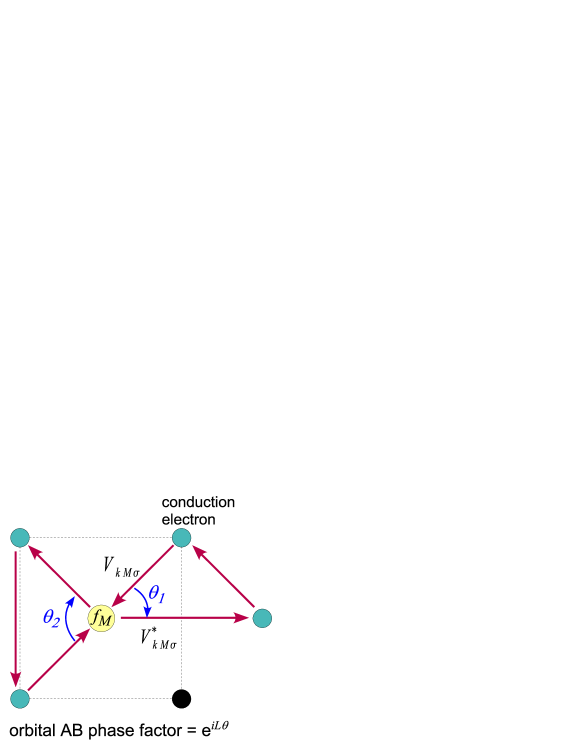
Figure 5: Effective Aharonov-Bohm phase in two-dimensional OD-PAM.

In previous sections, we have discussed the SHE based on the OD-PAM using the Green function method. In this section, we give an intuitive explanation for the origin of the huge SHE in heavy fermion systems. For this purpose, we consider the two orbital model with $M=\pm 5/2$, assuming the strong crystalline field. In the case of $J=5/2$, the $c$-$f$ mixing potential is given by $V_{M{\sigma}}(\hat{\bm{r}})\propto\left\{\sqrt{6}Y^{-3{\sigma}}_{3}(\hat{\bm{r}})\delta_{M,-5/2{\sigma}}+Y^{2{\sigma}}_{3}(\hat{\bm{r}})\delta_{M,5/2{\sigma}}\right\}$ in the real space representation: If we drop the second term, it can be approximated as $V_{M\sigma}({\bm{r}})\propto Y_{3}^{-3\sigma}(\hat{\bm{r}})\propto{\rm e}^{-3i\sigma\phi_{r}}$, where $\phi_{r}=\tan^{-1}(y/x)$.

In Fig. 5, two examples of the clockwise motion of the conduction electron along the nearest three sites [$f_{M}\rightarrow c\rightarrow c\rightarrow f_{M}$] are shown. Here, $\theta_{i}$ represents the angle between the incoming and outgoing electron. Therein, the electron acquires the phase factor ${\rm e}^{-3{\sigma}\theta}$ due to the angular dependence of the $c$-$f$ mixing potential in real space, $V_{M\sigma}(\hat{\bm{r}})$. This phase factor can be interpreted as the “orbital AB phase factor” at the $f$-site, which works as the effective magnetic flux $(-3{\sigma}\theta/2\pi)\phi_{0}$ through the area of the triangle. Here, $\phi_{0}=2\pi\hbar/e$ is the flux quantum. On the other hand, $V_{M{\sigma}}$ is approximately given by $V_{M{\sigma}}(\hat{\bm{r}})\propto{\rm e}^{3i{\sigma}\phi_{r}}$ for $J=7/2$. In this case, the effective magnetic flux per triangle is $(3{\sigma}\theta/2\pi)\phi_{0}$, which is opposite to that for $J=5/2$.

In summary, a conduction electron acquires the spin-dependent “orbital AB phase factor”, which originates from the spin-dependent $c$-$f$ hybridization in the presence of strong SOI. This is the origin of the huge SHE in heavy fermion systems. This consideration also explains the sign difference of the SHC between Ce- and Yb-compounds. Thus, the origin of the SHE in heavy fermion systems is well understood based on the simplified two-orbital model.

IV.3 The relationship between the intrinsic and side-jump terms

So far, we have studied the OD-PAM with translational invariance, and found that huge intrinsic SHC emerges. Here, we consider the depletion of $f$-electron. The quasiparticle damping rate $\gamma$ increases in proportion to the depletion ratio $x$. In the case of $x\ll 1$, the intrinsic SHC is independent of $x$ if $\gamma$ is smaller than the band splitting Kontani-Pt ; Tanaka-4d5d . In addition to the intrinsic term, the depletion may induce the extrinsic terms, that is, skew scattering term $\sigma_{\rm SH}^{\rm skew}$ and side-jump term $\sigma_{\rm SH}^{\rm sj}$.

In the dilute limit where $1-x\ll 1$, intrinsic term does not exist. In this case, present authors had studied the extrinsic SHE based on the orbitally degenerate single-impurity Anderson model Tanaka-NJP . For $k_{F}=\pi/a$ ($a$ is a lattice spacing), the expressions for skew scattering and side-jump terms are obtained as

$$\sigma_{\rm SH}^{\rm sj}=\frac{e}{2\pi a}\frac{2}{3}{\langle{\bm{l}}\cdot{\bm{s}}\rangle_{\mu}},$$ (46)

$$\sigma_{\rm SH}^{\rm skew}=\frac{e}{2\pi a}\delta_{2}\frac{1}{\gamma}{\langle{\bm{l}}\cdot{\bm{s}}\rangle_{\mu}},$$ (47)

for both $J=5/2$ (${\langle{\bm{l}}\cdot{\bm{s}}\rangle_{\mu}}=-2$) and $J=7/2$ (${\langle{\bm{l}}\cdot{\bm{s}}\rangle_{\mu}}=3/2$). Here, $\delta_{2}$ is a phase shift for $d$ partial wave. From the above equation, we find that the extrinsic term is proportional to the spin-orbit polarization ${\langle{\bm{l}}\cdot{\bm{s}}\rangle_{\mu}}$. In these two Anderson models, both intrinsic term $\sigma_{\rm SH}^{\rm int}$ and side-jump term $\sigma_{\rm SH}^{\rm sj}$ originate from the anomalous velocity that arises from the ${\bm{k}}$-derivative of the phase factor in the mixing potential. Here, we compare eqs. (25), (44), and (46). Very interestingly, the following relationship holds in a accuracy of $\pm 7.2$%:

$$\sigma_{\rm SH}^{\rm int}\approx\sigma_{\rm SH}^{\rm sj}$$ (48)

This fact indicates unexpected close relationship between the intrinsic term and the extrinsic side-jump term, and therefore it would be very difficult to distinguish these two mechanisms experimentally. This fact would be the reason why intrinsic (or side-jump) term are widely observed from single crystals to polycrystal or amorphous compounds.

V Summary

In this paper, we studied the intrinsic SHE and OHE based on the OD-PAM. We derived the analytical expression for the intrinsic SHC and OHC based on the linear response theory. Both SHC and OHC are mainly given by the Fermi surface term ($I$). The obtained results for Ce-compounds ($J=5/2$) are given by eqs. (25) and (26), and those for Yb-compounds ($J=7/2$) are given by eqs. (44) and (45). The SHCs for both compounds are approximately expressed by eq. (46). These results suggests that SHCs in $Ce$- ($Yb$-) compound heavy fermion systems take similar large negative (positive) values; $2000\sim 3000\hbar e^{-1}\Omega^{-1}$cm^-1 in magnitude. The mechanism of the huge SHE and OHE in $f$-electron systems is the “orbital AB effect”, which is given by the spin-dependent Berry phase induced by the complex $f$-orbital wavefunction. Therein, the SHC is proportional to the spin orbit polarization ${\langle{\bm{l}}\cdot{\bm{s}}\rangle_{\mu}}$. The SHC in $f$-electron systems will be measurable by using recently developed fabrication technique of high quality heavy fermion thin film Shishido .

Here, we briefly comment on the effect of the Coulomb interaction $U$. In the present study, we have calculated the SHC with $U=0$. In the PAM, the effect of the self-energy correction is represented by the renormalization of the mixing potential $V_{{\bm{k}}M{\sigma}}\rightarrow\sqrt{z}V_{{\bm{k}}M{\sigma}}$, where $z^{-1}\equiv 1-\frac{{\partial}}{{\partial}{\varepsilon}}\Sigma({\varepsilon})=m^{\ast}/m$ is the renormalization factor due to the self-energy Gutzwiller ; Rice-Ueda . Since the SHC obtained in this study is independent of $V_{{\bm{k}}M{\sigma}}$, the SHC will be independent of the mass-enhancement due to Coulomb interaction. (In contrast, the AHE under the magnetic field is proportional to the magnetic susceptibility $\chi^{S}\propto m^{*}/m$.) Next, we discuss the CVC due to Coulomb interaction. In ref. Kontani94 , it was proved that the CVC by $U$ does not give rise to the skew scattering term, and thus its quantitative effect on the SHE is expected to be small Kontani94 . However, the CVC due to spin fluctuations might be significant in nearly quantum-critical-point Kontani-review . This is an important future issue.

Appendix A Derivation of eq. (38)

Here, we explain the way we performed the ${\bm{k}}$-summations in eq. (36), and derive eq. (38). In performing the ${\bm{k}}$-summations analytically, we assumed that the density of state $N({\omega})$ for conduction electron is constant: $\sum_{{\bm{k}}}=N(0)\int d{\varepsilon}_{{\bm{k}}}$. Then,

$$\int^{X}_{-\infty}\frac{d{\varepsilon}_{{\bm{k}}}}{\left(E^{+}_{{\bm{k}}}-E^{-}_{{\bm{k}}}\right)^{3}}{}$$ (49)

$$= \int^{X}_{-\infty}\frac{d{\varepsilon}_{{\bm{k}}}}{\left[({\varepsilon}_{{\bm{k}}}-E^{f})^{2}+4|V_{f}|^{2}\right]^{3/2}}{}$$

$$= \frac{1}{4|V_{f}|^{2}}\left\{\frac{\tilde{X}}{\tilde{X}^{2}+4|V_{f}|^{2}}+1\right\},$$

where $\tilde{X}\equiv\mu-E^{f}-\frac{|V_{f}|^{2}}{\mu-E^{f}}$. When $|V_{f}|^{2}/(E^{f}-\mu)\gg 1$, the first term in the bracket in eq. (49) is approximated as $\approx 1$. As a result, $\sigma_{\rm SH}^{IIb}$ is given by

$$\sigma_{\rm SH}^{IIb} = -\frac{e}{2\pi a}\frac{26}{21}N_{FS}=\sigma_{\rm SH}^{I}.$$ (50)

Appendix B Calculations of the term proportional to ${\partial}_{x}V_{{\bm{k}}}{\partial}_{y}V_{{\bm{k}}}$.

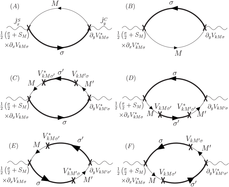
Figure 6: The diagrammatic expression for the term proportional to ${\partial}_{x}V_{{\bm{k}}M{\sigma}}{\partial}_{y}V_{{\bm{k}}M{\sigma}}$.

In the main text, we have calculated the term proportional to ${\partial}_{\mu}V{\partial}_{\nu}{\varepsilon}_{{\bm{k}}}$, and explained that it gives a dominant contribution to the SHC. In this appendix, we derive the SHC given by ${\partial}_{x}V_{{\bm{k}}}{\partial}_{y}V_{{\bm{k}}}$, and show that it is very small and negligible. In this case, to perform the $M,{\sigma}$-summations, we use the following relations:

$$\sum_{M,{\sigma}}\frac{1}{2}\left(\frac{{\sigma}}{2}-\frac{M}{7}\right)\frac{{\partial}V_{{\bm{k}}M{\sigma}}}{{\partial}k_{x}}\frac{{\partial}V_{{\bm{k}}M{\sigma}}^{\ast}}{{\partial}k_{y}}=i\frac{12}{7}\cos^{2}{\theta}\frac{1}{k^{2}}|V_{f}|^{2},{}$$

$$\sum_{M,M^{\prime},{\sigma},{\sigma}^{\prime}}\frac{1}{2}\left(\frac{{\sigma}}{2}-\frac{M}{7}\right)\frac{{\partial}V_{{\bm{k}}M{\sigma}}}{{\partial}k_{x}}V^{\ast}_{{\bm{k}}M{\sigma}^{\prime}}V_{{\bm{k}}M^{\prime}{\sigma}^{\prime}}\frac{{\partial}V^{\ast}_{{\bm{k}}M^{\prime}{\sigma}}}{{\partial}k_{y}}{}$$

$$=i\frac{16}{7}\cos^{2}{\theta}\frac{1}{k^{2}}|V_{f}|^{4},{}$$

$$\sum_{M,M^{\prime},{\sigma},{\sigma}^{\prime}}\frac{1}{2}\left(\frac{{\sigma}}{2}-\frac{M}{7}\right)\frac{{\partial}V_{{\bm{k}}M{\sigma}}}{{\partial}k_{x}}V^{\ast}_{{\bm{k}}M{\sigma}^{\prime}}V^{\ast}_{{\bm{k}}M^{\prime}{\sigma}}\frac{{\partial}V_{{\bm{k}}M^{\prime}{\sigma}^{\prime}}}{{\partial}k_{y}}{}$$

$$=-i\frac{16}{7}\cos^{2}{\theta}\frac{1}{k^{2}}|V_{f}|^{4}.$$ (51)

Here, we first perform the calculation for the Fermi surface term. By using the above relationship shown in eqs. (51), the SHC given by (A)-(D) in Fig. 6 is given by

$$\sigma_{\rm SH}^{I(A-D)} = \frac{e}{2\pi}\frac{8}{7}\sum_{{\bm{k}}}\frac{1}{k^{2}}|V_{f}|^{2}\text{Im}\left\{G^{fR}(0)G^{cA}(0)\right\}$$

$$+ \frac{e}{2\pi}\frac{64}{21}\sum_{{\bm{k}}}\frac{1}{k^{2}}|V_{f}|^{4}\text{Re}G^{fR}(0)\text{Im}G^{fR}(0)|G^{c}(0)|^{2}.{}$$

The diagrammatic expressions for eqs. (B) and (B) are respectively given by (A) and (B), and (C) and (D) in Fig. 6. The contributions from the diagrams (E) and (F) turn out to cancel out.

When ${\gamma}$ is small, we obtain a following relationship:

$$\text{Im}\left\{G^{fR}(0)G^{cA}(0)\right\}\approx\frac{\pi\delta(\mu-E_{{\bm{k}}})}{\mu-E^{f}},$$ (54)

$$\text{Re}G^{fR}(0)\text{Im}G^{fR}(0)|G^{c}(0)|^{2}\approx-\frac{1}{|V_{f}|^{2}}\frac{\pi\delta(\mu-E_{{\bm{k}}})}{\mu-E^{f}}.{}$$

Substituting the above equations into eqs. (B) and (B), and performing the ${\bm{k}}$-summation, we obtain

$$\sigma_{\rm SH}^{I} = \frac{e}{2\pi a}\frac{10}{21}\alpha N_{FS},$$ (56)

where $\alpha$ is defined by $|\mu-{\varepsilon}_{k_{F}}|=\alpha{\varepsilon}_{k_{F}}$.

In a similar way, we calculate $\sigma_{\rm SH}^{IIa}$ and $\sigma_{\rm SH}^{IIb}$. After performing the $M,\sigma$-summations using eq. (51), we obtain the following expression of the Fermi sea term for (A)-(D) in Fig. 6:

$$\sigma_{\rm SH}^{II(A-D)} =-\frac{e}{4\pi}\frac{48}{21}\sum_{{\bm{k}}}\frac{1}{k^{2}}|V_{f}|^{2}\text{Im}\left\{\int^{0}_{-\infty}d{\omega}\frac{{\partial}G^{fR}({\omega})}{{\partial}{\omega}}\cdot G^{cR}({\omega})-G^{fR}({\omega})\frac{{\partial}G^{cR}({\omega})}{{\partial}{\omega}}\right\}$$ (58)

$$-\frac{e}{2\pi a}\frac{128}{21}\sum_{{\bm{k}}}\frac{1}{k^{2}}|V_{f}|^{4}\text{Im}\left\{\int^{0}_{-\infty}d{\omega}\frac{{\partial}G^{fR}({\omega})}{{\partial}{\omega}}\cdot G^{fR}({\omega})\cdot\left(G^{cR}({\omega})\right)^{2}\right\}.$$

As explained in section III.2, after performing ${\omega}$-integration, above expressions are rewritten as follows for small $\gamma$:

$$\sigma_{\rm SH}^{IIa(A-D)} = \frac{e}{2\pi}\frac{24\pi}{21}\sum_{{\bm{k}}}\frac{1}{k^{2}}\frac{|V_{f}|^{2}}{E^{+}_{{\bm{k}}}-E^{-}_{{\bm{k}}}}\delta(\mu-E^{-}_{{\bm{k}}})-\frac{e}{2\pi}\frac{64\pi}{21}\sum_{{\bm{k}}}\frac{1}{k^{2}}\frac{|V_{f}|^{4}}{(E^{f}-E^{-}_{{\bm{k}}})(E^{+}_{{\bm{k}}}-E^{-}_{{\bm{k}}})^{2}}\delta(\mu-E^{-}_{{\bm{k}}}),{}$$

$$\sigma_{\rm SH}^{IIb(A-D)} = -\frac{e}{2\pi}\frac{48\pi}{21}\sum_{{\bm{k}}}\frac{1}{k^{2}}\frac{|V_{f}|^{2}}{(E^{+}_{{\bm{k}}}-E^{-}_{{\bm{k}}})(E^{f}-E^{-}_{{\bm{k}}})}\theta(\mu-E^{-}_{{\bm{k}}}){}$$

$$+\frac{e}{2\pi}\frac{64\pi}{21}\sum_{{\bm{k}}}\frac{1}{k^{2}}|V_{f}|^{4}\theta(\mu-E^{-}_{{\bm{k}}})\left[\frac{1}{(E^{f}-E^{-}_{{\bm{k}}})(E^{+}_{{\bm{k}}}-E^{-}_{{\bm{k}}})^{2}}+\frac{2}{(E^{f}-E^{-}_{{\bm{k}}})(E^{+}_{{\bm{k}}}-E^{-}_{{\bm{k}}})^{3}}\right].{}$$

Performing the ${\bm{k}}$-summations in eq. (LABEL:eq:IIa-bk), and as a result, we obtain the following expressions for $\sigma_{\rm SH}^{IIa}$:

$$\sigma_{\rm SH}^{IIa(A-D)} = \frac{e}{2\pi a}\Lambda_{k_{F}}\left[\frac{2}{7}\beta-\frac{16}{21}\alpha\right]N_{FS},$$ (61)

where $\beta$ is defined by $|E^{+}_{k_{F}}-\mu|=\beta{\varepsilon}_{k_{F}}$. As recognized in Fig. 1, the relation $\alpha\approx\beta\sim\frac{1}{2}$ is satisfied since $E^{+}_{k_{F}}\approx{\varepsilon}_{k_{F}}$ is satisfied in the present model. Since the relation $\Lambda_{k_{F}}=1+O((\Delta/V_{f})^{2})$ holds well as discussed in ref. III.2, $\sigma_{\rm SH}^{IIa}$ is given by

$$\sigma_{\rm SH}^{IIa(A-D)} = -\frac{e}{2\pi a}\frac{10}{21}N_{FS}\alpha.$$ (62)

To perform ${\bm{k}}$-summations in eq. (LABEL:eq:IIb-bk), we use the following approximation: $\displaystyle\sum_{{\bm{k}}}\frac{1}{k^{2}}\approx N(0)\frac{1}{k_{F}^{2}}\int d{\varepsilon}_{{\bm{k}}}$. Then, $\sigma_{\rm SH}^{IIb}$ is given by

$$\sigma_{\rm SH}^{IIb} = -\frac{e}{2\pi a}\left[\left\{-\frac{1}{14}+\frac{1}{21}\right\}\alpha+O\left(\frac{\Delta}{|V_{k_{F}}|}\right)\right]N_{FS}{}$$ (63)

$$= -\frac{e}{2\pi a}\frac{1}{42}N_{FS}\alpha.$$

Finally, we obtain the final expressions for $\sigma_{\rm SH}^{I},\sigma_{\rm SH}^{IIa}$, and $\sigma_{\rm SH}^{IIb}$ are given by the summations of eqs. (25) and (56), eqs. (37) and (61), and eqs. (38) and (63), respectively.

$$\sigma_{\rm SH}^{I-\rm{tot}} = -\frac{e}{2\pi a}\left(\frac{26}{21}-\frac{10}{21}\alpha\right)N_{FS},$$ (64)

$$\sigma_{\rm SH}^{IIa-\rm{tot}} = \frac{e}{2\pi a}\left(\frac{26}{21}-\frac{10}{21}\alpha\right)N_{FS},$$ (65)

$$\sigma_{\rm SH}^{IIb-\rm{tot}} = -\frac{e}{2\pi a}\left(\frac{26}{21}+\frac{1}{42}\alpha\right)N_{FS}.$$ (66)

Here in eqs. (64) -(66), the terms that is proportional to $\alpha$ is given in Fig. 6. In total, the SHC is given as

$$\sigma_{\rm SH}^{\rm{tot}}=-\frac{e}{2\pi a}\left(\frac{26}{21}+\frac{1}{42}\alpha\right)N_{\rm{FS}}.$$ (67)

In eq. (67), the factor ${26}/{21}$ and $\alpha/42$ in the bracket come from the terms with ${\partial}_{\mu}V_{{\bm{k}}}{\partial}_{\nu}{\varepsilon}_{{\bm{k}}}$ and the terms with ${\partial}_{\mu}V_{{\bm{k}}}{\partial}_{\nu}V_{{\bm{k}}}$, respectively. Since $\alpha\sim 1/2$, the terms proportional to ${\partial}_{\mu}V_{{\bm{k}}}{\partial}_{\nu}{\varepsilon}_{{\bm{k}}}$ shown in Fig. 4 gives a dominant contribution.

References

(1)
S. Murakami, N. Nagaosa and S.C. Zhang,
Phys. Rev. B 69 (2004) 235206.
(2)
J. Sinova, D. Culcer, Q. Niu, N. A. Sinitsyn, T. Jungwirth, and A. H. MacDonald,
Phys. Rev. Lett. 92 (2004) 126603.
(3)
J. I. Inoue, G. E. W. Bauer, and L. W. Molenkamp,
Phys. Rev. B70 (2004) 041303(R).
(4)
E. I. Rashba, Phys. Rev. B 70, 201309(R) (2004).
(5)
R. Raimondi and P. Schwab, Phys. Rev. B 71, 033311 (2005).
(6)
E. Saitoh, M. Ueda, H. Miyajima and G. Tatara,
Appl. Phys. Lett. 88 (2006) 182509.
(7)
S. O. Valenzuela and M. Tinkham,
Nature 442 (2006) 176.
(8)
N.P. Stern, S. Ghosh, G. Xiang, M. Zhu, N. Samarth, and D. D. Awschalom,
Phys. Rev. Lett. 97 (2006) 126603.
(9)
T. Kimura, Y. Otani, T. Sato, S. Takahashi, and S. Maekawa,
Phys. Rev. Lett. 98 (2007) 156601;
L. Vila , T. Kimura, and Y. C. Otani,
Phys. Rev. Lett. 99, 226604 (2007);
Y. Otani et al., (unpublished)
(10)
H. Kontani, T. Tanaka, D.S. Hirashima, K. Yamada, and J. Inoue:
Phys. Rev. Lett. 100, 096601 (2008).
(11)
H. Kontani, M. Naito, D.S. Hirashima, K. Yamada, and J. Inoue:
J. Phys. Soc. Jpn. 76 (2007) No.10.
(12)
G. Y. Guo, S. Murakami, T.-W. Chen, and N. Nagaosa, Phys. Rev. Lett. 100, 096401 (2008).
(13)
T. Tanaka, H. Kontani, M. Naito, T. Naito, D. S. Hirashima, K. Yamada, and J. Inoue,
Phys. Rev. B 77, 165117 (2008).
(14)
R. Karplus and J. M. Luttinger, Phys. Rev. 95, 1154 (1954).
(15)
H. Kontani, T. Tanaka, D. S. Hirashima, K. Yamada, and J. Inoue,
Phys. Rev. Lett. 102, 016601 (2009).
(16)
T. Namiki, H. Sato, H. Sugawara, Y. Aoki, R. Settai, and Y. Onuki, J. Phys. Soc. Jpn. 76 (2007) 054708.
(17)
A. Otop, S. Süllow, M. B. Maple, A. Weber, E. W. Scheidt, T. J. Gortenmulder, J. A. Mydosh, Phys. Rev. B 72 (2005) 024457.
(18)
S. Süllow, I. Maksimov, A. Otop, F. J. Litterst, A. Perucchi, L. Degiorgi, and J. A. Mydosh, Phys. Rev. Lett. 93 (2004) 266602.
(19)
T. Hiraoka, T. Sada, T. Takabatake and H. Fujii, Physica B 186-188 703 (1993).
(20)
H. Kontani and K. Yamada, J. Phys. Soc. Jpn. 63, 2627 (1994).
(21)
H. Shishido, T. Shibauchi, K. Yasu, T. Kato, H. Kontani, T. Terashima,
and Y. Matsuda, Science 327, 980 (2010).
(22)
T. Tanaka and H. Kontani, New J. Phys. 11 013023 (2009).
(23)
H. Kontani, and K. Yamada,
J. Phys. Soc. Jpn. 65 (1996) 172;
H. Kontani, and K. Yamada,
J. Phys. Soc. Jpn. 66 (1997) 2232.
(24)
H. Kontani, J. Phys. Soc. Jpn. 73, 515 (2004);
N. Tsujii, H. Kontani, and K. Yoshimura,
Phys. Rev. Lett. 94 (2005) 057201.
(25)
H. Kontani, M. Miyazawa, and K. Yamada,
J. Phys. Soc. Jpn. 66 (1997) 2252.
(26)
P. Streda: J. Phys. C: Solid State Phys. 15 (1982) L717.
(27)
H. Kontani, T. Tanaka, and K. Yamada,
Phys. Rev. B 75 184416 (2007).
(28)
M. C. Gutzwiller, Phys. Rev. 137 A1762 (1965).
(29)
T. M. Rice and K. Ueda, Phys. Rev. Lett. 55 995 (1985);
T. M. Rice and K. Ueda, Phys. Rev. B 34 6420 (1986).
(30)
H. Kontani, Rep. Prog. Phys. 71 (2008) 026501.