The Mass of HD 38529c from Hubble Space Telescope Astrometry and High-Precision Radial Velocities

Abstract

Hubble Space Telescope (HST ) Fine Guidance Sensor astrometric observations of the G4 IV star HD 38529 are combined with the results of the analysis of extensive ground-based radial velocity data to determine the mass of the outermost of two previously known companions. Our new radial velocities obtained with the Hobby-Eberly Telescope and velocities from the Carnegie-California group now span over eleven years. With these data we obtain improved RV orbital elements for both the inner companion, HD 38529b and the outer companion, HD 38529c. We identify a rotational period of HD 38529 (P${}_{rot}=31.65\pm 0.17^{d}$) with FGS photometry. The inferred star spot fraction is consistent with the remaining scatter in velocities being caused by spot-related stellar activity. We then model the combined astrometric and RV measurements to obtain the parallax, proper motion, perturbation period, perturbation inclination, and perturbation size due to HD 38529c. For HD 38529c we find P = 2136.1 $\pm$ 0.3 d, perturbation semi-major axis $\alpha=1.05\pm 0.06$ mas, and inclination $i$ = 48.3$\fdg$0 $\pm$ 4$\fdg$0. Assuming a primary mass $M_{*}=1.48M_{\sun}$, we obtain a companion mass ${\it M}_{c}=17.6^{+1.5}_{-1.2}{\it M}_{Jup}$, $3\sigma$ above a 13 M${}_{\rm Jup}~{}$deuterium burning, brown dwarf lower limit. Dynamical simulations incorporating this accurate mass for HD 38529c indicate that a near-Saturn mass planet could exist between the two known companions. We find weak evidence of an additional low amplitude signal that can be modeled as a planetary-mass ($\sim$0.17M_Jup) companion at P$\sim 194$ days. Including this component in our modeling lowers the error of the mass determined for HD 38529c. Additional observations (radial velocities and/or Gaia astrometry) are required to validate an interpretation of HD 38529d as a planetary-mass companion. If confirmed, the resulting HD 38529 planetary system may be an example of a “Packed Planetary System”.

1 Introduction

HD 38529(= HIP 27253 = HR 1988 = PLX 1320) hosts two known companions discovered by high-precision radial velocity (RV) monitoring (Fischer et al., 2001, 2003; Wright et al., 2009). Previously published periods were P_b=14.31^d and P${}_{c}=2146^{d}$ with minimum masses $M_{b}sini=0.85$M${}_{\rm Jup}~{}$and $M_{c}sini=13.1$M_Jup, the latter right above the currently accepted brown dwarf mass limit. A predicted minimum perturbation for the outermost companion, HD 38529c, $\alpha_{c}=0.8$ millisecond of arc (mas), motivated us to obtain millisecond of arc per-observation precision astrometry with HST with which to determine its true mass (not the minimum mass, $M_{c}sini$). These astrometric data now span 3.25 years.

In the early phases of our project Reffert & Quirrenbach (2006) derived an estimate of the mass of HD 38529c from Hipparcos, obtaining ${\it M}_{c}=38^{+36}_{-19}$ M_Jup, well within the brown dwarf ’desert’. Recent comparisons of FGS astrometry with Hipparcos, e.g. van Leeuwen et al. (2007), suggest that we should obtain a more precise and accurate mass for HD 38529c. Our mass is derived from combined astrometric and RV data, continuing a series presenting accurate masses of planetary, brown dwarf, and non-planetary companions to nearby stars. Previous results include the mass of Gl 876b (Benedict et al., 2002a), of $\rho^{1}$ Cancri d (McArthur et al., 2004), $\epsilon$ Eri b (Benedict et al., 2006), HD 33636B (Bean et al., 2007), and HD 136118 b (Martioli et al., 2010).

HD 38529 is a metal-rich G4 IV star at a distance of about 40 pc. The star lies in the ’Hertzsprung Gap’ (Murray & Chaboyer 2002), a region typically traversed very quickly as a star evolves from dwarf to giant. Baines et al. (2008b) have measured a radius. HD 38529 also has a small IR excess found by Moro-Martín et al. (2007) with Spitzer and interpreted as a Kuiper Belt at 20–50 AU from the primary. Stellar parameters are summarized in Table 1.

In Section 2 we model RV data from four sources, obtaining orbital parameters for both HD 38529b and HD 38529c. We also discuss and identify RV noise sources. In Section 3 we present the results of our combined astrometry/RV modeling, concentrating on HD 38529c. We briefly discuss the quality of our astrometric results as determined by residuals, and derive an absolute parallax and relative proper motion for HD 38529, those nuisance parameters that must be removed to determine the perturbation parameters for the perturbation due to component c. Simultaneously we derive the astrometric orbital parameters. These, combined with an estimate of the mass of HD 38529, provide a mass for HD 38529c. Section 4 contains the results of searches for additional components, limiting the possible masses and periods of such companions. In Section 5 we discuss possible identification of an RV signal that remained after modeling components b and c. We discuss our results and summarize our conclusions in Section 6.

2 Radial Velocities

2.1 RV Orbits

We first model RV data, a significant fraction of which comes from the Hobby-Eberly Telescope (HET). Measurements from the California-Carnegie exoplanet research group (Wright et al., 2009) and a few from the McDonald Harlan J Smith telescope (Wittenmyer et al., 2009) were also included. The California-Carnegie data were particularly valuable, increasing the time span from four to over eleven years. Our astrometry covers a little only 70% of the orbit of HD 38529c, and in the absence of a multi-period span of radial velocities, would not be sufficient to establish accurate perturbation elements, particularly period, eccentricity, and periastron passage. All RV sources are listed in Table 2, along with the RMS of the residuals to the combined orbital fits described below. The errors for all published RV and our new HET RV have been modified by adding in quadrature the expected RV jitter from stellar activity determined in Section 2.2.

All the radial velocities were obtained using I₂ cell techniques. The HET data were obtained with the HET High-resolution Spectrograph (HRS), described in Tull (1998) and processed with the I₂ pipeline described in Bean et al. (2007), utilizing robust estimation to combine the all velocities from the individual chunks. Typically three HET observations are secured within 10–15 minutes. These are combined using robust estimation to form normal points for each night. The HET normal points and associated errors are listed in Table 3.

Combining RV observations from different sources is possible in the modeling environment we use. GaussFit Jefferys et al. (1988) has the capability to simultaneously solve for many separate velocity offsets (because velocities from different sources are relative, having differing zero points), along with the other orbital parameters. Relative offsets ($\gamma$) and associated errors are listed in Table 11.

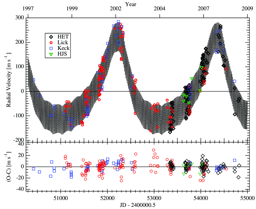
Figure 1: RV measurements of HD 38529 from sources as indicated in the legend (and identified in Table 2). The line is the velocity predicted from the orbital parameters (Table 11) derived in the combined solution. Residuals (RV observed minus RV calculated from the orbit) are plotted at bottom.

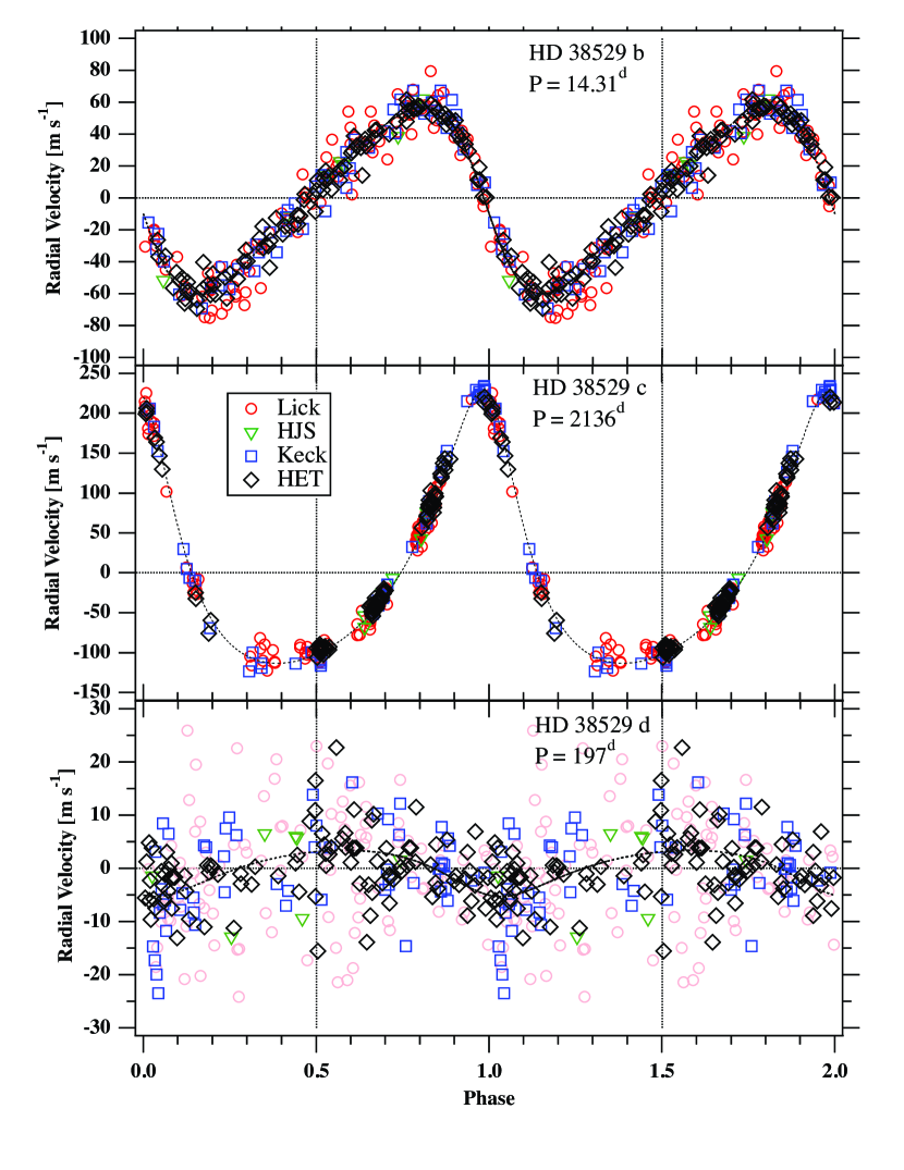
Figure 2: RV measurements of HD 38529 from sources as indicated in the legend (and identified in Table 2) phased to the orbital periods determined from a combined solution including astrometry and RV (Section 3.5). The dashed line is the velocity predicted from the orbital parameters (Table 11) derived in the combined solution.

Orbital parameters derived from a combination of HET, HJS, Lick, and Keck radial velocities and HST  astrometry will be provided in Section 3.5. Figure 1 shows the entire span of data along with the best fit multiple-Keplerian orbit. We note that there is sufficient bowing in the residuals to justify continued low-cadence RV monitoring, particularly given the prediction of Moro-Martín et al. (2007) of dynamical stability for planets with periods as short as $\sim 70$y. Subtracting in turn the signature of first one, then the other known companion from the original velocity data we obtain the component b and c RV orbits shown in Figure 2, each phased to the relevant periods. Re-iterating, all RV fits were modeled simultaneously with the astrometry.

Compared to the typical perturbation RV curve (e.g. Hatzes et al. 2005, McArthur et al. 2004, Cochran et al. 2004), our original orbits for components b and c exhibited significant scatter, much due to the identified stellar noise source discussed in Section 2.2 below. Periodogram analysis of RV residuals to simultaneous fits of components b and c indicated a significant peak with a period near 197 days. The existence of the signal is fairly secure. A bootstrap analysis carried out by randomly shuffling the RV residual values 200,000 times (keeping the times fixed), and determining if the random data periodogram had peaks higher than the real data periodogram in the frequency range $0<\nu<0.02~{}{\rm day}^{-1}$, yielded a false alarm probability, FAP =$5\times 10^{-4}$. This motivated the addition of a third Keplerian component, resulting in the fit shown in the bottom panel of Figure 2. Even though the amplitude of this signal is about that expected from stellar noise, including this component (five additional parameters) in the combined modeling improved both the reduced $\chi^{2}$, and the RMS scatter as shown in Table 2. Identification of the cause of the signal will be discussed further in Section 5.

2.2 Stellar Rotation and the RV Noise Level

There are a number of sources of RV noise intrinsic to HD 38529: pulsations and velocity perturbations introduced by star spots and/or plages. The velocity effects caused by the latter two are modulated by stellar rotation. Valenti & Fischer (2005) measure a rotation of HD 38529, V${}_{rot}\,sin\,i=3.5\pm 0.5$km s^-1 . HD 38529 is subgiant star, evolving towards the giant branch of the Hertszprung-Russell diagram, and is expected to have a higher level of pulsational activity than a main sequence star (Hatzes & Zechmeister, 2008). The pulsational amplitude can be estimated using the scaling relationship of Kjeldsen & Bedding (1995) $V_{amp}=(L/L_{\sun})/(M/M_{\sun})\times 0.234$ m s^-1. The luminosity and mass of HD 38529 yield a pulsational amplitude of $\sim 1$ m s^-1, so this alone cannot account for the excess RV scatter.

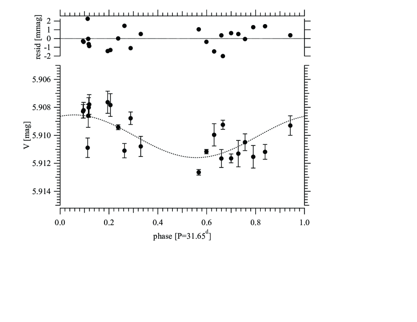
Figure 3: FGS photometry of HD 38529 phased to a period, P=31.65^d. HD 38529 intensities were flat-fielded with average counts from all astrometric reference stars observed during each observation set. Normal points are formed from the five observations of HD 38529 secured within each set. The zero-point is chosen so that the average V magnitude matches the SIMBAD value. The amplitude of the photometric variation is 0.15%. A periodogram of the flat field values shows no significant signals in the range $10<P<70^{d}$.

Several relationships between the amplitude of RV noise and the fraction of star spot coverage have been developed. Saar & Donahue (1997) obtain $A_{RV}=6.5\times v\,sin\,i\times f^{0.9}$, where $f$ is the spot filling factor in percent. Hatzes (2002) obtained $A_{RV}=(8.6v\,sin\,i-1.6)\times f^{0.9}$. We can estimate the spot filling factor from FGS photometry of HD 38529. The FGS has been shown to be a photometer precise at the 2 millimag (mmag) level (Benedict et al., 1998). We flat-fielded the HD 38529 FGS photometry, using an average of the counts from the astrometric reference stars listed in Table 5, and plotted it against time. Clearly not constant at a level ten times our internal precision, a Lomb-Scargle periodogram showed a significant period at P=31.6 days (FAP=$4.3\times 10^{-4}$). A sin wave fit to the photometry yielded P=$31.65\pm 0.17^{d}$ with an amplitude = 1.5 $\pm$ 0.2 mmag. Figure 3 is a plot of these photometric data phased to that period.

The Valenti & Fischer (2005) V${}_{rot}\,sin\,i=3.5$km s^-1 and a stellar radius from Baines et al. (2008b), R=2.44$\pm$0.22 R_☉, would predict a minimum P${}_{rot}=32\pm 5^{d}$. Interpreting the modulation period of 31.6 days as the stellar rotation period, we ascribe the photmetric variation (0.15%) to rotational modulation of star spots. The photometric amplitude suggests an RV noise level of 4–5 m s^-1. Taking the HET velocity RMS as closer to the true RV variation, we identify the remaining RV scatter as a combination of the three effects identified.

3 HST Astrometry

We used HST Fine Guidance Sensor 1r (FGS1r) to carry out our space-based astrometric observations. Nelan et al. (2007) provides a detailed overview of FGS1r as a science instrument. Benedict et al. (2002b, 2006) describe the FGS3 instrument’s astrometric capabilities along with the data acquisition and reduction strategies used in the present study. We use FGS1r for the present study because it provides superior fringes from which to obtain target and reference star positions (McArthur et al., 2002).

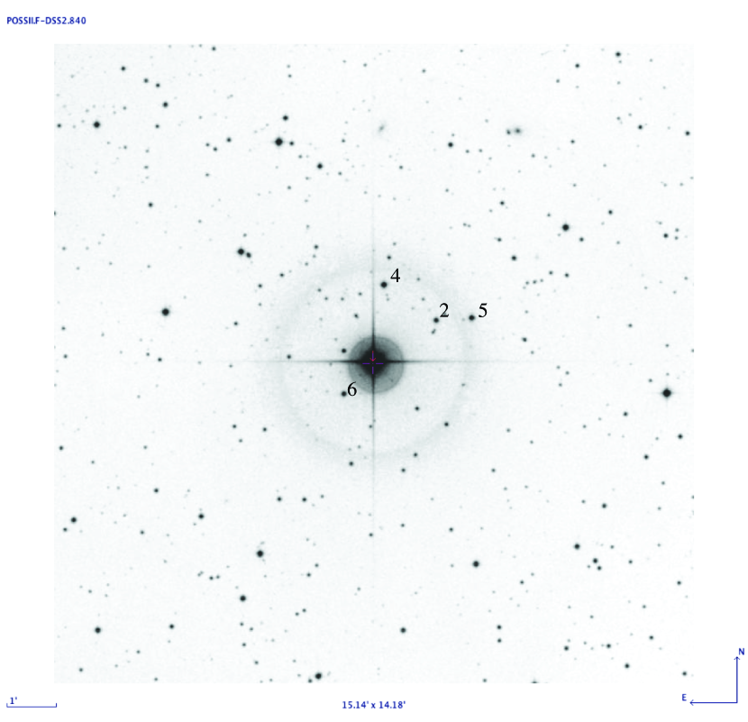
Figure 4: Positions of HD 38529 (center) and the astrometric reference stars identified in Table 5.

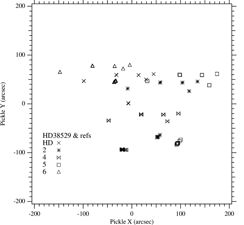
Figure 5: Positions of HD 38529 and astrometric reference stars in FGS1r ‘pickle’ coordinates. Due to two-gyro guiding constraints and guide star availability it was not possible to keep HD 38529 in the pickle center at each epoch.

HD 38529 is shown in Figure 4 along with the astrometric reference stars used in this study. Table 4 presents a log of HST FGS observations. Note the bunching of the observation sets, each ‘bunch’ with a time span less than a few days. Each set is tagged with the time of the first observation within each set. The field was observed at a very limited range of spacecraft roll values. As shown in Figure 5 HD 38529 had to be placed in different locations within the FGS1r FOV to accommodate the distribution of astrometric reference stars and to insure availability of guide stars required by the other two FGS units. Additionally, all observation sets suffered from observation timing constraints imposed by two-gyro guiding. Note that due to the extreme bunching of the epochs, we acquired effectively only five astrometric epochs. Also, we note that the last group of observation sets were a ‘bonus’. In November 2008 the only science instrument operating on HST was FGS1r. Consequently, we were able to acquire additional observation sets for a few of our prime science targets, including HD 38529. These recent data significantly lengthened the time span of our observations, hence, increased the precision with which the parallax and proper motion could be removed to determine the perturbation orbit of HD 38529. Once combined with an estimate of the mass of HD 38529, the perturbation size will provide the mass of the companion, HD 38529c.

3.1 HD 38529 Astrometric Reference Frame

The astrometric reference frame for HD 38529 consists of four stars. Any prior knowledge concerning these four stars eventually enters our modeling as observations with error, and yields the most accurate parallax and proper motion for the prime target, HD 38529. These periodic and non- periodic motions must be removed as accurately and precisely as possible to obtain the perturbation inclination and size caused by HD 38529c. Of particular value are independently measured proper motions. This particular prior knowledge comes from the UCAC3 catalog Zacharias et al. (2009). Figure 5 shows the distribution in FGS1r pickle coordinates of the 23 sets of four reference star measurements for the HD 38529 field. At each epoch we measured each reference stars 2 – 4 times, and HD 38529 five times.

3.2 Absolute Parallaxes for the Reference Stars

Because the parallax determined for HD 38529 is measured with respect to reference frame stars which have their own parallaxes, we must either apply a statistically- derived correction from relative to absolute parallax (van Altena et al., 1995, Yale Parallax Catalog, YPC95), adopt an independently derived parallax (e.g., Hipparcos), or estimate the absolute parallaxes of the reference frame stars. In principle, the colors, spectral type, and luminosity class of a star can be used to estimate the absolute magnitude, $M_{V}$, and $V$-band absorption, $A_{V}$. The absolute parallax for each reference star is then simply,

$$\pi_{\rm abs}=10^{-(V-M_{V}+5-A_{V})/5}$$ (1)

3.2.1 Reference Star Photometry and Spectroscopy

Our band passes for reference star photometry include: $BVRI$ photometry of the reference stars from the NMSU 1 m telescope located at Apache Point Observatory and JHK (from 2MASS). Table 7 lists the visible and infrared photometry for the HD 38529 reference stars. The spectra from which we estimated spectral type and luminosity class were obtained on 2009 December 9 using the RCSPEC on the Blanco 4 m telescope at CTIO. We used the KPGL1 grating to give a dispersion of 0.95 Å/pix. Classifications used a combination of template matching and line ratios. The spectral types for the higher S/N stars are within $\pm$1 subclass. Classifications for the lower S/N stars are $\pm$2 subclasses. Table 7 lists the spectral types and luminosity classes for our reference stars.

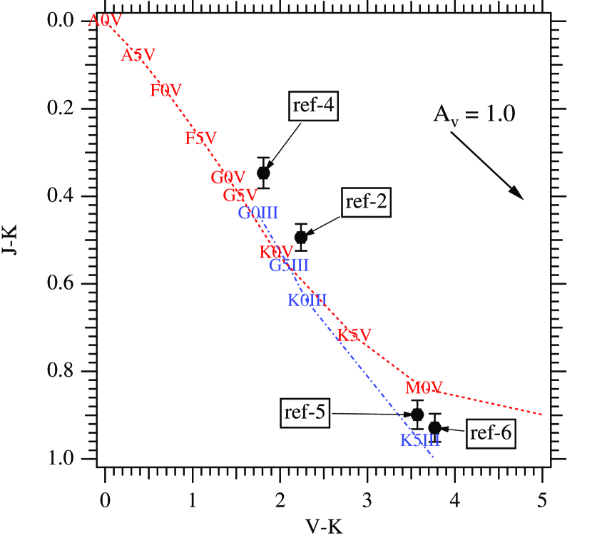
Figure 6: $(J-K)$ vs. $(V-K)$ color-color diagram for stars identified in Table 5 and Table 6. The dashed line is the locus of dwarf (luminosity class V) stars of various spectral types; the dot-dashed line is for giants (luminosity class III). The reddening vector indicates $A_{V}=1.0$ for the plotted color systems. Along this line of sight maximum extinction is $A_{V}$$\sim$ 2 (Schlegel et al., 1998).

Figure 6 contains a $(J-K)$ vs. $(V-K)$ color-color diagram of the reference stars. Schlegel et al. (1998) find an upper limit $A_{V}$$\sim$2 towards HD 38529, consistent with the absorptions we infer comparing spectra and photometry (Table 7).

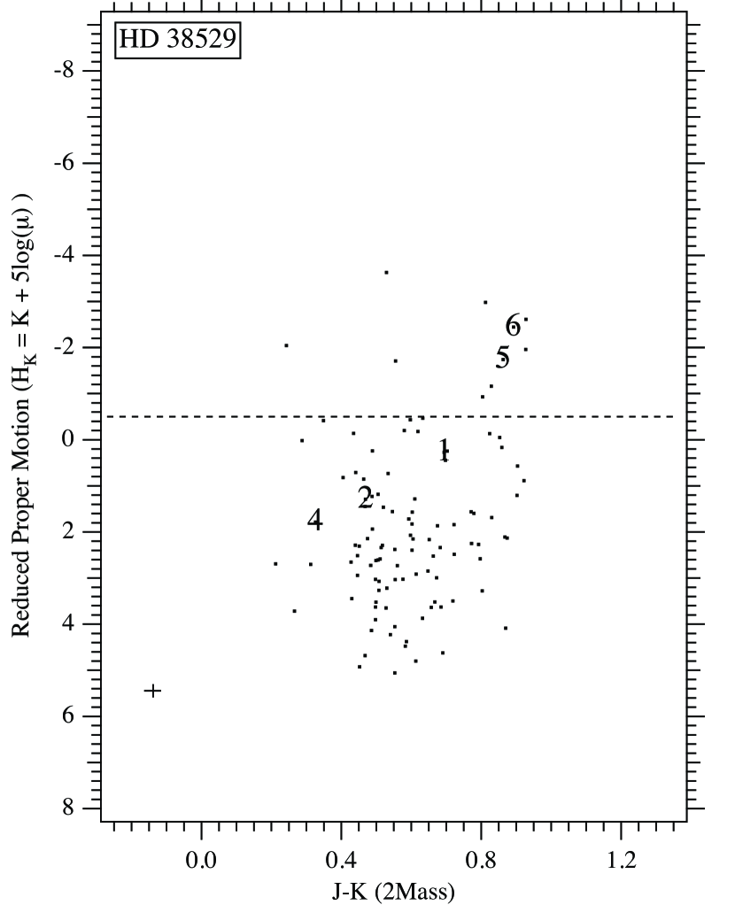
Figure 7: Reduced proper motion diagram for 107 stars in a 1/3° field centered on HD 38529. Star identifications are in Table 5. For a given spectral type, giants and sub-giants have more negative $H_{K}$ values and are redder than dwarfs in $(J-K)$. $H_{K}$ values are derived from proper motions in Table 9. The small cross at the lower left represents a typical $(J-K)$ error of 0.04 mag and $H_{K}$ error of 0.17 mag. Ref-5 and -6 are confirmed to have luminosity class III. HD 38529 (#1 in plot) is also intermediate (luminosity class IV) in this parameter space.

The derived absolute magnitudes are critically dependent on the assumed stellar luminosity, a parameter impossible to obtain for all but the latest type stars using only Figure 6. To confirm the luminosity classes obtained from classification spectra we abstract UCAC3 proper motions Zacharias et al. (2009) for a one-degree-square field centered on HD 38529, and then iteratively employ the technique of reduced proper motion (Yong & Lambert, 2003; Gould & Morgan, 2003) to discriminate between giants and dwarfs. The end result of this process is contained in Figure 7. Reference stars ref-5 and ref-6 are confirmed to have luminosity class III (giant).

3.2.2 Adopted Reference Frame Absolute Parallaxes

We derive absolute parallaxes by comparing our estimated spectral types and luminosity class to $M_{V}$ values from Cox (2000). Our adopted input errors for distance moduli, $(m-M)_{0}$, are 0.5 mag for all reference stars. Contributions to the error are uncertainties in $A_{V}$ and errors in $M_{V}$ due to uncertainties in color to spectral type mapping. All reference star absolute parallax estimates are listed in Table 7. Individually, no reference star absolute parallax is better determined than ${\sigma_{\pi}\over\pi}$ = 23%. The average input absolute parallax for the reference frame is $\langle\pi_{abs}\rangle=0.8$ mas. We compare this to the correction to absolute parallax discussed and presented in YPC95 (sec. 3.2, fig. 2). Entering YPC95, fig. 2, with the Galactic latitude of HD 38529, $b=-19\arcdeg$, and average magnitude for the reference frame, $\langle V_{\rm ref}\rangle=13.85$, we obtain a correction to absolute of 1.2 mas, consistent with our derived correction. As always (Benedict et al., 2002c, b, a; McArthur et al., 2004; Soderblom et al., 2005; Benedict et al., 2006, 2007), rather than apply a model-dependent correction to absolute parallax, we introduce our spectrophotometrically-estimated reference star parallaxes into our reduction model as observations with error.

3.3 The Astrometric Model

The HD 38529 reference frame contains only four stars. From positional measurements we determine the scale, rotation, and offset “plate constants” relative to an arbitrarily adopted constraint epoch for each observation set. As for all our previous astrometric analyses, we employ GaussFit (Jefferys et al. 1988) to minimize $\chi^{2}$. The solved equations of condition for the HD 38529  field are:

$$x^{\prime}=x+lc_{x}(\it B-V)-\Delta XF_{x}$$ (2)

$$y^{\prime}=y+lc_{y}(\it B-V)-\Delta XF_{y}$$ (3)

$$\xi=Ax^{\prime}+By^{\prime}+C-\mu_{\alpha}\Delta t-P_{\alpha}\pi-ORBIT_{x}$$ (4)

$$\eta=Dx^{\prime}+Ey^{\prime}+F-\mu_{\delta}\Delta t-P_{\delta}\pi-ORBIT_{y}$$ (5)

for FGS1r data. Identifying terms, $\it x$ and $\it y$ are the measured coordinates from HST; $(B-V)$ is the Johnson $(B-V)$ color of each star; and $\it lc_{x}$ and $\it lc_{y}$ are the lateral color corrections, applied only to FGS1r data. Here $\Delta XF_{x}$ and $\Delta XF_{y}$are cross filter corrections (see Benedict et al. 2002b) in $\it x$ and $\it y$, applied to the observations of HD 38529. $A$, $B$, $D$ and $E$ are scale- and rotation plate constants, $C$ and $F$ are offsets; $\mu_{\alpha}$ and $\mu_{\delta}$ are proper motions; $\Delta t$ is the epoch difference from the constraint epoch; $P_{\alpha}$ and $P_{\delta}$ are parallax factors; and $\it\pi$ is the parallax. We obtain the parallax factors from a JPL Earth orbit predictor (Standish 1990), upgraded to version DE405. Orientation to the sky for the FGS1r data is obtained from ground-based astrometry (2MASS Catalog) with uncertainties of $0\fdg 01$. $ORBIT_{x}$ and $ORBIT_{y}$ are functions (through Thiele-Innes constants, e.g., Heintz, 1978) of the traditional astrometric and RV orbital elements listed in Table 11.

3.4 Assessing Reference Frame Residuals

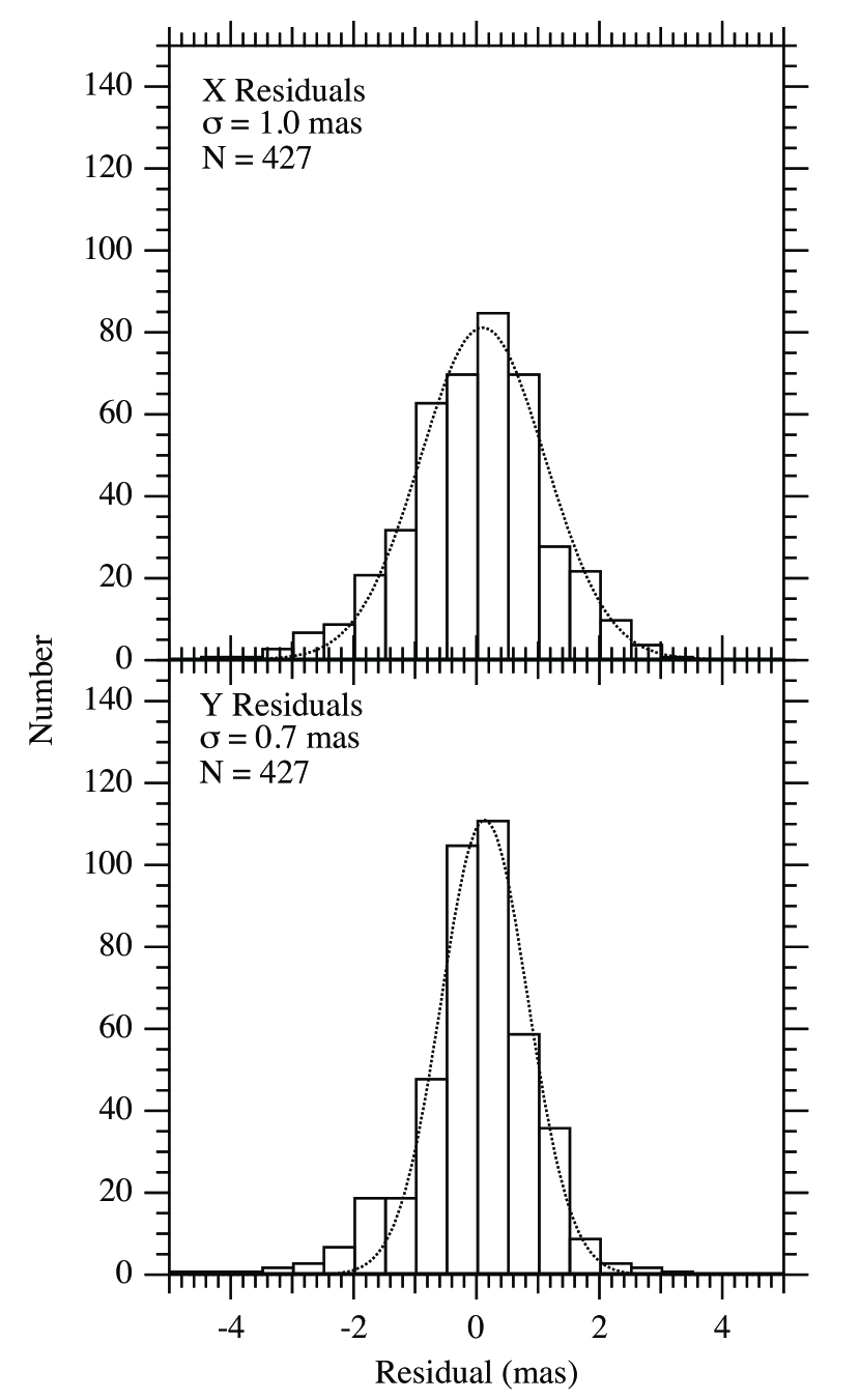
Figure 8: Histograms of x and y residuals obtained from modeling the FGS observations of HD 38529 and the FGS reference frame with equations 4 and 5. Distributions are fit with gaussians with standard deviations, $\sigma$, indicated in each panel.

The Optical Field Angle Distortion calibration (McArthur et al., 2002) reduces as-built HST telescope and FGS1r distortions with magnitude $\sim 1\arcsec$ to below 2 mas over much of the FGS1r field of regard. These data were calibrated with a revised OFAD generated by McArthur in 2007. From histograms of the FGS astrometric residuals (Figure 8) we conclude that we have obtained correction at the $\sim 1$ mas level. The reference frame ’catalogs’ from FGS1r in $\xi$ and $\eta$ standard coordinates (Table 8) were determined with $<\sigma_{\xi}>=0.15$ and $<\sigma_{\eta}>=0.15$ mas.

3.5 The Combined Orbital Model

We linearly combine unperturbed Keplerian orbit, simultaneously modelling the radial velocities and astrometry. The period (P), the epoch of passage through periastron in years (T), the eccentricity (e), and the angle in the plane of the true orbit between the line of nodes and the major axis ($\omega$), are the same for an orbit determined from RV or from astrometry. The remaining orbital elements come only from astrometry. We force a relationship between the astrometry and the RV through this constraint (Pourbaix & Jorissen, 2000)

$${{\alpha~{}sin~{}i\over\pi_{abs}}={PK(1-e^{2})^{1/2}\over 2\pi\times 4.7405}}$$ (6)

where quantities derived only from astrometry (parallax, $\pi_{abs}$, primary perturbation orbit size, $\alpha$, and inclination, $i$) are on the left, and quantities derivable from both (the period, $P$ and eccentricity, $e$), or radial velocities only (the RV amplitude of the primary, $K$), are on the right. In this case, given the fractional orbit coverage of the HD 38529c perturbation afforded by the astrometry, all right hand side quantities are dominated by the radial velocities.

For the parameters critical in determining the mass of HD 38529 we find a parallax, $\pi_{abs}=25.11\pm 0.19$ mas and a proper motion in RA of $-78.60\pm 0.15$ mas y^-1 and in DEC of $-141.96\pm 0.11$ mas y^-1. Table 10 compares values for the parallax and proper motion of HD 38529 from HST and both the original Hipparcos values and the recent Hipparcos re-reduction (van Leeuwen, 2007). We note satisfactory agreement for parallax and proper motion. Our precision and extended study duration have significantly improved the accuracy and precision of the parallax and proper motion of HD 38529.

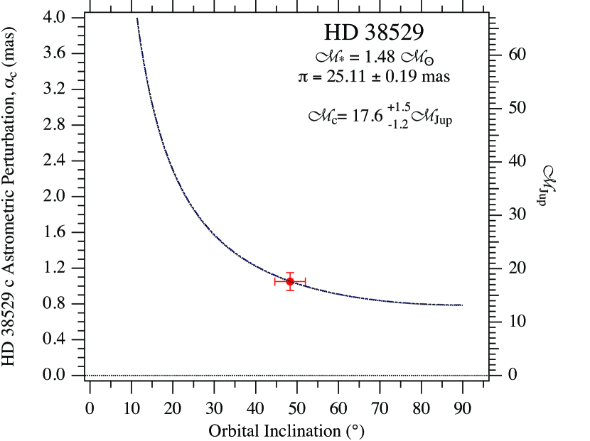
Figure 9: This curve relates perturbation size and inclination for the HD 38529c perturbation through the Pourbaix & Jorrisen (2000) relation (Equation 6). We use the curve as a ’prior’ in a quasi-bayesian sense. Our final values for the semimajor axis of the astrometric perturbation, $\alpha_{c}$, and inclination, $i_{c}$ are plotted with the formal errors.

We find a perturbation size, $\alpha_{c}=1.05\pm 0.06$ mas, and an inclination, $i$= 48$\fdg$3 $\pm$ 3$\fdg$7. These, and the other orbital elements are listed in Table 11 with 1-$\sigma$ errors. Figure 9 illustrates the Pourbaix and Jorrisen relation (Equation 6) between parameters obtained from astrometry (left-side) and radial velocities (right side) and our final estimates for $\alpha_{c}$ and $i$. In essence, our simultaneous solution uses the Figure 9 curve as a quasi-Bayesian prior, sliding along it until the astrometric and RV residuals are minimized. Gross deviations from the curve are minimized by the high precision of all of the right hand side terms in Equation 6 (Tables 10 and 11).

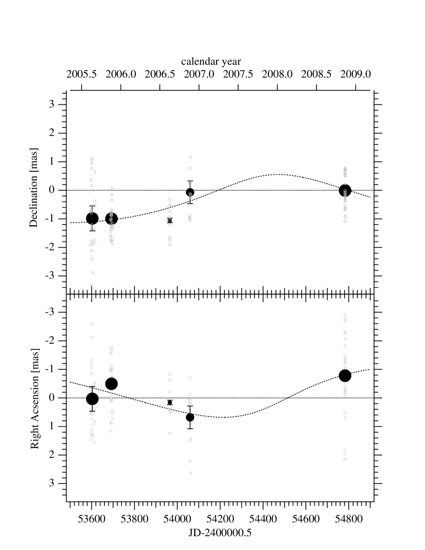
Figure 10: RA (bottom) and Dec (top) components of the perturbation orbit for HD 38529c as a function of time. The dashed line is the orbit described by the orbital elements found in Table 11. The small symbols are all the HD 38529 observation residuals to a model that does not contain orbital motion. The large symbols are normal points formed at each average epoch. Symbol size is proportional to the number of individual observations at each normal point epoch.

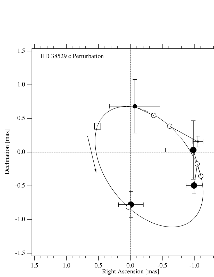
Figure 11: Perturbation orbit for HD 38529c. Elements are found in Table 11. Residual vectors are plotted, connecting each normal point residual to its predicted position (O) at each epoch of observation. Error bars indicate the positional 1-$\sigma$ normal point dispersion within each epoch. Normal point symbol size is proportional to the number of individual observations at each normal point epoch. The open square marks periastron passage, T₀=2013.68, and the arrow indicates the direction of perturbation motion.

At this stage we can assess the reality of the HD 38529c astrometric perturbation by plotting the astrometric residuals from a model that does not include a component c orbit. Figure 10 shows the RA and Dec components of the FGS residuals plotted as small symbols. We also plot normal points formed from those smallest symbols within each of the 23 data sets listed in Table 4. The largest symbols denote the final normal points formed for each of our (effectively) five epochs. Finally, each plot contains as a dashed line the RA and Dec components of the perturbation we find by including an orbit in our modeling. Finally, Figure 11 shows the perturbation on the sky with our normal points.

The planetary mass depends on the mass of the primary star, for which we have adopted $M_{*}=1.48M_{\sun}$ (Takeda et al., 2007). For that $M_{*}$ we find $M_{c}=17.6^{+1.5}_{-1.2}$M_Jup, a significant improvement over the Reffert & Quirrenbach (2006) estimate, ${\it M}_{c}=38^{+36}_{-19}$ M_Jup, but agreeing within the errors. HD 38529c is likely a brown dwarf, but only about 3-$\sigma$ from the ‘traditional’ planet-brown dwarf dividing line, 13M_Jup, the mass above which deuterium is thought to burn. In Table 11 the mass value, $M_{c}$, incorporates the present uncertainty in $M_{*}$. However, the dominant source of error is in the inclination estimate. Until HD 38529 c is directly detected, its radius is unknown. Comparing to the one known transiting brown dwarf, CoRot-Exo-3b (Deleuil et al., 2008), a radius of $R\sim 1R_{JUP}$ seems reasonable.

4 Limits on Additional Planets in the HD 38529 System

The existence of additional companions in the HD 38529 system is predicted by the “Packed Planetary Systems” hypothesis (Barnes & Raymond, 2004; Raymond & Barnes, 2005). Specifically those investigations identified the range of orbits in which an additional planet in between planets b and c would be stable. Having access to eleven years of HD 38529 RV observations permits a search for longer-period companions. Our velocity database, augmented by high-cadence ($\Delta$t often less than 2 days, Table 3) HET monitoring, supports an exploration for shorter-period companions. Additionally, a relatively precise actual mass for HD 38529c better informs any companion searches based on dynamical interaction.

We independently examined the possible dynamical stability of an additional planet in the system by performing long-term N-body integrations of the orbits of the known planets and test particles in a manner similar to (Barnes & Raymond, 2004). The orbital parameters of the known planets were taken to be those we have determined. Our advantage over previous stability investigations; the true mass of planet c was used. Planet b was assumed to be coplanar with planet c, and its mass was computed based on its minimum mass and the inclination of planet c. The test particles were initialized in orbits also coplanar with planet c, and with semimajor axes ranging from 0.01 to 10.0 AU. The spacing was linear in the logarithm of the semimajor axis and 301 test particles were used. Simulations were done using three different eccentricity values for the test particles: e=0.0, 0.3. and 0.7. All the the calculations were carried out using the “Hybrid” integrator in the Mercury code (Chambers, 1999). The simulations were performed over 10⁷ yr and the integration parameters were tuned so that the fractional energy error was $<10^{-4}$.

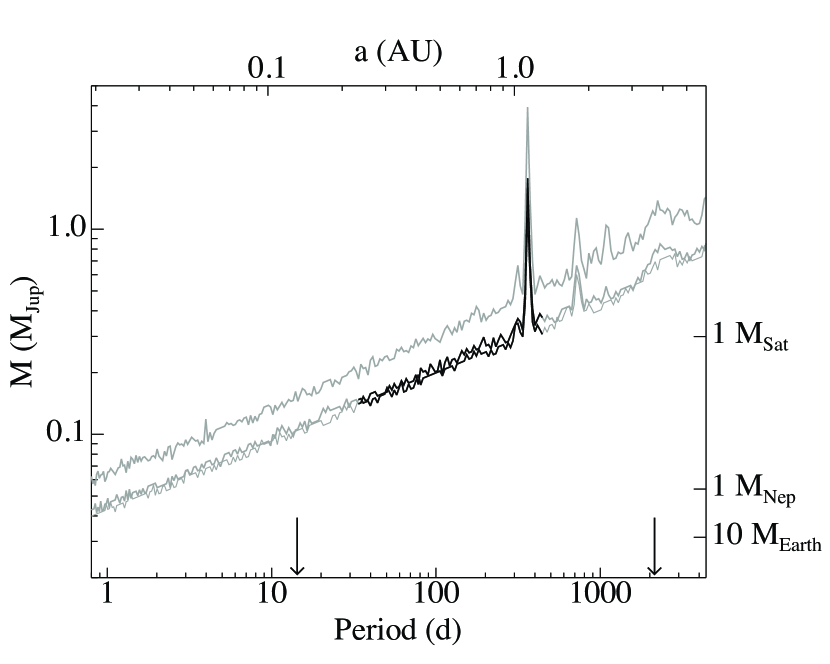
Figure 12: Results from the detection limit simulations converted to mass of a companion assuming coplanarity with HD 38529c. Values above the lines would have been detected in a periodogram analysis of the RV data. The different lines represent the different assumed eccentricity values (lower: e=0.0, middle: e=0.3, upper: e=0.7). The black and grey parts of the lines indicate regions where test particles in the long-term simulation were stable and unstable respectively. The arrows indicate the orbital periods of the known planets.

From these simulations we find that no additional planets would be stable over long timescales interior to planet b. Between planets b and c, we find that planets with eccentricities less than 0.3 would be stable over the semimajor axis range 0.23 – 1.32 AU (P = 33 – 455 days). Exterior to planet c, no additional planets would be stable in orbits with periods shorter than the time baseline of the RV observations. Additional planets with eccentricities of 0.7 would not be stable over the entire range considered. These results are illustrated in Figure 12, and are completely consistent with the results of Barnes & Raymond (2004).

5 Evidence for a Possible Tertiary, HD 38529d

We have previously mentioned (Section 2.1) a signal in the RV data residuals that remains after the signatures of components b and c are removed. An orbital fit to those residuals from the two component fit to HD 38529b and c is shown in the bottom panel of Figure 2 with the low-precision elements of this possible component d presented in Table 11. Table 12 contains the orbital elements from a solution in which only components b and c are modeled. While these astrometric elements closely agree with the three component solution in Table 11, the errors are larger. When HD 38529d is added to the model (adding 5 degrees of freedom, an increase of 1.5%) the $\chi^{2}$ of the RV fit drops by 13%, from 287 to 258. Comparing Tables 11 and 12, we see a similar reduction in the error in the mass of component c, the primary result of this study. HD 38529c remains a brown dwarf, whether or not component d is introduced.

We have explored sampling as a cause for the low-amplitude component d signal by performing power spectrum analysis of artificial RV generated from the component b and c orbits in Table 12, sampled on the dates of all the RV observations. There are no peaks at P=194 days. To test for a seasonal effect in our HET data, one that might introduce a variation at the period of the tentative component d, we first removed the the large-amplitude component b and c signals. We then combined the residuals containing the low amplitude signal of HD 38529d with the low amplitude signals found for HD 74156c (Bean et al., 2008) and HD 136118c (Martioli et al., 2010). The power spectrum of this aggregate should show seasonal fluctuations, if present. We saw nothing but expected signals (due to sampling) at 1/6, 1/2, and one year.

Both the study in Section 4 above and the packed planetary system hypothesis Raymond et al. (2009), allow this as a potential tertiary in the system. Furthermore, a stability analysis of the system, assuming all planets lie on the same plane as planet c, demonstrated the planet is stable, consistent with the results of Barnes & Raymond (2004). We performed this test with HNBody which accounts for any general relativistic precession of planet b. However, the amplitude of the HD 38529d signal is very small, $K\sim 5$m s^-1, at the level of expected stellar Doppler noise (Section 2.2). The higher-cadence HET data set which could most clearly identify this object, does not span enough time for an adequate fit to the longer period HD 38529c. An unconstrained fit of HET data alone will not be possible for several more years. Therefore, we advise caution in the use of the elements listed in Table 11 and in the adoption of this signal as unequivocal evidence of a component d. Confirmation will require additional high-cadence RV observations, and/or future astrometry. A minimum mass component d would generate a peak to peak astrometric signature of 52 microarcseconds, likely detectable by Gaia (Casertano et al., 2008).

6 Discussion and Conclusions

6.1 Discussion

Given the adopted Table 11 errors, HD 38529c is either one of the most massive exoplanets or one of the least massive brown dwarfs. We can compare our true mass to the (as of January 2010) 69 transiting exoplanetary systems, each also characterized by true mass, not $M\sin{\it i}~{}$. As shown in the useful Exoplanetary Encyclopedia (Schneider, 2009) only one companion (CoRoT-Exo-3 b, Deleuil et al. 2008) has a mass in excess of 13M_Jup. Whether this ’brown dwarf desert’ (Grether & Lineweaver, 2006) in the transiting sample is due to the difficulty of migrating high-mass companions (bringing them in close enough to increase the probability of transit), or to inefficiencies in gravitational instability formation is unknown.

The age of the host star, $\sim 3.3$ By, would suggest that HD 38529c has not yet cooled to an equilibrium temperature. An estimated temperature and self-luminosity for a 17M${}_{\rm Jup}~{}$object that is 3.3 By old can be found from the models of Hubbard et al. (2002). Those models predict that HD 38529c has an effective temperature, T${}_{eff}\simeq 400$K, and L=2.5e-7L_☉, about 20 times brighter than what we estimated using these same models for $\epsilon$ Eri b (Benedict et al., 2006). Unfortunately HD 38529 has about 16 times the intrinsic brightness of $\epsilon$ Eri, erasing any gain in contrast. We note that due to the eccentricity of the orbit, HD 38529c is actually within the present day habitable zone for a fraction of its orbit. As HD 38529 continues to evolve and brighten, the habitable zone will move outward and HD 38529c will be in that zone for some period of time.

If the inner known companion HD 38529b is a minimum mass exoplanetary object (assuming $M=Msini=0.8$M${}_{\rm Jup}~{}$), our 1 mas astrometric per-observation precision precludes detecting that 2 microsecond of arc signal. Invoking (with no good reason) coplanarity with HD 38529c similarly leaves us unable to detect HD 38529b. However, with the motivation of our previous result for HD 33636 (Bean et al., 2007), we can test whether or not HD 38529b is also stellar by establishing an upper limit from our astrometry. To produce a perturbation, $\alpha_{b}>0.2$ mas (a 3-$\sigma$ detection, given $\sigma_{\alpha}=0.06$ mas from Table 11), and the observed RV amplitude, K_b=59m s^-1, requires $M_{b}\sim 0.1M_{\sun}$ in an orbit inclined by less than 0$\fdg$5. Our limit is lower than that established with the CHARA interferometer (Baines et al., 2008a), who established a photometric upper limit of G5 V for the b component. While it might be possible to use 2MASS and SDSS (Ofek, 2008) photometry of this object to either confirm or eliminate a low-mass stellar companion by backing out a possible contribution from an M, L, or T dwarf, using their known photometric signatures (Hawley et al., 2002; Covey et al., 2007), we lack precise (1%) knowledge of the intrinsic photometric properties of a sub-giant star in the Hertzsprung gap with which to compare.

6.2 Conclusions

In summary, radial velocities from four sources, Lick and Keck (Wright et al., 2009), HJS/McDonald (Wittenmyer et al., 2009), and our new high-cadence series from the HET, were combined with HST  astrometry to provide improved orbital parameters for HD 38529b and HD 38529c. Rotational modulation of star spots with a period P=31.66$\pm$0.17^d produces 0.15% photometric variations, spot coverage sufficient to produce the observed residual RV variations. Our simultaneous modeling of radial velocities and over three years of HST FGS astrometry yields the signature of a perturbation due to the outermost known companion, HD 38529c. Applying the Pourbaix & Jorrisen constraint between astrometry and radial velocities, we obtain for the perturbing object HD 38529c a period, P = 2136.1 $\pm$ 0.3 d, inclination, $i$=48.3$\fdg$2 $\pm$ 3.7°, and perturbation semimajor axis, $\alpha_{c}=1.05\pm 0.06$ mas. Assuming for HD 38529 a stellar mass $M_{*}$ = 1.48$\pm$0.05$M_{\sun}$, we obtain a mass for HD 38529 c, $M_{b}$ = 17.6${}^{+1.5}_{-1.2}$M${}_{\rm Jup}~{}$, within the brown dwarf domain. Our independently determined parallax agrees within the errors with Hipparcos, and we find a close match in proper motion. Our HET radial velocities combined with others establish an upper limit of about one Saturn mass for possible companions in a dynamically stable range of companion-star separations, $0.2\leq a\leq 1.2$ AU. RV residuals to a model incorporating components b and c contain a signal with an amplitude equal to the RMS variation with a period, P$\sim 194^{d}$ and an inferred $a\sim 0.75$ AU. While dynamical simulations do not rule out interpretation as a planetary mass companion, the low S/N of the signal argues for confirmation.

Table 1: HD 38529 Stellar Parameters

Parameter	Value	Source
SpT	G4 IV	1, 9
Teff	5697 K	2
log g	3.94 $\pm$ 0.1	2
$[Fe/H]$	0.27 $\pm$ 0.05	2
age	3.28 $\pm$ 0.3 By	2
mass	1.48 $\pm$ 0.05 $M_{\sun}$	2
distance	40.0 $\pm$ 0.5 pc	3
R	2.44 $\pm$ 0.22$R_{\sun}$	4
v sin i	3.5 $\pm$ 0.5 km s-1	5
V	5.90 $\pm$ 0.03	6
K	4.255 $\pm$ 0.03	7
V-K	1.65 $\pm$ 0.04
i-z	0.06	8
g-r	0.55	8
r-i	0.15	8

¹Fischer et al. 2001, ²Takeda (2007) or Takeda et al. (2007), ³parallax from Table 10, ⁴Baines et al. (2008b), ⁵Valenti & Fischer (2005), ⁶SIMBAD, ⁷2MASS, ⁸Ofek (2008), ⁹Murray & Chaboyer (2002).

Table 2: The RV Data Sets

Data Set	Coverage	Nobs	RMS [m s-1]
			3C	2C
Lick	1998.79-2008.22	109	10.34	10.74
HJS	1995.72-1996.78	7	7.24	7.56
Keck	1996.92-2008.07	55	7.39	7.90
HET	2004.92-2008.98	313	5.75	5.92
	total	484

Table 3: HET RV Data

JD-2450000	RV (m/s)	$\pm$ error
3341.779899	-105.27	7.77
3341.898484	-118.43	7.25
3355.845730	-102.05	7.34
3357.859630	-105.27	7.48
3358.724097	-87.82	7.11
3359.729188	-82.07	8.70
3360.849520	-65.85	7.80
3365.817387	1.45	7.73
3367.812640	-20.41	9.48
3369.701315	-90.14	8.57
3371.684761	-107.83	8.90
3377.785833	-20.51	8.92
3379.675805	-3.53	6.78
3389.755622	-50.16	7.68
3390.763879	-35.52	7.46
3391.757235	-19.07	8.15
3392.750785	-5.45	7.11
3395.738803	2.78	6.97
3414.693834	-103.63	10.96
3416.683636	-74.10	8.61
3665.892690	64.01	4.74
3675.986919	6.80	5.07
3676.846929	21.68	5.48
3678.862452	42.80	5.63
3681.843596	51.51	5.06
3685.835951	-63.04	25.10
3685.837515	-57.70	5.16
3691.933851	27.17	5.07
3692.834053	39.74	5.00
3694.820769	63.79	5.48
3695.817331	61.75	5.81
3696.807526	47.54	4.91
3697.813712	8.53	5.32
3700.809061	-38.81	5.48
3708.894418	64.36	6.38
3709.886951	60.71	5.85
3711.767580	20.98	5.68
3712.875847	-26.85	7.10
3724.839770	60.73	6.27
3730.717661	-28.39	7.05
3731.708724	-18.87	6.85
3733.706335	16.30	6.90
3735.713861	48.56	6.86
3739.692156	48.28	6.40
3742.684910	-46.27	5.94
3751.775752	73.88	6.84
3752.761925	74.25	6.79
3753.773028	64.34	7.73
3754.760139	35.42	6.79
3755.751319	-9.88	6.38
3757.639021	-39.51	6.53
3758.754961	-29.76	6.22
3764.745400	62.37	6.78
3989.998171	88.56	5.09
4020.924198	141.62	5.36
4021.921835	158.20	5.52
4022.926094	164.55	8.27
4028.903039	75.06	5.75
4031.882076	104.25	5.64
4031.997118	111.67	5.86
4035.887008	164.27	6.09
4037.876174	185.49	5.35
4039.869089	180.04	5.69
4040.971815	145.86	5.30
4043.860701	95.53	5.43
4048.842947	150.59	5.30
4048.939538	149.37	7.22
4051.843854	187.96	5.64
4052.839025	197.86	5.30
4053.847354	193.90	6.22
4054.832617	170.75	5.14
4056.922854	86.05	5.72
4060.915198	100.89	5.56
4061.912707	128.08	5.65
4062.807028	136.95	5.26
4063.809422	157.36	4.87
4071.890292	91.98	5.58
4072.774474	89.84	6.22
4073.892958	100.30	5.66
4075.757176	129.10	5.57
4105.804643	175.94	7.08
4109.801302	221.86	6.78
4110.690995	223.57	6.45
4121.646747	210.00	7.33
4128.729702	122.64	7.65
4132.725529	163.95	10.45
4133.718796	165.86	6.92
4163.637004	202.53	6.48
4373.962556	210.00	8.54
4377.933380	277.65	4.60
4398.878305	269.02	5.90
4419.843012	243.10	5.81
4424.821940	314.81	4.42
4425.816251	307.27	6.65
4475.769793	190.40	7.04
4487.651953	153.73	6.93
4503.606266	151.66	7.95
4520.665744	175.50	6.58
4726.967268	61.40	8.31
4729.974635	-45.60	6.43
4808.884683	8.79	7.32
4822.725625	18.40	6.72

Table 4: Log of HD 38529 FGS Observations

Epoch	MJD	Year	Roll (°)
1	53597.05445	2005.619588	285.709
2	53599.2528	2005.625607	284.644
3	53600.11884	2005.627978	284.236
4	53601.18477	2005.630896	283.74
5	53605.98201	2005.64403	281.607
6	53613.97829	2005.665923	280.001
7	53689.06154	2005.87149	244.998
8	53690.05794	2005.874217	244.998
9	53691.05421	2005.876945	244.998
10	53692.18891	2005.880052	244.998
11	53693.25725	2005.882977	244.998
12	53697.65138	2005.895007	244.998
13	53964.25536	2006.624929	284.764
14	53965.05198	2006.62711	284.386
15	54057.37329	2006.879872	244.998
16	54058.37467	2006.882614	244.998
17	54061.30276	2006.89063	244.998
18	54781.68145	2008.86292	250.063
19	54781.74804	2008.863102	250.063
20	54782.28072	2008.864561	250.063
21	54782.34731	2008.864743	250.063
22	54782.41389	2008.864925	250.063
23	54782.48048	2008.865107	250.063

Table 5: Astrometric Reference Stars

ID	RA    (2000.0)	Dec	V
2	86.624482	1.182386	14.12
4	86.642054	1.194295	13.05
5	86.612529	1.183187	13.87
6	86.655567	1.157715	14.34

Table 6: V and Near-IR Photometry

ID	$V$	$K$	$(J-H)$	$(J-K)$	$(V-K)$
1	5.9$\pm$0.03	4.255$\pm$0.036	0.58$\pm$0.24	0.73$\pm$0.23	1.65$\pm$0.05
2	14.12 0.03	11.88 0.021	0.44 0.03	0.49 0.03	2.24 0.04
4	13.05 0.03	11.239 0.024	0.29 0.04	0.35 0.04	1.81 0.04
5	13.87 0.03	10.303 0.023	0.75 0.03	0.90 0.03	3.57 0.04
6	14.34 0.03	10.567 0.021	0.70 0.03	0.93 0.03	3.77 0.04

Table 7: Astrometric Reference Star Adopted Spectrophotometric Parallaxes

ID	Sp. T.	V	MV	m-M	AV	$\pi_{abs}$(mas)
2	F2V	14.12	3	11.12	1.302	1.1$\pm$0.3
4	F0V	13.05	2.7	10.35	1.147	1.4 0.3
5	K0III	13.87	0.7	13.17	1.395	0.4 0.1
6	K1III	14.34	0.6	13.74	1.271	0.3 0.1

Table 8: HD 38529 and Reference Star Relative Positions

Star	V	$\xi$	$\sigma_{\xi}$	$\eta$	$\sigma_{\eta}$
1	5.9	-2.55702	0.00013	730.32659	0.00022
2	14.1	57.28598	0.00016	661.31308	0.00016
4	13.05	-14.55002	0.00011	635.50294	0.00014
5	13.87	98.23526	0.00012	647.94778	0.00014
6	14.34	-29.22806	0.00012	775.06603	0.00014

Table 9: Final Reference Star Proper Motions

ID	V	$\mu_{\alpha}$	$\sigma_{\mu_{\alpha}}$	$\mu_{\delta}$	$\sigma_{\mu_{\delta}}$
2	14.12	-13.32	0.15	15.45	0.12
4	13.05	2.32	0.09	7.87	0.09
5	13.87	-12.26	0.11	13.13	0.09
6	14.34	3.76	0.10	-4.91	0.09

Table 10: Reference Frame Statistics, HD 38529 Parallax ($\pi$), and Proper Motion ($\mu_{\alpha}$, $\mu_{\delta}$)

Parameter	Value
Study duration	3.25 y
number of observation sets	23
reference star $\langle V\rangle$	13.85
reference star $\langle(B-V)\rangle$	1.1
HST Absolute $\pi$	25.11 $\pm$ 0.19 mas
Relative $\mu_{\alpha}$	-78.69 $\pm$ 0.08 mas yr-1
Relative $\mu_{\delta}$	-141.96 $\pm$ 0.08 mas yr-1
HIP 97 Absolute $\pi$	23.57 $\pm$ 0.92 mas
Absolute $\mu_{\alpha}$	-80.05 $\pm$ 0.81 mas yr-1
Absolute $\mu_{\delta}$	-141.79 $\pm$ 0.66 mas yr-1
HIP 07 Absolute $\pi$	25.46 $\pm$ 0.4 mas
Absolute $\mu_{\alpha}$	-79.12 $\pm$ 0.48 mas yr-1
Absolute $\mu_{\delta}$	-141.84 $\pm$ 0.35 mas yr-1

Table 11: HD38529: Orbital Parameters and Mass Including ’d’

Parameter	b	c	d
RV
$K$ (m s-1)	58.63 $\pm$ 0.37	170.23 $\pm$ 0.41	4.83 $\pm$ 1.3
$\it HET~{}~{}\gamma$ (m s-1)	48.4 $\pm$0.6
$HJS~{}\gamma$ (m s-1)	-4.7 $\pm$ 2.1
$Lick~{}\gamma$ (m s-1)	-33.1 $\pm$ 0.7
$Keck~{}\gamma$ (m s-1)	-85.2 $\pm$ 0.8
Astrometry
$\alpha$ (mas)		1.05 $\pm$ 0.06
$i$ (°)		48.3 $\pm$ 3.7
$\Omega$ (°)		38.2 $\pm$ 7.7
Astrometry and RV
$P$ (days)	14.3103$\pm$ 0.0002	2136.14 $\pm$ 0.29	193.9 $\pm$ 2.9
$T$ (days)	50020.18 $\pm$ 0.08	47997.1 $\pm$ 5.9	52578.5 $\pm$ 3.3
$e$	0.254$\pm$ 0.007	0.362 $\pm$ 0.002	0.23 $\pm$ 0.13
$\omega$ (°)	95.3$\pm$ 1.7	22.1 $\pm$ 0.6	160 $\pm$ 9
Derived
$a$ (AU)	0.131 $\pm$ 0.0015	3.697 $\pm$ 0.042	0.75 $\pm$ 0.14
$\alpha\sin{i}$ (AU)	7.459e-05 $\pm$ 3.3e-07	3.116e-02 $\pm$ 6.21e-06	8.4e-05 $\pm$ 2.4e-05
Mass func (M${}_{\odot}~{}$)	2.703e-10 $\pm$ 2.5e-10	8.85e-07 $\pm$ 5.0e-9	2.1e-12 $\pm$ 1.4e-12
$M\sin{i}\,(M_{J})$	0.90 $\pm$ 0.041	13.99 $\pm$ 0.59	0.17 $\pm$ 0.06
$M\,(M_{J})$		17.6 ${}^{+1.5}_{-1.2}$

Table 12: HD38529: Orbital Parameters and Masses for a Two Component Fit.

Parameter	b	c
RV
$K$ (m s-1)	59.17 $\pm$ 0.42	171.99 $\pm$ 0.59
$\it HET~{}~{}\gamma$ (m s-1)	47.6 $\pm$0.7
$HJS~{}\gamma$ (m s-1)	-4.9 $\pm$ 2.2
$Lick~{}\gamma$ (m s-1)	-34.0 $\pm$ 0.8
$Keck~{}\gamma$ (m s-1)	-86.9 $\pm$ 0.8
Astrometry
$\alpha$ (mas)		1.05 $\pm$ 0.09
$i$ (°)		48.8 $\pm$ 4.0
$\Omega$ (°)		37.8 $\pm$ 8.2
Astrometry and RV
$P$ (days)	14.3104$\pm$ 0.0002	2134.76 $\pm$ 0.40
$T$ (days)	50020.19 $\pm$ 0.08	48002.0 $\pm$ 6.2
$e$	0.248$\pm$ 0.007	0.360 $\pm$ 0.003
$\omega$ (°)	95.9$\pm$ 1.7	22.52 $\pm$ 0.7
Derived
$a$ (AU)	0.131 $\pm$ 0.0015	3.695 $\pm$ 0.043
$\alpha\sin{i}$ (AU)	7.540e-05 $\pm$ 3.9e-07	3.149e-02 $\pm$ 7.37e-06
Mass func (M${}_{\odot}~{}$)	2.792e-10 $\pm$ 4.4e-10	9.137e-07 $\pm$ 6.1e-9
$M\sin{i}\,(M_{J})$	0.92 $\pm$ 0.043	14.13 $\pm$ 0.62
$M\,(M_{J})$		17.7 ${}^{+1.7}_{-1.4}$

References

- Baines et al. (2008a) Baines E.K., McAlister H.A., Brummelaar T.A.t., et al., 2008a. ApJ, 682, 577
- Baines et al. (2008b) Baines E.K., McAlister H.A., ten Brummelaar T.A., et al., 2008b. ApJ, 680, 728
- Barnes & Raymond (2004) Barnes R. & Raymond S.N., 2004. ApJ, 617, 569
- Bean et al. (2007) Bean J.L., McArthur B.E., Benedict G.F., et al., 2007. AJ, 134, 749
- Bean et al. (2008) Bean J.L., McArthur B.E., Benedict G.F., et al., 2008. ApJ, 672, 1202
- Benedict et al. (1998) Benedict G.F., McArthur B., Nelan E., et al., 1998. AJ, 116, 429
- Benedict et al. (2007) Benedict G.F., McArthur B.E., Feast M.W., et al., 2007. AJ, 133, 1810
- Benedict et al. (2002a) Benedict G.F., McArthur B.E., Forveille T., et al., 2002a. ApJ, 581, L115
- Benedict et al. (2002b) Benedict G.F., McArthur B.E., Fredrick L.W., et al., 2002b. AJ, 124, 1695
- Benedict et al. (2002c) Benedict G.F., McArthur B.E., Fredrick L.W., et al., 2002c. AJ, 123, 473
- Benedict et al. (2006) Benedict G.F., McArthur B.E., Gatewood G., et al., 2006. AJ, 132, 2206
- Casertano et al. (2008) Casertano S., Lattanzi M.G., Sozzetti A., et al., 2008. A&A, 482, 699
- Chambers (1999) Chambers J.E., 1999. MNRAS, 304, 793
- Cochran et al. (2004) Cochran W.D., Endl M., McArthur B., et al., 2004. ApJ, 611, L133
- Covey et al. (2007) Covey K.R., Ivezić Ž., Schlegel D., et al., 2007. AJ, 134, 2398
- Cox (2000) Cox A.N., 2000. Allen’s Astrophysical Quantities. AIP Press
- Deleuil et al. (2008) Deleuil M., Deeg H.J., Alonso R., et al., 2008. A&A, 491, 889
- Fischer et al. (2001) Fischer D.A., Marcy G.W., Butler R.P., et al., 2001. ApJ, 551, 1107
- Fischer et al. (2003) Fischer D.A., Marcy G.W., Butler R.P., et al., 2003. ApJ, 586, 1394
- Gould & Morgan (2003) Gould A. & Morgan C.W., 2003. ApJ, 585, 1056
- Grether & Lineweaver (2006) Grether D. & Lineweaver C.H., 2006. ApJ, 640, 1051
- Hatzes (2002) Hatzes A.P., 2002. Astronomische Nachrichten, 323, 392
- Hatzes et al. (2005) Hatzes A.P., Guenther E.W., Endl M., et al., 2005. A&A, 437, 743
- Hatzes & Zechmeister (2008) Hatzes A.P. & Zechmeister M., 2008. Journal of Physics Conference Series, 118, 012016
- Hawley et al. (2002) Hawley S.L., Covey K.R., Knapp G.R., et al., 2002. AJ, 123, 3409
- Heintz (1978) Heintz W.D., 1978. Double Stars. D. Reidel, Dordrecht, Holland
- Hubbard et al. (2002) Hubbard W.B., Burrows A., & Lunine J.I., 2002. ARA&A, 40, 103
- Jefferys et al. (1988) Jefferys W.H., Fitzpatrick M.J., & McArthur B.E., 1988. Celestial Mechanics, 41, 39
- Kjeldsen & Bedding (1995) Kjeldsen H. & Bedding T.R., 1995. A&A, 293, 87
- Martioli et al. (2010) Martioli E., McArthur B.E., Benedict G.F., et al., 2010. ApJ, 708, 625
- McArthur et al. (2002) McArthur B., Benedict G.F., Jefferys W.H., et al., 2002. In S. Arribas, A. Koekemoer, & B. Whitmore, eds., The 2002 HST Calibration Workshop : Hubble after the Installation of the ACS and the NICMOS Cooling System, 373–+
- McArthur et al. (2004) McArthur B.E., Endl M., Cochran W.D., et al., 2004. ApJ, 614, L81
- Moro-Martín et al. (2007) Moro-Martín A., Malhotra R., Carpenter J.M., et al., 2007. ApJ, 668, 1165
- Murray & Chaboyer (2002) Murray N. & Chaboyer B., 2002. ApJ, 566, 442
- Nelan (2007) Nelan E.P., 2007. Fine Guidance Sensor instrument Handbook. STScI, Baltimore, MD, 16 ed.
- Ofek (2008) Ofek E.O., 2008. PASP, 120, 1128
- Pourbaix & Jorissen (2000) Pourbaix D. & Jorissen A., 2000. A&AS, 145, 161
- Raymond & Barnes (2005) Raymond S.N. & Barnes R., 2005. ApJ, 619, 549
- Raymond et al. (2009) Raymond S.N., Barnes R., Veras D., et al., 2009. ArXiv 0903.4700
- Reffert & Quirrenbach (2006) Reffert S. & Quirrenbach A., 2006. A&A, 449, 699
- Saar & Donahue (1997) Saar S.H. & Donahue R.A., 1997. ApJ, 485, 319
- Schlegel et al. (1998) Schlegel D.J., Finkbeiner D.P., & Davis M., 1998. ApJ, 500, 525
-
Schneider (2009)
Schneider J., 2009.
Extrasolar planets encyclopedia
URL http://exoplanet.eu/index.php - Soderblom et al. (2005) Soderblom D.R., Nelan E., Benedict G.F., et al., 2005. AJ, 129, 1616
- Standish (1990) Standish Jr. E.M., 1990. A&A, 233, 252
- Takeda et al. (2007) Takeda G., Ford E.B., Sills A., et al., 2007. ApJS, 168, 297
- Takeda (2007) Takeda Y., 2007. PASJ, 59, 335
- Tull (1998) Tull R.G., 1998. In S. D’Odorico, ed., Society of Photo-Optical Instrumentation Engineers (SPIE) Conference Series, vol. 3355 of Society of Photo-Optical Instrumentation Engineers (SPIE) Conference Series, 387–398
- Valenti & Fischer (2005) Valenti J.A. & Fischer D.A., 2005. ApJS, 159, 141
- van Altena et al. (1995) van Altena W.F., Lee J.T., & Hoffleit E.D., 1995. The General Catalogue of Trigonometric [Stellar] Parallaxes. New Haven, CT: Yale University Observatory, 1995, 4th ed.
- van Leeuwen (2007) van Leeuwen F., 2007. Hipparcos, the New Reduction of the Raw Data, vol. 350 of Astrophysics and Space Science Library. Springer
- van Leeuwen et al. (2007) van Leeuwen F., Feast M.W., Whitelock P.A., et al., 2007. MNRAS, 379, 723
- Wittenmyer et al. (2009) Wittenmyer R.A., Endl M., Cochran W.D., et al., 2009. ApJS, 182, 97
- Wright et al. (2009) Wright J.T., Upadhyay S., Marcy G.W., et al., 2009. ApJ, 693, 1084
- Yong & Lambert (2003) Yong D. & Lambert D.L., 2003. PASP, 115, 796
- Zacharias et al. (2009) Zacharias N., Finch C., Girard T., et al., 2009. VizieR Online Data Catalog, 1315, 0