DOPPLER SHIFT, INTENSITY, AND DENSITY OSCILLATIONS OBSERVED WITH THE EUV IMAGING SPECTROMETER ON HINODE

Abstract

Low-amplitude Doppler-shift oscillations have been observed in coronal emission lines in a number of active regions with the EUV Imaging Spectrometer (EIS) on the Hinode satellite. Both standing and propagating waves have been detected and many periods have been observed, but a clear picture of all the wave modes that might be associated with active regions has not yet emerged. In this study, we examine additional observations obtained with EIS in plage near an active region on 2007 August 22–23. We find Doppler-shift oscillations with amplitudes between 1 and 2 km s^-1 in emission lines ranging from Fe XI 188.23 Å, which is formed at $\log T=6.07$ to Fe XV 284.16 Å, which is formed at $\log T=6.32$. Typical periods are near 10 minutes. We also observe intensity and density oscillations for some of the detected Doppler-shift oscillations. In the better-observed cases, the oscillations are consistent with upwardly propagating slow magnetoacoustic waves. Simultaneous observations of the Ca II H line with the Hinode Solar Optical Telescope Broadband Filter Imager show some evidence for 10-minute oscillations as well.

1. INTRODUCTION

Because the outer regions of the solar atmosphere are threaded by a magnetic field, they can support a wide range of oscillatory phenomena. Theoretical aspects of these waves and oscillations have been the subject of extensive investigations (e.g., Roberts et al., 1983, 1984). These initial studies were mainly driven by radio observations of short period oscillations (e.g., Rosenberg, 1970). More recent detections of coronal oscillatory phenomena have resulted in considerable additional theoretical work. Recent reviews include Roberts (2000) and Roberts & Nakariakov (2003). Observational detections of coronal oscillatory phenomena include detections of spatial oscillations of coronal structures, which have been interpreted as fast kink mode MHD disturbances (e.g., Aschwanden et al., 1999); intensity oscillations, which have been interpreted as propagating slow magnetoacoustic waves (e.g., DeForest & Gurman, 1998; Berghmans & Clette, 1999); and Doppler shift oscillations, which have been interpreted as slow mode MHD waves (e.g., Wang et al., 2002). The interaction between the theoretical work and the growing body of oscillation observations provides fertile ground for testing our understanding of the structure and dynamics of the corona.

The EUV Imaging Spectrometer (EIS) on the Hinode satellite is an excellent tool for studying oscillatory phenomena in the corona. Culhane et al. (2007) provides a detailed description of EIS, and the overall Hinode mission is described in Kosugi et al. (2007). Briefly, EIS produces stigmatic spectra in two 40 Å wavelength bands centered at 195 and 270 Å. Two slits (1″ and 2″) provide line profiles, and two slots (40″ and 266″) provide monochromatic images. Moving a fine mirror mechanism allows EIS to build up spectroheliograms in selected emission lines by rastering a region of interest. With typical exposure times of 30 to 90 s, however, it can take considerable time to construct an image. Higher time cadences can be achieved by keeping the EIS slit or slot fixed on the Sun and making repeated exposures. This sit-and-stare mode is ideal for searching for oscillatory phenomena.

EIS Doppler shift data have already been used for a number of investigations of oscillatory phenomena. Van Doorsselaere et al. (2008) have detected kink mode MHD oscillations with a period near 5 minutes. Mariska et al. (2008) observed damped slow magnetoacoustic standing waves with periods of about 35 minutes. Wang et al. (2009a) have detected slow mode magnetoacoustic waves with 5 minute periods propagating upward from the chromosphere to the corona in an active region. Wang et al. (2009b) have also observed propagating slow magnetoacoustic waves with periods of 12 to 25 minutes in a large fan structure associated with an active region. Analysis of oscillatory data with EIS is still just beginning. The amplitudes observed have all been very small—typically 1 to 2 km s^-1. Thus a clear picture of the nature of the low-amplitude coronal oscillations has yet to emerge. In this paper, we add to that picture by analyzing portions of an EIS sit-and-stare active region observation that shows evidence for Doppler-shift oscillations in a number of EUV emission lines. We also use data from the Hinode Solar Optical Telescope (SOT) to relate the phenomena observed in the corona with EIS to chromospheric features and the magnetic field.

2. OBSERVATIONS

Figure 1.— Context EIS spectroheliograms in 9 wavelength windows obtained from 13:33:46 to 17:56:57 UT on 2007 August 22 (left) and from 01:55:43 to 06:18:53 UT on 2007 August 23 (right). The location of the EIS slit for the sit-and-stare observation is marked with the vertical line. The horizontal lines along the slit mark the location of the oscillation data analyzed in this paper. The post-flare loops discussed in the text are the bright features east and south of the marked region in the three bottom right panels.

The observations discussed in this paper were taken in an area of enhanced EUV and soft X-ray emission just west of NOAA active region 10969. The complete EIS data set consists of a set of $256\arcsec\times 256\arcsec$ context spectroheliograms in 20 spectral windows, followed by 7.4 h of sit-and-stare observations in 20 spectral windows, and finally a second set of context spectroheliograms. All the EIS sit-and-stare data were processed using software provided by the EIS team. This processing removes detector bias and dark current, hot pixels, dusty pixels, and cosmic rays, and then applies a calibration based on the prelaunch absolute calibration. The result is a set of intensities in ergs cm^-2 s^-1 sr^-1 Å^-1. The data were also corrected for the EIS slit tilt and the orbital variation in the line centroids. For emission lines in selected wavelength windows, the sit-and-stare data were fitted with Gaussian line profiles plus a background, providing the total intensity, location of the line center, and the width.

Figure 1 shows the pre- and post-sit-and-stare spectroheliograms and provides a more detailed view of the area on the Sun covered by the sit-and-stare observations. The spectroheliograms were obtained with the 1″ EIS slit using an exposure time of 60 s. Note that the two sets of spectroheliograms have small differences in the pointing. Examination of the two sets of images shows that considerable evolution has taken place in the observed region between the times each set was taken. In particular, new loop structures have developed at locations to the south of the bright core of the emitting region, suggesting that some flare-like heating may have taken place between the two sets of context observations. Space Weather Prediction Center data show that there was one B1.2 class flare between 07:50 and 08:10 UT on 2007 August 22 at an unknown location. Since other flares occurred in this active region, it is likely that this one is also associated with it. There were, however, no events recorded during the time of the EIS observations.

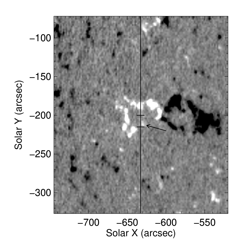
Figure 2.— A portion of an MDI magnetogram taken on 2007 August 22 at 14:27 UT showing the area covered by the EIS spectroheliograms and the approximate location of the EIS slit during the sit-and-stare observation. The horizontal lines along the slit mark the location of the oscillation data analyzed in this paper, and the area of weak magnetic flux that is the focus of this analysis is marked with an arrow. The image has been scaled so that the range of magnetic fluxes displayed is $\pm 100$ Gauss.

Figure 3.— TRACE 171 Å (Fe IX/X) image taken on 2007 August 22 at 20:01:19 UT. The box shows the location of the EIS spectroheliograms taken before and after the sit-and-stare observations, and the vertical line with the box shows the location of the sit-and stare observation. The horizontal lines along the slit mark the location of the oscillation data analyzed in this paper.

Both magnetogram data from the SOHO Michelson Doppler Imager (MDI) and Hinode Solar Optical Telescope (SOT) and coronal images taken in the 171 Å (Fe IX/X) filter with the Transition Region and Coronal Explorer (TRACE) were also examined. The magnetograms, one of which is shown in Figure 2 with the location of the EIS slit for the sit-and-stare observation indicated, show an extended bipolar plage region without any visible sunspots. As can be seen in the magnetogram, the EIS slit crosses two regions of positive (white) polarity. The weaker one, which has a size of about 6″and is marked with an arrow, is the focus of this analysis.

Figure 4.— Coalignment of EIS and SOT. Top left: EIS spectroheliogram taken in O VI 184.12 Å at the same time as the spectroheliograms shown in Figure 1, the dark vertical line near the center marks the slit location for the sit-and-stare observations. Top right: MDI full disk magnetogram taken at 14:27 UT. Bottom right: Hinode SP magnetogram, taken between 18:03 UT and 19:01 UT, at the same time the Ca II H time sequence was taken. Bottom left: temporal average of the time sequence in Ca II H taken between 19:50 and 21:40 UT. The black circles in the bottom images encompass a small network bright point that overlaps with the EIS slit.

The TRACE images, one of which is shown in Figure 3, show that the western part of the region near the right edge of the box that outlines the edges of the second EIS spectroheliogram exhibits fan-like coronal structures extending radially out in all directions, while the eastern part consists of shorter loop structures that connect the opposite polarities. The full set of TRACE images that cover most of the time period covered by the context and sit-and-stare observations are included as a movie. The movie shows generally quiescent behavior in the fan-like structures, but multiple brightenings in the eastern loop system. The largest of these took place at around 01:31 UT on August 23 and shows a filament eruption, which resulted in a system of post-flare loops that are visible in the Fe XV 284.16 Å and Fe XVI 262.98 Å spectroheliograms in the right panels of Figure 1. Some of the loops in the eastern part cross the EIS slit location for the sit-and-stare observations, but they are for the most part north of the area we focus on.

We have also examined images taken with the Extreme Ultraviolet Imaging Telescope (EUVI, Wuelser et al., 2004) on the Ahead (A) and Behind (B) spacecraft of the Solar Terrestrial Relations Observatory (STEREO). EUVI observes the entire solar disk and the corona up to 1.4 R_☉ with a pixel size of 1.59″. On 2007 August 22, the separation angle of STEREO with Earth was 14.985$\arcdeg$ for spacecraft A and 11.442$\arcdeg$ for spacecraft B. Our target region was rather near the limb as seen from spacecraft A. EUVI/B, however, provided continuous on-disk images between 2007 August 22, 11:00 UT and 2007 August 23, 11:30 UT, which allowed us to study the development of the coronal structures of the region during the time of the EIS observations.

We produced movies in all four EUVI channels (171 Å, 195 Å, 284 Å, and 304 Å), with 171 Å having the highest cadence of 2.5 min. The EUVI movies generally show the same behavior as that shown in the TRACE data. EUVI captured two larger events during this period, the first one started at around 12:24 UT on August 22, showing multiple brightenings of the eastern loop system although it is not clear if a CME had been launched. The second one took place at around 01:31 UT on August 23, involving the western part of the region and shows a filament eruption with a system of post-flare loops evolving at the time the second EIS context spectroheliogram was taken.

SOT obtained Ca II H observations at a one-minute cadence during the time interval of the sit-and-stare observations that are the focus of this study. To coalign those observations we use an EIS O VI 184.12 Å spectroheliogram, MDI magnetograms, SOT Spectro-Polarimeter (SP) magnetograms, and SOT Ca II H line filtergrams. The EIS O VI 184.12 Å spectroheliogram was part of the scan shown in Figure 1 (left), taken several hours before the sit-and-stare observations. Coalignment was carried out by rescaling the images, using cross-correlation techniques to overlap the selected subfields and finally blinking the images to ensure minimal offsets.

Figure 4 displays the O VI 184.12 Å spectroheliogram in the top left corner, with the dark vertical line representing the slit position of the sit-and-stare observations. The top right image is from a full-disk MDI magnetogram taken at 14:27 UT. The three small structures in the lower left corner of the magnetogram were used to coalign the O VI image, which shows bright emission structures at the same locations. In the next step we use SP data to coalign with the MDI magnetogram. The SP was scanning the target region on 2007 August 22 between 18:03 UT and 19:01 UT, at the same time the Ca II H image sequence was taken. The lower right image in Figure 4 gives the apparent longitudinal field strength as derived from the Stokes spectra. Comparing the two magnetograms we can see that the overall structure of the bi-polar region has hardly evolved over time and that the SP data show considerable additional fine structure in the magnetic field. We also note that in the time between the MDI magnetogram and SP magnetogram flux cancellation has taken place at the polarity inversion line of the bi-polar region (at around $x=-610$″). The eruption observed a few hours later in EUVI and TRACE was probably triggered by this flux cancellation.

Figure 5.— EIS sit-and-stare Doppler-shift data in four emission lines covering the entire sit-and-stare observation. The Doppler shift in each window has been adjusted so that the zero value is the average over the window. The maximum and minimum values plotted in each case are $+20$ and $-20$ km s^-1, respectively. This study focuses on the spatial range from $-200$″ to $-215$″ in the time interval from 20:07 to 21:53 UT.

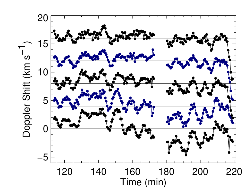
Figure 6.— Doppler shift data averaged over the 16 detector rows from $-200$″ to $-215$″. The emission lines shown from top to bottom are Fe XI 188.23 Å, Fe XII 195.12 Å, Fe XIII 202.04 Å, Fe XIV 274.20 Å, and Fe XV 284.16 Å. Time is measured in minutes from the start of the sit-and-stare data at 18:13:06 UT. The zero value for Doppler shifts is set to the average Doppler shift in each line and is shown using the horizontal lines. Data for each emission line are displaced from the next set by 4 km s^-1.

The target area for the oscillation study is in the black circle, a small magnetic region of positive polarity. In the final coalignment step the SOT Ca II H images were coaligned with the SP scan. The bottom left image in Figure 4 shows the temporal average of the time sequence taken between 19:50 UT and 21:40 UT. The black circle encompasses a small network bright point that overlaps with the EIS slit and the region averaged along the slit in the analysis that is the focus of this paper. As we have already noted, the EIS spectroheliograms taken before and after the sit-and-stare observation show that considerable structural evolution has taken place. In the Fe XV 264.78 Å spectroheliogram taken after the sit-and-stare observation, there is significant emission within the 6″ region of the EIS slit that is the focus of this paper, suggesting that the location is near one end of one of the coronal loops seen in the lower three panels in the right side of Figure 1. On the other hand the images in the EIS spectroheliograms taken immediately before the sit-and-stare observation show much less evidence for a loop rooted at that location. Thus we can only conclude that the bright feature we observe in the Ca II H line may be the footpoint of a coronal loop. We do note, however, that there are no other strong magnetic concentrations close to the location of the region that is the focus of this study. The ones to the south-east are about 10″ away—more than our co-alignment errors. We believe that loop footpoints will be anchored in strong flux concentrations.

The basic building block for the sit-and-stare observation was EIS Study ID 56. This study takes 50 30 s exposures in 20 spectral windows with a solar $y$-position coverage of 400″. The entire sit-and-stare observation consisted of four executions of the study, with each execution invoked with a repetition count of four. Thus, the full sit-and-stare data set consists of 16 repetitions of the basic building block. There was a brief delay between each invocation of the study, leading to gaps in the resulting time series.

Over both orbital periods and shorter time intervals, the Hinode pointing fluctuates in both the solar $x$- and $y$-directions by up to about 3″ peak-to-peak. This is due to both spacecraft pointing variations and changes in the location of EIS relative to the location of the Sun sensors on the spacecraft. Studies of the latter variations have shown that they are well-correlated with similar variations observed in data from the Hinode X-Ray Telescope (XRT). We have therefore used a modified version of the software provided by the XRT team to compute the average $y$-position of each pixel along the slit over each exposure and then interpolated the fitted centroid positions onto a uniform $y$-position grid.

It is not, of course, possible to correct the sit-and-stare observations for fluctuations in the $x$-position on the Sun. Plots of the $x$-position pointing fluctuations show that they tend to be smoother than the $y$-direction fluctuations, and that they are dominated by the orbital period. If periodic Doppler shifts are present only in very small structures, we would thus expect the signal to show a modulation with the orbital period. Larger structures, $\geq 3$″ in the $x$-direction, that display coherent Doppler shifts should not be affected by the spacecraft $x$-position pointing variations.

Over much of the EIS slit during the sit-and-stare observation there is no evidence for interesting dynamical behavior in the Doppler shift observations. The portion of the slit that covers the brighter core area of the region does, however, show evidence for periodic changes in the Doppler shifts. Figure 5 shows the measured Doppler-shift data in four emission lines over this $y$-position range as a function of time. The gaps between each invocation of the study appear as wider pixels near 20, 22, and 0 UT. Note that the data are also affected by passage of the spacecraft through the South Atlantic Anomaly (SAA). A small region of compromised data appears near 19:30 UT, and major SAA passages are evident near 21:00 and 22:45 UT.

The display shows clear evidence for periodic fluctuations in all the emission lines at $y$-positions of roughly $-170$″ to $-180$″during the first hour shown in the plots. Periodic fluctuations are also visible over $y$-locations centered near $-210$″. Note that there is some evidence of longer period fluctuations, for example in the Fe XV 284.16 Å emission line. These fluctuations are probably the result of the correction for orbital line centroid shifts not fully removing those variations. In the remainder of this paper, we focus on the area near $-210$″ that shows evidence for oscillatory phenomena.

3. ANALYSIS

3.1. Doppler Shift Oscillations

As we noted earlier, solar $y$-positions between $-200$″ and $-215$″ show considerable oscillatory behavior, particularly in the set of data taken beginning at 20:07:01 UT. Figure 6 shows the averaged Doppler shift data over the time period of this set of observations for, from top to bottom, Fe XI 188.23 Å, Fe XII 195.12 Å, Fe XIII 202.04 Å, Fe XIV 274.20 Å, and Fe XV 284.16 Å. The Doppler shifts have been averaged over the 16 detector rows from $-200$″ to $-215$″. Data from 172 to 180 minutes were taken during SAA passage and have been removed from the plot.

The Doppler shift data over this portion of the EIS slit show clear evidence for low-amplitude, roughly 2–4 km s^-1, oscillatory behavior with a period near 10 minutes. For some of the time period, particularly after 180 minutes, there appears to be a clear trend for the oscillations to display increasing amplitude as a function of increasing temperature of line formation.

Table 1Periods and Amplitudes Detected in Doppler Shift and Intensity Data

	Wavelength	Log $T$	$P_{D}$	$\delta v$	$P_{I}$	$\delta I/I$
Ion	(Å)	(K)	(minutes)	(km s-1)	(minutes)	(%)
Fe XI	188.23	6.07	10.0	1.2	11.8	1.1
Fe XII	195.12	6.11	10.1	1.1	11.4	0.9
Fe XIII	202.04	6.20	09.1	1.3	11.2	1.4
Fe XIV	274.20	6.28	09.1	1.3	11.4	2.0
Fe XV	284.16	6.32	09.0	1.4	07.6	2.4

Because there is a significant gap in the Doppler shift data, neither Fourier time series analysis nor wavelet analysis is appropriate. Instead, we examine the time series by calculating periodograms using the approach outlined in Horne & Baliunas (1986) and Press & Rybicki (1989). Figure 7 shows the periodograms calculated from the Doppler shift data shown in Figure 6. Also plotted on the figure are the 99% and 95% significance levels. All but one of the time series show a peak in the periodogram at the 99% confidence level, and the largest peak in the Fe XV 284.16 Å emission line data is at the 95% confidence level. Table 1 lists the period of the most significant peak in each of the panels shown in the figure.

To estimate the amplitude of the oscillations, we detrend the Doppler shift time series by subtracting a background computed using averaged data in a 10-minute window centered on each data point and then compute the rms amplitude as the standard deviation of the mean. For a sine wave, the peak velocity is the rms value multiplied by $\sqrt{2}$. These peak velocity values are also listed in the table in the $\delta v$ column. Visual inspection of the data suggests that the numbers in the table are smaller than what might be obtained by fitting the data. The numbers do confirm the impression that the oscillation amplitude increases with increasing temperature of line formation.

It is clear from the Doppler shift plots in Figure 6 that the oscillations are not always present. Instead, they appear for a few periods and then disappear. To understand better this behavior, we have fitted the time intervals where oscillations are obvious with a combination of a damped sine wave and a polynomial background. Thus, for each time period where oscillations are present we assume that the data can be fitted with a function of the form

$$v(t)=A_{0}\sin(\omega t+\phi)\exp(-\lambda t)+B(t),$$ (1)

where

$$B(t)=b_{0}+b_{1}t+b_{2}t^{2}+b_{3}t^{3}+\cdots$$ (2)

is the trend in the background data. Time is measured from an initial time $t_{0}$, which is different for each set of oscillations we fit. The fits were carried out using Levenberg-Marquardt least-squares minimization (Bevington, 1969). Generally only two terms in the background polynomial were necessary.

Figure 7.— Periodograms computed for the Doppler shift data shown in Figure 6. The solid horizontal line on each plot indicates the power equivalent to a calculated false alarm probability of 1% and the dashed line is for a false alarm probability of 5%.

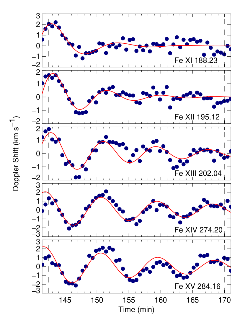
Figure 8.— Decaying sine wave fits to the Doppler shift data beginning roughly 142 minutes after the start of the sit-and-stare observation. The plotted data has had the polynomial background removed. Vertical dashed lines show the time range used in the fitting.

Figure 8 shows the results of this fitting for the Doppler shift data beginning 142.5 minutes after the start of the sit-and-stare observation. All the fits show roughly the same amplitudes, periods, and phases. Emission lines formed at the higher temperatures (Fe XIV and Fe XV) show clear evidence for more than one full oscillation period. At lower temperatures, the oscillatory signal damps much more rapidly.

Table 2 lists the amplitudes, $A_{0}$, periods, $P$, phases, $\phi$, and the inverse of the decay rate, $\lambda$, that result from fitting all the time periods in the data for which a reasonable fit to the Doppler shift data could be obtained. The periods are consistent with the results of the periodogram analysis for the entire time interval. Generally, the amplitudes are larger than the $\delta v$ values show in Table 1. Note that some of the fits show negative decay times, indicating that some of the oscillations show a tendency to grow with time. In these cases, this is not followed by a decay, but rather a rapid loss of the oscillatory signal.

All the fits use the start times $t_{0}$ listed in the table and thus the phase values for each time interval can not be directly compared. When the phases are adjusted to a common start time, the values do not agree. Thus while the periods are similar for each time interval in which oscillations are observed, it appears that each event is being independently excited.

Table 2Doppler Shift Oscillation Properties

$t_{0}$		$A_{0}$	$P$	$\phi$	$\lambda^{-1}$
(min)	Ion	(km s-1)	(min)	(rad)	(min)
113.9	Fe XI	0.9	08.8	1.8	+0019.0
113.9	Fe XII	0.7	09.2	2.3	$-216$
113.9	Fe XIII	0.7	08.8	2.3	00$-73.3$
113.9	Fe XIV	0.3	10.7	3.9	00$-10.9$
113.9	Fe XV	0.5	09.5	2.9	00$-24.5$
142.5	Fe XI	2.4	10.4	1.0	+005.1
142.5	Fe XII	2.0	08.4	0.9	+006.6
142.5	Fe XIII	1.6	08.2	1.2	+0015.0
142.5	Fe XIV	2.0	08.7	1.9	+0023.9
142.5	Fe XV	2.2	08.9	2.1	+0023.3
190.0	Fe XI	0.3	08.8	4.7	$-411$
190.0	Fe XII	0.8	07.5	3.5	+0036.8
190.0	Fe XIII	1.2	07.3	3.1	+0036.3
190.0	Fe XIV	1.5	07.3	3.2	+0043.6
190.0	Fe XV	2.2	07.5	3.4	+0012.8

Examining the amplitude of the oscillations in each time interval as a function of the temperature of line formation shows no clear trend. The data set starting at 113.9 minutes seems to show evidence for a decrease in amplitude with increasing temperature, while the data set beginning at 190.0 minutes shows the opposite trend. Similarly, there is no clear trend in the periods of the oscillations in each data set as a function of temperature.

3.2. Intensity Oscillations

If the observed Doppler shift oscillations are acoustic in nature, then they should also be visible in the intensity data. For a linear sound wave $v=c_{\textrm{s}}\delta\rho/\rho$, where $v$ is the amplitude of the wave, $c_{\textrm{s}}$ is the sound speed, and $\delta\rho$ is the density perturbation on the background density $\rho$. Taking an amplitude of 2 km s^-1, yields values of $\delta\rho/\rho$ of around 1%. Since the intensity fluctuation, $\delta I/I$, is proportional to $2\delta\rho/\rho$, we expect only about a 2% fluctuation in the measured intensity. This number could of course increase if the actual velocity is much larger due to a large difference between the line-of-sight and the direction of the coronal structure being measured. Figure 9 shows the measured intensity data averaged over the same locations as the Doppler shift data shown in Figure 6. The data show little or no evidence for oscillations with the periods measured in the Doppler shift data. This is borne out by a periodogram analysis of the time series in the figure, which show no significant peaks.

If, however, we detrend the data by subtracting the gradually evolving background signal, there is some evidence for an oscillatory signal. Figure 10 shows the data in Figure 9 with a background consisting of a 10-minute average of the data centered on each data point subtracted. All the emission lines show some evidence for an oscillatory signal, with the Fe XIII 202.04 Å emission line being the most obvious.

Figure 9.— Normalized intensity data averaged over the 16 detector rows from $-200$″ to $-215$″. The emission lines shown from top to bottom are Fe XI 188.23 Å, Fe XII 195.12 Å, Fe XIII 202.04 Å, Fe XIV 274.20 Å, and Fe XV 284.16 Å. Time is measured in minutes from the start of the sit-and-stare data at 18:13:06 UT. Data for each emission line are displaced from the next set by 0.2.

Figure 10.— Detrended intensity data averaged over the 16 detector rows from $-200$″ to $-215$″. The emission lines shown from top to bottom are Fe XI 188.23 Å, Fe XII 195.12 Å, Fe XIII 202.04 Å, Fe XIV 274.20 Å, and Fe XV 284.16 Å. Time is measured in minutes from the start of the sit-and-stare data at 18:13:06 UT. Data for each emission line are displaced from the next set by 100 ergs cm^-2 s^-1 sr^-1.

Figure 11.— Periodograms computed for the detrended intensity data shown in normalized form in Figure 9. The solid horizontal line on each plot indicates the power equivalent to a calculated false alarm probability of 1% and the dashed line is for a false alarm probability of 5%.

Figure 12.— Decaying sine wave fits to the detrended intensity data beginning roughly 138 minutes after the start of the sit-and-stare observation. The intensities have been converted to residual intensities by taking the difference between the intensity at each data point and the running mean intensity and dividing it by the running mean. The plotted data has also had the polynomial background used in the fit removed. Vertical dashed lines show the time range used in the fitting. Also plotted as green curves on the panels for the Fe XIV and Fe XV intensity data are the fitting results for the Fe XIV and Fe XV Doppler shift data. Those plots show $-v(t)$.

Figure 11 shows periodograms constructed for the emission lines shown in Figure 10. Each periodogram shows a significant peak. The periods for the strongest peak in each periodogram are listed in Table 1. The periods are generally consistent with those determined from the Doppler shift data. Also listed in the table is an estimate of the intensity fluctuation in each emission line. This was obtained by computing the standard deviation of the detrended intensity in the time series for each emission line and then dividing the result by the average intensity. The values are roughly consistent with those expected based on the $\delta v$ estimates listed in Table 1.

While the oscillatory signal is much less strong in the detrended intensity data than in the Doppler shift data, it is possible to fit some of the data in roughly the same time intervals that were used for the results listed in Table 2. Table 3 shows the resulting fit information. Note that intensity oscillation fits were not possible for all the lines for which the Doppler shift data could be fitted. Figure 12 shows an example of the fits to the detrended intensity data. For these plots the intensity has been converted to a residual intensity expressed in % by taking the difference between each data point and the 10-minute average and dividing it by the 10-minute average. The plotted points have also had the polynomial background subtracted.To facilitate comparisons with the Doppler shift data we have also plotted as green curves on the panels for the Fe XIV and Fe XV intensity data the fitting results for the Fe XIV and Fe XV Doppler shift data.

Comparison of the fits in Figure 12 with those in Figure 8 shows some similarities and many differences between the two data sets. For the lines with a reasonably strong signal, the periods measured for the residual intensity data are similar to those measured for the Doppler shifts. In addition, the residual intensities show the same trend to larger amplitudes as the temperature of line formation increases. The intensity oscillations clearly start earlier than the Doppler shift oscillations. Moreover, while the Doppler shift oscillations are damped, the intensity oscillations appear to grow with time over the same interval. This appears to be the case for the other time intervals as well. Fitting the detrended intensity signal is more challenging than fitting the Doppler shift signal. Also, implicit in the fitting is the idea that a damped sine wave can fully represent what is probably a more complex signal. Thus, we are reluctant to read too much into this growth in the intensity until we can determine from additional data sets if it is a common phenomenon.

Table 3Intensity Oscillation Properties

$t_{0}$		$A_{0}$	$P$	$\phi$	$\lambda^{-1}$
(min)	Ion	(%)	(min)	(rad)	(min)
113.9	Fe XII	2.1	08.0	4.2	+08.2
113.9	Fe XIII	1.0	12.3	4.4	+37.6
137.7	Fe XI	0.2	12.7	0.0	$-11.4$
137.7	Fe XII	0.4	10.3	3.9	$-17.8$
137.7	Fe XIII	1.1	09.9	3.5	$-50.2$
137.7	Fe XIV	2.1	09.3	3.0	$-41.8$
137.7	Fe XV	2.6	09.3	3.0	$-48.6$
190.0	Fe XI	0.5	08.8	5.0	$-81.1$
190.0	Fe XII	0.4	13.7	3.7	$-32.6$
190.0	Fe XIII	1.1	13.5	3.8	$-83.6$
190.0	Fe XIV	0.8	12.8	2.5	$-20.3$
190.0	Fe XV	1.3	06.9	5.6	$-22.8$

An important factor in determining the nature of the oscillations is the phase difference between the Doppler shift signal and the intensity signal. Comparing the phases of the fits listed in Table 2 with those in Table 3 is difficult because the periods are not identical, but, since the periods are close, the differences do not significantly alter any conclusions that we might draw. To facilitate this comparison we have plotted as green curves on the panels for the Fe XIV and Fe XV intensity data in Figure 12 the fitting results for the Fe XIV and Fe XV Doppler shift data. For the Doppler shift data, we plot $-v(t)$. The curves show that for these two ions, the intensity variations are close to $180\arcdeg$ out of phase with the Doppler shift variations. Since we define the Doppler shift as $c\,\delta\lambda/\!\lambda$, this means that the peak intensity corresponds to a blueshift, indicating an upward propagating wave. For the other two time intervals, the situation is more ambiguous. Examination of the tables shows that in many cases, the periods are significantly different for the same Doppler shift and intensity data in the same line. In those cases where the periods are close (e.g., Fe XII at $t_{0}=113.9$ minutes and Fe XV at $t_{0}=190.0$ minutes), examination of the plots similar to Figures 8 and 12 shows the same $180\arcdeg$ phase shift, again indicating upwardly propagating oscillations.

Even for the cases where the periods are close, the agreements in the phases are only approximate. For the Fe XIV and Fe XV intensity and Doppler shift fits shown in Figure 12, the intensity oscillation leads the Doppler shift oscillation by a small fraction of a period. For both the Fe XII data at $t_{0}=113.9$ minutes and the Fe XV data at $t_{0}=190.0$ minutes, the Doppler shift oscillation leads the intensity oscillation by a fraction of a period. In both cases, this difference is less than the $1/4$ period expected for a standing-mode MHD wave (Sakurai et al., 2002). Wang et al. (2009a) observed propagating waves with periods in the four to six minute range in EIS active region observations. They noted that for most cases the Doppler shift and intensity oscillations were nearly in phase. In the cases where there was a difference, the phase of the intensity was earlier than the Doppler shift, as is the case for the data shown in Figures 8 and 12. Theoretical modeling of propagating slow waves with periods near five minutes show that thermal conduction can produce phase shifts between the intensity and Doppler shifts (Owen et al., 2009). Further study of EIS data sets where both the Doppler shift and intensity can be fitted could provide valuable constraints on these models.

3.3. Density Oscillations

The electron density is one factor in determining the Alfvén speed in the oscillating plasma. Moreover, for magnetoacoustic fluctuations, we expect the density to also oscillate. Thus a direct measurement can aid in disentangling the nature of the oscillations. The sit-and-stare observations included density-sensitive line pairs of Fe XII (186.88 Å/195.12 Å) and Fe XIII (203.83 Å/202.04 Å). Using data from version 5.2 of the CHIANTI database (Landi et al., 2006; Dere et al., 1997), we computed the electron density at each time for the row-averaged data. For Fe XII, CHIANTI uses energy levels and radiative decay rates from Del Zanna & Mason (2005), electron collision strengths from Storey et al. (2005), and proton collision rate coefficients from Landman (1978). For Fe XIII, CHIANTI uses energy levels from Penn & Kuhn (1994), Jupen et al. (1993), and version 1.0 of the NIST database; radiative decay rates from Young (2004), electron collision strengths from Gupta & Tayal (1998), and proton collision rate coefficients from Landman (1975). These diagnostics are discussed in detail in Young et al. (2009).

Figure 13.— Electron density determined using the Fe XII 186.88 Å/195.12 Å ratio (top) and the Fe XIII 203.83 Å/202.04 Å ratio (bottom) for the data beginning roughly 138 minutes after the start of the sit-and-stare observation.

Figure 13 shows the derived electron densities as a function of time for the same time interval shown in Figures 8 and 12. Both sets of derived densities show the same overall time behavior, but the absolute values differ by nearly a factor of three. Differences between these diagnostics have been noted before (e.g., Young et al., 2009), and are thought to be due to issues with the atomic data. It is not yet clear which of the values should be considered the most reliable.

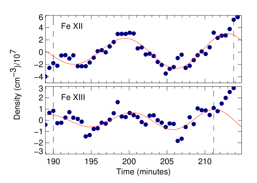
Figure 14.— Decaying sine wave fits to the smoothed electron density determined using the Fe XII 186.88 Å/195.12 Å ratio (top) and the Fe XIII 203.83 Å/202.04 Å ratio (bottom) for the data beginning 190 minutes after the start of the sit-and-stare observation along with. The plotted data has had the polynomial background removed. Vertical dashed lines show the time range used in the fitting.

Neither of the density time series shown in the figure display any evidence for the oscillations detected in the detrended intensity data. If we smooth the density time series with a 10-minute running mean, there is some evidence for oscillatory behavior over the time range beginning at 190 minutes. Decaying sine wave fits to that region are show in Figure 14. For the Fe XII time series the fit has an amplitude of $1.9\times 10^{7}$ cm^-3, a period of 13.5 minutes, a decay time of $-46.4$ minutes, and a phase of 3.5 radians, all consistent with the values listed for the Fe XII data in Table 3 for this time interval. For the Fe XIII time series the fit has an amplitude of $5.1\times 10^{6}$ cm^-3, a period of 10.9 minutes, a decay time of $-25.1$ minutes, and a phase of 1.9 radians. With the exception of the phase, these values are generally consistent with the Fe XIII data in Table 3 for this time interval. The amplitudes for the Fe XII and Fe XIII fits are 0.5% and 0.4% of the average density in the time interval. Since the observed intensity fluctuations are only about 1%, though, and we expect $\delta I/I$ to be proportional to $2\delta\rho/\rho$, they are consistent with the observed intensity oscillations.

3.4. Underlying Chromospheric Behavior

As we pointed out earlier, SOT obtained a time sequence of Ca II H images that is co-temporal with the EIS sit-and-stare observations starting at 19:50 UT and ending at 21:40 UT, with a constant cadence of 60 s. To further use this data, we applied the standard reduction procedure provided by the SOT team that is available in SolarSoft. The images of the Ca II H sequence were then carefully aligned using Fourier cross-correlation techniques to remove residual jitter and the drift of the SOT correlation tracker.

As can be seen in the lower left panel of Figure 4, the EIS slit covers the network bright point, which is the focus of the chromospheric analysis. Considering the accuracy of the coalignment and the spatial averaging applied to the EIS data, we also average the Ca II H signal.

Figure 15 shows the time history of the Ca II H-line intensity for three different sized spatial areas centered on the feature shown in Figure 4. The sizes of the regions are given in SOT pixels, which are $0.10896$″ in size. As expected for chromospheric lines, all three averaged data sets show evidence for intensity oscillations with a period near 5 minutes. The data, however, are quite noisy and periodograms constructed from them show no significant peaks. Detrending the data, however, results in periodograms with significant peaks. Figure 16 shows periodograms for the three data sets with each detrended by subtracting a 9-minute running mean from each data point. The periodograms show clear evidence for oscillations near 5 minutes.

Figure 15.— Ca II H intensity data averaged over different spatial areas centered on the magnetic feature highlighted in Figure 4. Each data set has had the mean value subtracted. Spatial areas are given in SOT pixels, which are 0.10896″in size, giving areas of $2.18\arcsec\times 2.18\arcsec$, $3.77\arcsec\times 3.77\arcsec$, and $4.36\arcsec\times 4.36\arcsec$, respectively.

Figure 16.— Periodograms computed for the detrended Ca II H intensity data. The size of the area averaged over in pixels in indicated in each plot. The solid horizontal line on each plot indicates the power equivalent to a calculated false alarm probability of 1% and the dashed line is for a false alarm probability of 5%. Spatial areas are given in SOT pixels, which are 0.10896″in size, giving areas of $2.18\arcsec\times 2.18\arcsec$, $3.77\arcsec\times 3.77\arcsec$, and $4.36\arcsec\times 4.36\arcsec$, respectively.

There is also some evidence for power at periods between 9 and 10 minutes, but with more than a 5% false alarm probability. If we instead detrend the data with an 11-minute running mean, then the peak between 9 and 10 minutes becomes more prominent and is at or above the 5% false alarm probability level for the $30~{}\mathrm{pixel}\times 30~{}\mathrm{pixel}$ and $20~{}\mathrm{pixel}\times 20~{}\mathrm{pixel}$ data sets. Wavelet analysis of the data sets detrended with both a 9- and 11-minute running mean shows significant signal near 9 minutes.

Note that the data in Figure 15 shows three larger peaks in all three data sets. The first peak, near 110 minutes, occurs before the beginning of the EIS data plots in Figures 6 and 10. The other two, at roughly 140 and 170 minutes, come just before significant oscillatory signal is observed in the EIS Doppler shift and detrended intensity data. It is tempting to suggest that these enhancements correspond to chromospheric events that resulted in the oscillations observed with EIS.

In principle the EIS He II 256.32 Å data can bridge the gap in temperature between the SOT Ca II data and the Fe lines formed at higher temperatures that are the main focus of this study. In practice the He II data are challenging to analyze. The line is closely blended with a Si X line at 256.37 Å along with a smaller contribution from Fe X and Fe XIII ions at slightly longer wavelengths (Brown et al., 2008). In an effort to see if a connection can be made, we have made two-component Gaussian fits to the row-averaged He II data. Periodograms of the resulting Doppler shift data show no significant periods. Periodograms of the He II fitted intensities detrended with a 10-minute running mean show no peaks at the 1% false alarm probably level and one peak with a period between 12 and 13 minutes at the 5% false alarm probability level. Examining the detrended He II intensity data, we do not see a peak in the data at 140 minutes, but do see a significant increase at 170 minutes. Thus the He II data only weakly support our suggestion that the enhancements seen in the Ca II data correspond to chromospheric events that result in the oscillations observed with EIS in the Fe lines.

4. DISCUSSION AND CONCLUSIONS

As we pointed out in §1, a number of investigations have detected Doppler shift oscillations with EIS. Based on the phase differences between the Doppler shift and the intensity, we believe that the signals we have detected are upwardly propagating magnetoacoustic waves. The periods we detect are between 7 and 14 minutes. For a set of observations that begins at a particular time, there is considerable scatter in the measured periods and amplitudes. This is probably due to the relatively weak signal we are analyzing. But it may also be an indication that a simple sine wave fit is not a good representation of the data. It is likely that each line-of-sight passes through a complex, time-dependent dynamical system. While a single flux tube may respond to an oscillatory signal by exhibiting a damped sine wave in the Doppler shift, a more complex line-of-sight may display a superposition of waves.

Coalignment of the EIS data with both SOT and MDI magnetograms shows that the portion of the EIS slit analyzed in this study corresponds to a unipolar flux concentration. SOT Ca II images show that the intensity of this feature exhibits 5-minute oscillations typical of chromospheric plasma, but also exhibits some evidence for longer period oscillations in the time range detected by EIS. Moreover, the Ca II intensity data show that the oscillations observed in EIS are related to significant enhancements in the Ca II intensities, suggesting that a small chromospheric heating event triggered the observed EIS response.

Wang et al. (2009a) also detected propagating slow magnetoacoustic waves in an active region observed with EIS, which they associated with the footpoint of a coronal loop. While the oscillation periods they measured—5 minutes—were smaller than those detected here, many of the overall characteristics we see are the same. In each case, the oscillation only persists for a few cycles and the phase relationship indicates an upwardly propagating wave. In contrast with their results, however, we do not see a consistent trend for the oscillation amplitude to decrease with increasing temperature of line formation. Examination of both the Doppler shift data in Figure 6 and the results in Table 2 shows that in one case the amplitude has a tendency to decrease with increasing temperature of line formation (oscillation beginning at 113.9 minutes) and in another case the amplitude clearly increases with increasing temperature of line formation (oscillation beginning at 190 minutes). Thus it does not appear that the results reported by Wang et al. (2009a) are always the case. O’Shea et al. (2002) noted that for oscillations observed above a sunspot the amplitude decreased with increasing temperature until the temperature of formation of Mg X, which is formed at roughly 1 MK. They then saw an increase in amplitude in emission from Fe XVI. All the EIS lines we have included in this study have temperatures of formation greater than 1 MK.

Combined EIS and SUMER polar coronal hole observations have also shown evidence propagating slow magnetoacoustic waves (Banerjee et al., 2009). These waves have periods in the 10–30 minute range. These waves appear to be more like those we observe in that they are have periods longer than those studied by Wang et al. (2009a).

Wang et al. (2009a) suggested that the waves they observed were the result of leakage of photospheric p-mode oscillations upward into the corona. The longer periods we and Banerjee et al. (2009) observe are probably not related to p-modes. Instead, we speculate that the periods of the waves are related to the impulsive heating which may be producing them. If an instability is near the point where rather than generating a catastrophic release of energy it wanders back and forth between generating heating and turning back off, waves would be created. The heating source could be at a single location, or, for example, locations near each other where instability in one place causes a second nearby location to go unstable and begin heating plasma. In this view, the periods provide some insight into the timescale for the heating to rise and fall and thus may be able to place limits on possible heating mechanisms.

The behavior of slow magnetoacoustic oscillations as a function of temperature has been the subject of considerable theoretical work. It is generally believed that the damping of the waves is due to thermal conduction (e.g., De Moortel & Hood, 2003; Klimchuk et al., 2004). Because thermal conduction scales as a high power of the temperature, conductive damping should be stronger for oscillations detected in higher temperature emission lines (e.g., Porter et al., 1994; Ofman & Wang, 2002). Earlier EIS observations of the damping of standing slow magnetoacoustic waves, however, show that this is not always the case (Mariska et al., 2008). Thus, the temperature behavior of both the amplitude of the oscillations and the damping, differ from some earlier results. We believe that additional observations will be required to understand fully the physical picture of what is occurring in the low corona when oscillations are observed. Given the complex set of structures that may be in the line of sight to any given solar location under the EIS slit, we are not entirely surprised that different data sets should yield different results, which in some cases differ from models. For example, none of the current models for oscillations in the outer layers of the solar atmosphere take into account the possibility that what appear to be single structures in the data might actually be bundles of threads with differing physical conditions.

Our observations along with others (e.g., Wang et al., 2009a, b; Banerjee et al., 2009) show that low-amplitude upwardly propagating slow magnetoacoustic waves are not uncommon in the low corona. The periods observed to date range from 5 minutes to 30 minutes. In all cases, however, the wave amplitudes are too small to contribute significantly to coronal heating. But understanding how the waves are generated and behave as a function of line formation temperature and the structure of the magnetic field should lead to a more complete understanding of the structure of the low corona and its connection with the underlying portions of the atmosphere. Instruments like those on Hinode that can simultaneously observe both the chromosphere and the corona, should provide valuable additional insight into these waves as the new solar cycle rises and more active regions become available for study.

References

- Aschwanden et al. (1999) Aschwanden, M. J., Fletcher, L., Schrijver, C. J., & Alexander, D. 1999, ApJ, 520, 880
- Banerjee et al. (2009) Banerjee, D., Teriaca, L., Gupta, G. R., Imada, S., Stenborg, G., & Solanki, S. K. 2009, A&A, 499, L29
- Berghmans & Clette (1999) Berghmans, D., & Clette, F. 1999, Sol. Phys., 186, 207
- Bevington (1969) Bevington, P. R. 1969, Data reduction and error analysis for the physical sciences (New York: McGraw-Hill)
- Brown et al. (2008) Brown, C. M., Feldman, U., Seely, J. F., Korendyke, C. M., & Hara, H. 2008, ApJS, 176, 511
- Culhane et al. (2007) Culhane, J. L., et al. 2007, Sol. Phys., 243, 19
- De Moortel & Hood (2003) De Moortel, I., & Hood, A. W. 2003, A&A, 408, 755
- DeForest & Gurman (1998) DeForest, C. E., & Gurman, J. B. 1998, ApJ, 501, L217
- Del Zanna & Mason (2005) Del Zanna, G., & Mason, H. E. 2005, A&A, 433, 731
- Dere et al. (1997) Dere, K. P., Landi, E., Mason, H. E., Monsignori Fossi, B. C., & Young, P. R. 1997, A&AS, 125, 149
- Gupta & Tayal (1998) Gupta, G. P., & Tayal, S. S. 1998, ApJ, 506, 464
- Horne & Baliunas (1986) Horne, J. H., & Baliunas, S. L. 1986, ApJ, 302, 757
- Jupen et al. (1993) Jupen, C., Isler, R. C., & Trabert, E. 1993, MNRAS, 264, 627
- Klimchuk et al. (2004) Klimchuk, J. A., Tanner, S. E. M., & De Moortel, I. 2004, ApJ, 616, 1232
- Kosugi et al. (2007) Kosugi, T., et al. 2007, Sol. Phys., 243, 3
- Landi et al. (2006) Landi, E., Del Zanna, G., Young, P. R., Dere, K. P., Mason, H. E., & Landini, M. 2006, ApJS, 162, 261
- Landman (1975) Landman, D. A. 1975, A&A, 43, 285
- Landman (1978) —. 1978, ApJ, 220, 366
- Mariska et al. (2008) Mariska, J. T., Warren, H. P., Williams, D. R., & Watanabe, T. 2008, ApJ, 681, L41
- Ofman & Wang (2002) Ofman, L., & Wang, T. 2002, ApJ, 580, L85
- O’Shea et al. (2002) O’Shea, E., Muglach, K., & Fleck, B. 2002, A&A, 387, 642
- Owen et al. (2009) Owen, N. R., De Moortel, I., & Hood, A. W. 2009, A&A, 494, 339
- Penn & Kuhn (1994) Penn, M. J., & Kuhn, J. R. 1994, ApJ, 434, 807
- Porter et al. (1994) Porter, L. J., Klimchuk, J. A., & Sturrock, P. A. 1994, ApJ, 435, 482
- Press & Rybicki (1989) Press, W. H., & Rybicki, G. B. 1989, ApJ, 338, 277
- Roberts (2000) Roberts, B. 2000, Sol. Phys., 193, 139
- Roberts et al. (1983) Roberts, B., Edwin, P. M., & Benz, A. O. 1983, Nature, 305, 688
- Roberts et al. (1984) —. 1984, ApJ, 279, 857
- Roberts & Nakariakov (2003) Roberts, B., & Nakariakov, V. M. 2003, in NATO Science Series: II: Mathematics, Physics and Chemistry, Vol. 124, Turbulence, Waves and Instabilities in the Solar Plasma, ed. R. Erdelyi, K. Petrovay, B. Roberts, & M. J. Aschwanden (Kluwer Academic Publishers, Dordrecht), 167–192
- Rosenberg (1970) Rosenberg, H. 1970, A&A, 9, 159
- Sakurai et al. (2002) Sakurai, T., Ichimoto, K., Raju, K. P., & Singh, J. 2002, Sol. Phys., 209, 265
- Storey et al. (2005) Storey, P. J., Del Zanna, G., Mason, H. E., & Zeippen, C. J. 2005, A&A, 433, 717
- Van Doorsselaere et al. (2008) Van Doorsselaere, T., Nakariakov, V. M., Young, P. R., & Verwichte, E. 2008, A&A, 487, L17
- Wang et al. (2002) Wang, T., Solanki, S. K., Curdt, W., Innes, D. E., & Dammasch, I. E. 2002, ApJ, 574, L101
- Wang et al. (2009a) Wang, T. J., Ofman, L., & Davila, J. M. 2009a, ApJ, 696, 1448
- Wang et al. (2009b) Wang, T. J., Ofman, L., Davila, J. M., & Mariska, J. T. 2009b, A&A, 503, L25
- Wuelser et al. (2004) Wuelser, J.-P., et al. 2004, in Society of Photo-Optical Instrumentation Engineers (SPIE) Conference Series, ed. S. Fineschi & M. A. Gummin, Vol. 5171, 111
- Young (2004) Young, P. R. 2004, A&A, 417, 785
- Young et al. (2009) Young, P. R., Watanabe, T., Hara, H., & Mariska, J. T. 2009, A&A, 495, 587