Abstract

We consider perfect simulation algorithms for locally stable point processes based on dominated coupling from the past, and apply these methods in two different contexts. A new version of the algorithm is developed which is feasible for processes which are neither purely attractive nor purely repulsive. Such processes include multiscale area-interaction processes, which are capable of modelling point patterns whose clustering structure varies across scales. The other topic considered is nonparametric regression using wavelets, where we use a suitable area-interaction process on the discrete space of indices of wavelet coefficients to model the notion that if one wavelet coefficient is non-zero then it is more likely that neighbouring coefficients will be also. A method based on perfect simulation within this model shows promising results compared to the standard methods which threshold coefficients independently.

Chapter 0 Perfect simulation using dominated coupling from the past with application to area-interaction point processes and wavelet thresholding

Graeme K. Ambler Bernard W. Silverman

Keywords

coupling from the past (CFTP), dominated CFTP, exact simulation, local stability, Markov chain Monte Carlo, perfect simulation, Papangelou conditional intensity, spatial birth-and-death process

AMS subject classification (MSC2010)

62M30, 60G55, 60K35

1 Introduction

Markov chain Monte Carlo (MCMC) is now one of the standard approaches of computational Bayesian inference. A standard issue when using MCMC is the need to ensure that the Markov chain we are using for simulation has reached equilibrium. For certain classes of problem, this problem was solved by the introduction of coupling from the past (CFTP) (Propp and Wilson,, 1996, 1998). More recently, methods based on CFTP have been developed for perfect simulation of spatial point process models (see for example Kendall, (1997, 1998); Häggström et al., (1999); Kendall and Møller, (2000)).

Exact CFTP methods are therefore attractive, as one does not need to check convergence rigorously or worry about burn-in, or use complicated methods to find appropriate standard errors for Monte Carlo estimates based on correlated samples. Independent and identically distributed samples are now available, so estimation reduces to the simplest case. Unfortunately, this simplicity comes at a price. These methods are notorious for taking a long time to return just one exact sample and are often difficult to code, leading many to give up and return to nonexact methods. In response to these issues, in the first part of this paper we present a dominated CFTP algorithm for the simulation of locally stable point processes which potentially requires far fewer evaluations per iteration than the existing method in the literature (Kendall and Møller,, 2000).

The paper then goes on to discuss applications of this CFTP algorithm, in two different contexts, the modelling of point patterns and nonparametric regression by wavelet thresholding. In particular it will be seen that these two problem areas are much more closely related than might be imagined, because of the way that the non-zero coefficients in a wavelet expansion may be modelled as an appropriate point process.

The structure of the paper is as follows. In Section 2 we discuss perfect simulation, beginning with ordinary coupling from the past (CFTP) and moving on to dominated CFTP for spatial point processes. We then introduce and justify our perfect simulation algorithm. In Section 3 we first review the standard area-interaction process. We then introduce our multiscale process, describe how to use our new perfect simulation algorithm to simulate from it, and discuss a method for inferring the parameter values from data, and present an application to the Redwood seedlings data. In Section 4 we turn attention to the wavelet regression problem. Bayesian approaches are reviewed, and a model introduced which incorporates an area-interaction process on the discrete space of indices of wavelet coefficients. In Section 5 the application of our perfect simulation algorithm in this context is developed. The need appropriately to modify the approach to increase its computational feasibility is addressed, and a simulation study investigating its performance on standard test examples is carried out. Sections 3 and 5 both conclude with some suggestions for future work.

2 Perfect simulation

1 Coupling from the past

In this section, we offer a brief intuitive introduction to the principle behind CFTP. For more formal descriptions and details, see, for example, Propp and Wilson, (1996), MacKay, (2003, Chapter 32) and Connor, (2007).

Suppose we wanted to sample from the stationary distribution of an irreducible aperiodic Markov chain $\{Z_{t}\}$ on some (finite) state space $X$ with states 1, …, $n$. Intuitively, if it were possible to go back an infinite amount in time and start the chain running, the chain would be in its stationary distribution when one returned to the present (i.e. $Z_{0}\sim\pi$, where $\pi$ is the stationary distribution of the chain).

Now, suppose we were to set not one, but $n$ chains $\{Z^{(1)}_{t}\}$, …, $\{Z^{(n)}_{t}\}$ running at a fixed time $-M$ in the past, where $Z^{(i)}_{-M}=i$ for each chain $\{Z^{(i)}_{t}\}$. Now let all the chains be coupled so that if $Z^{(i)}_{s}=Z^{(j)}_{s}$ at any time $s$ then $Z^{(i)}_{t}=Z^{(j)}_{t}$ $\forall t\geq s$. Then if all the chains ended up in the same state $j$ at time zero (i.e. $Z^{(i)}_{0}=j$ $\forall i\in X$), we would know that whichever state the chain passing from time minus infinity to zero was in at time $-M$, the chain would end up in state $j$ at time zero. Thus the state at time zero is a sample from the stationary distribution provided $M$ is large enough for coalescence to have been achieved for the realisations being considered.

When performing CFTP, a useful property of the coupling chosen is that it be stochastically monotone as in the following definition.

Definition 2.1.

Let $\{Z^{(i)}_{t}\}$ and $\{Z^{(j)}_{t}\}$ be two Markov chains obeying the same transition kernel. Then a coupling of these Markov chains is stochastically monotone with respect to a partial ordering $\preceq$ if whenever $Z^{(i)}_{t}\preceq Z^{(j)}_{t}$, then $Z^{(i)}_{t+k}\preceq Z^{(j)}_{t+k}$ for all positive $k$.

Whenever the coupling used is stochastically monotone and there are maximal and minimal elements with respect to $\preceq$ then we need only simulate chains which start in the top and bottom states, since chains starting in all other states are sandwiched by these two. This is an important ingredient of the dominated coupling from the past algorithm introduced in the next section.

Although attempts have been made to generalise CFTP to continuous state spaces (notably Murdoch and Green, (1998) and Green and Murdoch, (1998), as well as Kendall and Møller, (2000), discussed in Section 2), there is still much work to be done before exact sampling becomes universally, or even generally applicable. For example, there are no truly general methods for processes in high, or even moderate, dimensions.

2 Dominated coupling from the past

Dominated coupling from the past was introduced as an extension of coupling from the past which allowed the simulation of the area-interaction process (Kendall,, 1998), though it was soon extended to other types of point processes and more general spaces (Kendall and Møller,, 2000). We give the formulation for locally stable point processes.

Let $x$ be a spatial point pattern in some bounded subset $S\subset\mathbb{R}^{n}$, and $u$ a single point $u\in S$. Suppose that $x$ is a realisation of a spatial point process $X$ with density $f$ with respect to the unit rate Poisson process. The Papangelou conditional intensity $\lambda_{f}$ is defined by

$$\lambda_{f}(u;x)=\frac{f(x\cup\{u\})}{f(x)};$$

see, for example, Papangelou, (1974) and Baddeley et al., (2005). If the process $X$ is locally stable, then there exists a constant $\lambda$ such that $\lambda_{f}(u;x)\leq\lambda$ for all finite point configurations $x\subset S$ and all points $u\in S\setminus x$.

The algorithm given in Kendall and Møller, (2000) is then as follows.

1. Obtain a sample of the Poisson process with rate $\lambda$.

2. Evolve a Markov process $D(T)$ backwards until some fixed time $-T$, using a birth-and-death process with death rate equal to 1 and birth rate equal to $\lambda$. The configuration generated in step 1 is used as the initial state.

3. Mark all of the points in the process with U[0,1] marks. We refer to the mark of point $x$ as $P(x)$.

4. Recursively define upper and lower processes, $U$ and $L$ as follows. The initial configurations at time $-T$ for the processes are

   $$U_{-T}(-T) = \left\{x\;:x\in D(-T)\right\};$$

   $$L_{-T}(-T) = \left\{\boldsymbol{0}\right\}.$$

5. Evolve the processes forwards in time to $t=0$ in the following way.

   Suppose that the processes have been generated up a given time, $u$, and suppose that the next birth or death to occur after that time happens at time $t_{i}$. If a birth happens next then we accept the birth of the point $x$ in $U_{-T}$ or $L_{-T}$ if the point’s mark, $P(x)$, is less than

   $$\begin{split}&\min\left\{\frac{\lambda_{f}(x;X)}{\lambda}:L_{-T}(t_{i})\subseteq X\subseteq U_{-T}(t_{i})\right\}\ \text{or}\\ &\max\left\{\frac{\lambda_{f}(x;X)}{\lambda}:L_{-T}(t_{i})\subseteq X\subseteq U_{-T}(t_{i})\right\}\end{split}$$ (2.1)

   respectively, where $x$ is the point to be born.

   If, however, a death happens next then if the event is present in either of our processes we remove the dying event, setting $U_{-T}(t_{i})=U_{-T}(u)\setminus\{x\}$ and $L_{-T}(t_{i})=L_{-T}(u)\setminus\{x\}$.

6. Define $U_{-T}(u+\varepsilon)=U_{-T}(u)$ and $L_{-T}(u+\varepsilon)=L_{-T}(u)$ for $u<u+\varepsilon<t_{i}$.

7. If $U_{-T}$ and $L_{-T}$ are identical at time zero (i.e. if $U_{-T}(0)=L_{-T}(0)$), then we have the required sample from the area-interaction process with rate parameter $\lambda$ and attraction parameter $\gamma$. If not, go to step 2 and repeat, extending the underlying Poisson process back to $-(T+S)$ and generating additional $U[0,1]$ marks (keeping the ones already generated).

This algorithm involves calculation of $\lambda(u;X)$ for each configuration that is both a subset of $U(T)$ and a superset of $L(T)$. Since calculation of $\lambda(u;X)$ is typically expensive, this calculation may be very costly. The method proposed in Section 3 uses an alternative version of step 5 which requires us only to calculate $\lambda(u;X)$ for upper and lower processes.

The more general form given in Kendall and Møller, (2000) may be obtained from the above algorithm by replacing the evolving Poisson process $D(T)$ with a general dominating process on a partially ordered space $(\Omega,\preceq)$ with a unique minimal element $\boldsymbol{0}$. The partial ordering in the above algorithm is that induced by the subset relation $\subseteq$. Step 5 is replaced by any step which preserves the crucial funnelling property

$$L_{-T}(u)\preceq L_{-(T+S)}(u)\preceq U_{-(T+S)}(u)\preceq U_{-T}(u)$$ (2.2)

for all $u<0$ and $T$, $S>0$ and the sandwiching relations

$$L_{-T}(u)\preceq X_{-T}(u)\preceq U_{-T}(u)\preceq D(u)$$ and (2.3)

$$L_{-T}(t)=U_{-T}(t)\;\text{ if }\;L_{-T}(s)=U_{-T}(s)$$ (2.4)

for $s\leq t\leq 0$. In equation (2.3), $X_{-T}(u)$ is the Markov chain or process from whose stationary distribution we wish to sample.

3 A perfect simulation algorithm

Suppose that we wish to sample from a locally stable point process with density

$$p(X)=\alpha\prod_{i=1}^{m}f_{i}(X),$$ (2.5)

where $\alpha\in(0,\infty)$ and $f_{i}:\mathfrak{R}^{f}\to\mathbb{R}$ are positive-valued functions which are monotonic with respect to the partial ordering $\preceq$ induced by the subset relation and have uniformly bounded Papangelou conditional intensity:

$$\lambda_{f_{i}}(u;\mathbf{x})=\frac{f_{i}(\mathbf{x}\cup\{u\})}{f_{i}(\mathbf{x})}\leq K.$$ (2.6)

When the conditional intensity (2.6) can be expressed in this way, as the product of monotonic interactions, then we shall demonstrate that the crucial step of the Kendall–Møller algorithm may be re-written in a form which is computationally much more efficient, essentially by dealing with each factor separately.

Clearly

$$\lambda_{p}(u;\mathbf{x})\leq\lambda=\prod_{i=1}^{m}\max_{X,\{x\}}\lambda_{f_{i}}(x;X)$$ (2.7)

for all $u$ and $\mathbf{x}$, and $\lambda$ is finite. Thus we may use the algorithm in Section 2 to simulate from this process using a Poisson process with rate $\lambda$ as the dominating process.

However, as previously mentioned, calculation of $\lambda_{p}(u;\mathbf{x})$ is typically expensive, increasing at least linearly in $n(\mathbf{x})$. Thus to calculate the expressions in (2.1), we must in general perform $2^{n(U_{-T}(t_{i}))-n(L_{-T}(t_{i}))}$ of these calculations, making the algorithm non-polynomial. In practice it is clearly not feasible to use this algorithm in all but the most trivial of cases, so we must look for some way to reduce the computational burden in step 5 of the algorithm.

This can be done by replacing step 5 with the following alternative.

1. Evolve the processes forwards in time to $t=0$ in the following way.

   Suppose that the processes have been generated up a given time, $u$, and suppose that the next birth or death to occur after that time happens at time $t_{i}$. If a birth happens next then we accept the birth of the point $x$ in $U_{-T}$ or $L_{-T}$ if the point’s mark, $P(x)$, is less than

   $$\prod_{i=1}^{m}\left[\max\left\{\lambda_{f_{i}}(u;U(T)),\lambda_{f_{i}}(u;L(T))\right\}\left/\lambda\right.\right]$$ or (2.8)

   $$\prod_{i=1}^{m}\left[\min\left\{\lambda_{f_{i}}(u;U(T)),\lambda_{f_{i}}(u;L(T))\right\}\left/\lambda\right.\right]$$ (2.9)

   respectively, where $x$ is the point to be born.

   If, however, a death happens next then if the event is present in either of our processes we remove the dying event, setting $U_{-T}(t_{i})=U_{-T}(u)\setminus\{x\}$ and $L_{-T}(t_{i})=L_{-T}(u)\setminus\{x\}$.

Lemma 2.2.

Step $\ref{evolve}^{\prime}$ obeys properties $(\ref{funnel})$, $(\ref{sand1})$ and $(\ref{sand2})$, and is thus a valid dominated coupling-from-the-past algorithm.

Proof.

Property (2.3) follows by noting that

$$(\ref{gen-low})\leq\lambda_{p}(u;X)\leq(\ref{gen-up})\leq 1.$$

Property (2.4) is trivial. Property (2.2) follows from the monotonicity of the $f_{i}$. ∎

Theorem 2.3.

Suppose that we wish to simulate from a locally stable point process whose density $p(X)$ with respect to the unit-rate Poisson process is representable in form $(\ref{gen-proc})$. Then by replacing Step 5 by Step $\ref{evolve}^{\prime}$ it is possible to bound the necessary number of calculations of $\lambda_{p}(u;X)$ per iteration in the dominated coupling-from-the-past algorithm independently of $n(X)$.

Proof.

Step 5$\mbox{}^{\prime}$ clearly involves only a constant number of calculations, so by Lemma 2.2 above and Theorem 2.1 of Kendall and Møller, (2000), the result holds. ∎

In the case where it is possible to write $p(X)$ in form (2.5) with $m=1$, Step 5$\mbox{}^{\prime}$ is identical to Step 5. This is the case for models which are either purely attractive or purely repulsive, such as the standard area-interaction process discussed in Section 1. It is not the case for the multiscale process discussed in Section 2, or the model for wavelet coefficients discussed in Section 2.

The proof of Theorem 2.1 in Kendall and Møller, (2000) does not require that the initial configuration of $L_{-T}$ be the minimal element $\mathbf{0}$, only that it be constructed in such a way that properties (2.2), (2.3) and (2.4) are satisfied. Thus we may refine our method further by modifying step 4 so that the initial configuration of $L_{-T}$ is given by

$$L_{-T}(-T)=\left\{x\in D(-T):P(x)\leq\prod_{i=1}^{m}\left[\min_{X,\{x\}}\lambda_{f_{i}}(x;X)\left/\lambda\right.\right]\right\},$$ (2.10)

which clearly satisfies the necessary requirements.

3 Area-interaction processes

1 Standard area-interaction process

There are several classes of model for stochastic point processes, for example simple Poisson processes, cluster processes such as Cox processes, and processes defined as the stationary distribution of Markov point processes, such as Strauss processes (Strauss,, 1975) and area-interaction processes (Baddeley and Lieshout,, 1995). The area-interaction point process is capable of producing both moderately clustered and moderately ordered patterns depending on the value of its clustering parameter. It was introduced primarily to fill a gap left by the Strauss point process (Strauss,, 1975), which can produce only ordered point patterns (Kelly and Ripley,, 1976).

The general definition of the area-interaction process depends on a specification of the neighbourhood of any point in the space $\chi$ on which the process is defined. Given any $x\in\chi$ we denote by $B(x)$ the neighbourhood of the point $x$. Given a set $X\subseteq\chi$, the neighbourhood $U(X)$ of $X$ is defined as $\bigcup_{x\in X}B(x)$. The general area-interaction process is then defined by Baddeley and Lieshout, (1995) as follows.

Let $\chi$ be some locally compact complete metric space and $\mathfrak{R}^{f}$ be the space of all possible configurations of points in $\chi$. Suppose that $m$ is a finite Borel regular measure on $\chi$ and $B:\chi\to\mathcal{K}$ be a myopically continuous function (Matheron,, 1975), where $\mathcal{K}$ is the class of all compact subsets of $\chi$. Then the probability density of the general area-interaction process is given by

$$p(X)=\alpha\lambda^{N(X)}\gamma^{-m\{U(X)\}}$$ (3.1)

with respect to the unit rate Poisson process, where $N(X)$ is the number of points in configuration $X=\{x_{1},\ldots,x_{N(X)}\}\in\mathfrak{R}^{f}$, $\alpha$ is a normalising constant and $U(X)=\bigcup_{i=1}^{N(X)}B(x_{i})$ as above.

In the spatial point-process case, for some fixed compact set $G$ in $\mathbb{R}^{d}$, the neighbourhood $B(x)$ of each point $x$ is defined to be $x\oplus G$. Here $\oplus$ is the Minkowski addition operator, defined by $A\oplus B=\{a+b:a\in A,b\in B\}$ for sets $A$ and $B$. So the resulting area-interaction process has density

$$p(X)=\alpha\lambda^{N(X)}\gamma^{-m(X\oplus G)}$$ (3.2)

with respect to the unit-rate Poisson process, where $\alpha$ is a normalising constant, $\lambda>0$ is the rate parameter, $N(X)$ is the number of points in the configuration $X$, $\gamma>0$ is the clustering parameter. Here $0<\gamma<1$ is the repulsive case, while $\gamma>1$ is the attractive case. The case $\gamma=1$ reduces to the homogeneous Poisson process with rate $\lambda$. Figure 3.1 gives an example of the construction when $G$ is a disc.

Figure 3.1: An example of some events together with circular ‘grains’ $G$. The events in the above diagram would be the actual members of the process. The circles around them are to show what the set $X\oplus G$ would look like. If $\gamma$ were large, the point configuration on the right would be favoured, whereas if $\gamma$ were small, the configuration on the the left would be favoured.

2 A multiscale area-interaction process

The area-interaction process is a flexible model yielding a good range of models, from regular through total spatial randomness to clustered. Unfortunately it does not allow for models whose behaviour changes at different resolutions, for example repulsion at small distances and attraction at large distances. Some examples which display this sort of behaviour are the distribution of trees on a hillside, or the distribution of zebra in a patch of savannah. A physical example of large scale attraction and small scale repulsion is the interaction between the strong nuclear force and the electro-magnetic force between two oppositely charged particles. The physical laws governing this behaviour are different from those governing the behaviour of the area-interaction class of models, though they may be sufficiently similar so as to provide a useful approximation.

We propose the following model to capture these types of behaviour.

Definition 3.1.

The multiscale area-interaction process has density

$$p(X)=\alpha\lambda^{N(X)}\gamma_{1}^{-m(X\oplus G_{1})}\gamma_{2}^{-m(X\oplus G_{2})},$$ (3.3)

where $\alpha$, $\lambda$ and $N(X)$, are as in equation (3.2); $\gamma_{1}\in[1,\infty)$ and $\gamma_{2}\in(0,1]$; and $G_{1}$ and $G_{2}$ are balls of radius $r_{1}$ and $r_{2}$ respectively.

The process is clearly Markov of range $\max\{r_{1},r_{2}\}$. If $G_{1}\supset G_{2}$, we will have small-scale repulsion and large-scale attraction. If $G_{1}\subset G_{2}$, we will have small-scale attraction and large-scale repulsion.

Theorem 3.2.

The density (3.3) is both measurable and integrable.

This is a straightforward extension of the proof of Baddeley and Lieshout, (1995) for the standard area-interaction process; for details, see the Appendix of Ambler and Silverman, (2004b).

3 Perfect simulation of the multiscale process

Perfect simulation of the multiscale process (3.3) is possible using the method introduced in Section 3. Since (3.3) is already written as a product of three monotonic functions with uniformly bounded Papangelou conditional intensities, we need only substitute into equations (2.7–2.10) as follows.

Substituting into equation (2.7), we find that the rate of a suitable dominating process is

$$\lambda\gamma_{2}^{-m(G_{2})}.$$

The initial configurations of the upper and lower processes $U$ and $L$ are then found by simulating this process, thinning with a probability of

$$\gamma_{1}^{-m(G_{1})}\gamma_{2}^{m(G_{2})}$$

for $L$.

As $U$ and $L$ evolve towards time $0$, we accept points $x$ in $U$ with probability

$$\gamma_{1}^{-m((x\oplus G_{1})\setminus U_{-T}(u)\oplus G_{1})}\gamma_{2}^{m(G_{2})-m((x\oplus G_{2})\setminus L_{-T}(u)\oplus G_{2})}$$ (3.4)

and accept events in $L$ whenever

$$P(x)\leq\gamma_{1}^{-m((x\oplus G_{1})\setminus L_{-T}(u)\oplus G_{1})}\gamma_{2}^{m(G_{2})-m((x\oplus G_{2})\setminus U_{-T}(u)\oplus G_{2})}.$$ (3.5)

Figure 3.2 gives examples of the construction $(x\oplus G)\setminus Y_{-T}(u)\oplus G$.

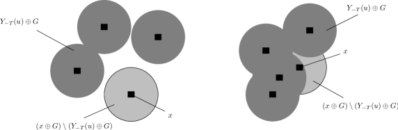
Figure 3.2: Another look at Figure 3.1 with some shading added to show the process of simulation. Dark shading shows $Y_{-T}(u)\oplus G$ where $Y_{-T}(u)$ is the state of either $U$ or $L$ immediately before we add the new event and $G$ could be either $G_{1}$ or $G_{2}$. Light shading shows the amount added if we accept the new event. In the configuration on the left, $x\oplus G=(x\oplus G)\setminus(Y_{-T}(u)\oplus G)$, so that the attractive term in (3.4) or (3.5) will be very small, whereas the repulsive term will be large. In the configuration on the right we are adding very little area to $(Y_{-T}(u)\oplus G)$ by adding the event, so the attractive term will be larger and the repulsive term will be smaller.

4 Redwood seedlings data

Figure 3.3: Redwood seedlings data. Left: The data, selected by Ripley, (1977) from a larger data set analysed by Strauss, (1975). Right: Plot of the point-process L-function for the redwood seedlings. There seems to be interaction at 3 different scales: (very) small scale repulsion followed by attraction at a moderate scale and then repulsion at larger scales.

We take a brief look at a data set which has been much analysed in the literature, the Redwood seedlings data first considered by Strauss, (1975). We examine a subset of the original data chosen by Ripley, (1977) and later analysed by Diggle, (1978) among others. The data are plotted in Figure 3.3. We wish to model these data using the multiscale model we have introduced. The right pane of Figure 3.3 gives the estimated point process L-function of the data, defined by $L(t)=\sqrt{\pi^{-1}K(t)}$ where $K$ is the K-function as defined by Ripley, (1976, 1977).

From this plot we estimate values of $R_{1}$ and $R_{2}$ as $0.07$ and $0.013$ respectively, giving repulsion at small scales and attraction at moderate scales. It also seems that there is some repulsion at slightly larger scales, so it may be possible to use $R_{2}=0.2$ and to model the large-scale interaction rather than the small-scale interaction as we have chosen.

Figure 3.4: Point process L- and transformed T-function plots of the redwood seedlings data. Left: L-function plots of the data together with simulations of the multiscale model with parameters $R_{1}=0.07$, $R_{2}=0.013$, $\lambda=0.118$, $\gamma_{1}=2000$ and $\gamma_{2}=10^{-200}$. Dotted lines give an envelope of 19 simulations of the model, the solid line is the redwood seedlings data and the dashed line is the average of the 19 simulations. Right: the corresponding plots for the transformed T-function.

Experimenting with various values for the remaining parameters, we chose values $\gamma_{1}=2000$ and $\gamma_{2}=10^{-200}$. The value $\lambda=0.118$ was chosen to give about 62 points in each realisation, the number in the observed data set. The remarkably small value of $\gamma_{2}$ was necessary because the value of $R_{2}$ was also very small. It is clear from these numbers that it would be more natural to define $\gamma_{1}$ and $\gamma_{2}$ on a logarithmic scale. Figure 3.4 shows point process L- and T-function plots for 19 simulations from this model, providing approximate 95% Monte-Carlo confidence envelopes for the values of the functions. It can be seen that on the basis of these functions, the model appears to fit the data reasonably well. The T-function, defined by Schladitz and Baddeley, (2000), is a third order analogue of the K-function, and for a Poisson process $T(r)$ is proportional to $r^{4}$; in Figure 3.4 the function is transformed by taking the fourth root of a suitable multiple and then subtracting $r$, in order to yield a function whose theoretical value for a Poisson process would be zero.

The plots show several things: firstly that the model fits reasonably well, but that it is possible that we chose a value of $R_{1}$ which was slightly too large. Perhaps $R_{1}=0.06$ would have been better. Secondly, it seems that the large-scale repulsion may be an important factor which should not be ignored. Thirdly, in this case we have gained little new information by plotting the T-function—the third-order behaviour of the data seems to be similar in nature to the second-order structure.

5 Further comments

The main advantage of our method for the perfect simulation of locally stable point processes is that it allows acceptance probabilities to be computed in $O(n)$ instead of $O(2^{n})$ steps for models which are neither purely attractive nor purely repulsive. Because of the exponential dependence on $n$, the algorithm of Kendall and Møller, (2000) is not feasible in these situations.

It is clear that in practice it is possible to extend the work to more general multiscale models. For example, the sample $L$-function of the redwood seedlings might, if the sample size were larger, indicate the appropriateness of a three-scale model

$$p(X)=\alpha\lambda^{N(X)}\gamma_{1}^{-m(X\oplus G_{1})}\gamma_{2}^{-m(X\oplus G_{2})}\gamma_{3}^{-m(X\oplus G_{3})}.$$ (3.6)

The proof given in the Appendix of Ambler and Silverman, (2004b) can easily be extended to show the existence of this process, and (3.6) is also amenable to perfect simulation using the method of Section 3. Because of the small size of the redwood seedlings data set a model of this complexity is not warranted, but the fitting of such models, and even higher order multiscale models in appropriate circumstances, would be an interesting topic for future research.

Another topic is the possibility of fitting parameters by a more systematic approach than the subjective adjustment approach we have used. Ambler and Silverman, (2004b) set out the possibility of using pseudo-likelihood (Besag,, 1974, 1975, 1977; Jensen and Møller,, 1991) to estimate the parameters $\lambda$, $\gamma_{1}$ and $\gamma_{2}$ for given $R_{1}$ and $R_{2}$. However, this method has yet to be implemented and investigated in practice.

4 Nonparametric regression by wavelet thresholding

1 Introductory remarks

We now turn to our next theme, nonparametric regression. Suppose we observe

$$y_{i}=g(t_{i})+\varepsilon_{i}.$$ (4.1)

where $g$ is an unknown function sampled with error at regularly spaced intervals $t_{i}$. The noise, $\varepsilon_{i}$ is assumed to be independent and Normally distributed with zero mean and variance $\sigma^{2}$.

The standard wavelet-based approach to this problem is based on two properties of the wavelet transform:

1. A large class of ‘well-behaved’ functions can be sparsely represented in wavelet space;

2. The wavelet transform maps independent identically distributed noise to independent identically distributed wavelet coefficients.

These two properties combine to suggest that a good way to remove noise from a signal is to transform the signal into wavelet space, discard all of the small coefficients (i.e. threshold), and perform the inverse transform. Since the true (noiseless) signal had a sparse representation in wavelet space, the signal will essentially be concentrated in a small number of large coefficients. The noise, on the other hand, will still be spread evenly among the coefficients, so by discarding the small coefficients we must have discarded mostly noise and will thus have found a better estimate of the true signal.

The problem then arises of how to choose the threshold value. General methods that have been applied in the wavelet context are SureShrink (Donoho and Johnstone,, 1995), cross-validation (Nason,, 1996) and false discovery rates (Abramovich and Benjamini,, 1996). In the BayesThresh approach (Abramovich et al.,, 1998) proposes a Bayesian hierarchical model for the wavelet coefficients, using a mixture of a point mass at $0$ and a $N(0,\tau^{2})$ density as their prior. The marginal posterior median of the population wavelet coefficient is then used as the estimate. This gives a thresholding rule, since the point mass at $0$ in the prior gives non-zero probability that the population wavelet coefficient will be zero.

Most Bayesian approaches to wavelet thresholding model the coefficients independently. In order to capture the notion that nonzero wavelet coefficients may be in some way clustered, we allow prior dependency between the coefficients by modelling them using an extension of the area-interaction process as defined in Section 1 above. The basic idea is that if a coefficient is nonzero then it is more likely that its neighbours (in a suitable sense) are also non-zero. We then use an appropriate CFTP approach to sample from the posterior distribution of our model.

2 A Bayesian model for wavelet thresholding

Abramovich et al., (1998) consider the problem where the true wavelet coefficients are observed subject to Gaussian noise with zero mean and some variance $\sigma^{2}$,

$$\widehat{d}_{jk}|d_{jk}\sim N(d_{jk},\sigma^{2}),$$

where $\widehat{d}_{jk}$ is the value of the noisy wavelet coefficient (the data) and $d_{jk}$ is the value of the true (noiseless) coefficient.

Their prior distribution on the true wavelet coefficients is a mixture of a Normal distribution with zero mean and variance dependent on the level of the coefficient, and a point mass at zero as follows:

$$d_{jk}\sim\pi_{j}N(0,\tau_{j}^{2})+(1-\pi_{j})\delta(0),$$ (4.2)

where $d_{jk}$ is the value of the $k$th coefficient at level $j$ of the discrete wavelet transform, and the mixture weights $\{\pi_{j}\}$ are constant within each level. An alternative formulation of this can be obtained by introducing auxiliary variables $Z=\{\zeta_{jk}\}$ with $\zeta_{jk}\in\{0,1\}$ and independent hyperpriors

$$\zeta_{jk}\sim\text{Bernoulli}(\pi_{j}).$$ (4.3)

The prior given in equation (4.2) is then expressed as

$$d_{jk}|Z\sim N(0,\zeta_{jk}\tau_{j}^{2}).$$ (4.4)

The starting point for our extension of this approach is to note that $Z$ can be considered to be a point process on the discrete space, or lattice, $\chi$ of indices $(j,k)$ of the wavelet coefficients. The points of $Z$ give the locations at which the prior variance of the wavelet coefficient, conditional on $Z$, is nonzero. From this point of view, the hyperprior structure given in equation (4.3) is equivalent to specifying $Z$ to be a Binomial process with rate function $p(j,k)=\pi_{j}$.

Our general approach will be to replace $Z$ by a more general lattice process $\xi$ on $\chi$. We allow $\xi$ to have multiple points at particular locations $(j,k)$, so that the number $\xi_{jk}$ of points at $(j,k)$ will be a non-negative integer, not necessarily confined to $\{0,1\}$. We will assume that the prior variance is proportional to the number of points of $\xi$ falling at the corresponding lattice location. So if there are no points, the prior will be concentrated at zero and the corresponding observed wavelet will be treated as pure noise; on the other hand, the larger the number of points, the larger the prior variance and the less shrinkage applied to the observed coefficient. To allow for this generalisation, we extend (4.4) in the natural way to

$$d_{jk}|\xi\sim N(0,\tau^{2}\xi_{jk}),$$ (4.5)

where $\tau^{2}$ is a constant.

We now consider the specification of the process $\xi$. While it is reasonable that the wavelet transform will produce a sparse representation, the time-frequency localisation properties of the transform also make it natural to expect that the representation will be clustered in some sense. The existence of this clustered structure can be seen clearly in Figure 4.1, which shows the discrete wavelet transform of several common test functions represented in the natural binary tree configuration.

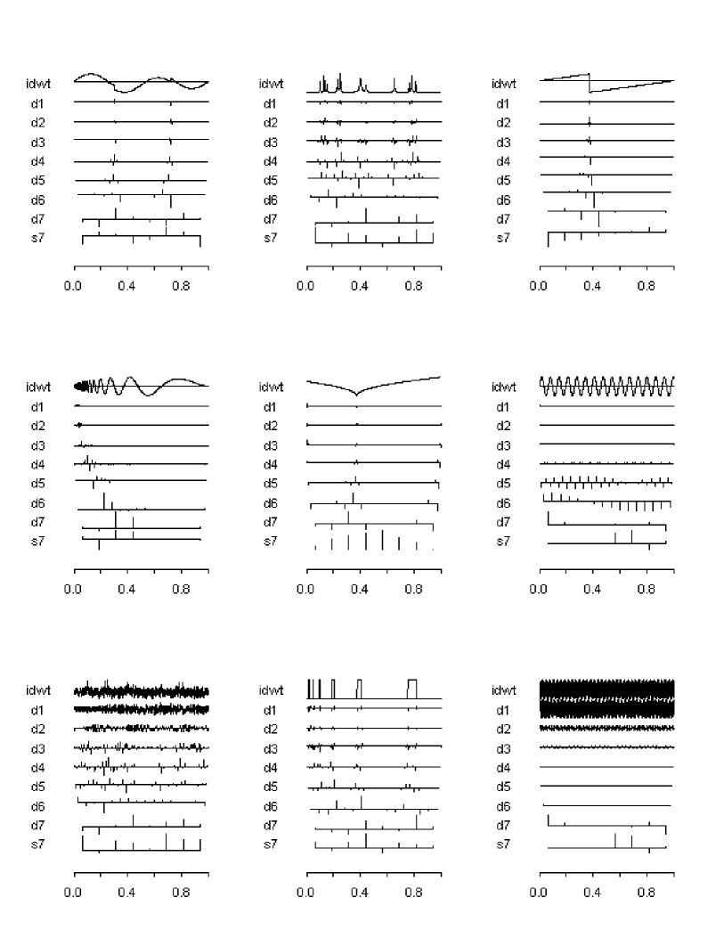
Figure 4.1: Examples of the discrete wavelet transform of some test functions. There is clear evidence of clustering in most of the graphs. The original functions are shown above their discrete wavelet transform each time.

With this clustering in mind, we model $\xi$ as an area-interaction process on the space $\chi$. The choice of the neighbourhoods $B(x)$ for $x$ in $\chi$ will be discussed below. Given the choice of neighbourhoods, the process will be defined by

$$p(\xi)=\alpha\lambda^{N(\xi)}\gamma^{-m\{U(\xi)\}}$$ (4.6)

where $p(\xi)$ is the intensity relative to the unit rate independent auto-Poisson process (Cressie,, 1993). If we take $\gamma>1$ this gives a clustered configuration. Thus we would expect to see clusters of large values of $d_{jk}$ if this were a reasonable model—which is exactly what we do see in Figure 4.1.

A simple application of Bayes’s theorem tells us that the posterior for our model is

$$p(\xi,\mathbf{d}|\widehat{\mathbf{d}})=p(\xi)\prod_{j,k}p(d_{jk}|\xi_{jk})\prod_{j,k}p(\widehat{d}_{jk}|d_{jk},\xi_{jk})$$ (4.7)

$$= \alpha\lambda^{N(\xi)}\gamma^{-m\{U(\xi)\}}\prod_{j,k}\frac{\exp(-d_{jk}^{2}/2\tau^{2}\xi_{jk})}{\sqrt{2\pi\tau^{2}\xi_{jk}}}\prod_{j,k}\frac{\exp\{-(\widehat{d}_{jk}-d_{jk})^{2}/2\sigma^{2}\}}{\sqrt{2\pi\sigma^{2}}}$$

$$= \alpha\lambda^{N(\xi)}\gamma^{-m\{U(\xi)\}}\prod_{j,k}\frac{\exp\{-d_{jk}^{2}/2\tau^{2}\xi_{jk}-(\widehat{d}_{jk}-d_{jk})^{2}/2\sigma^{2}\}}{\sqrt{2\pi\tau^{2}\xi_{jk}}\sqrt{2\pi\sigma^{2}}}.$$

Clearly (4.7) is not a standard density. In Section 1 we show how the extension of the coupling-from-the-past algorithm described in Section 3 enables us to sample from it.

3 Completing the specification

We first note that in this context $\chi$ is a discrete space, so the technical conditions required in Section 1 of $m(\cdot)$ and $B(\cdot)$ are trivially satisfied.

In order to complete the specification of our area-interaction prior for $\xi$, we need a suitable interpretation of the neighbourhood of a location $x=(j,k)$ on the lattice $\chi$ of indices $(j,k)$ of wavelet coefficients. This lattice is a binary tree, and there are many possibilities. We decided to use the parent, the coefficient on the parent’s level of the transform which is next-nearest to $x$, the two adjacent coefficients on the level of $x$, the two children and the coefficients adjacent to them, making a total of nine coefficients (including $x$ itself). Figure 4.2 illustrates this scheme, which captures the localisation of both time and frequency effects. Figure 4.2 also shows how we dealt with boundaries: we assume that the signal we are examining is periodic, making it natural to have periodic boundary conditions in time.

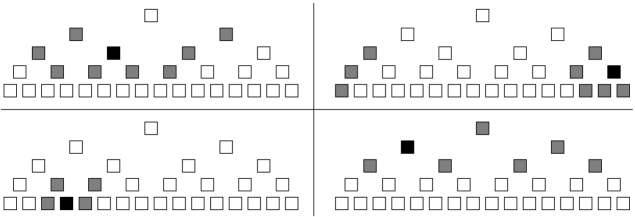
Figure 4.2: The four plots give examples of what we used as $B(\cdot)$ for four different example locations showing how we dealt with boundaries. Grey boxes are $B(x)\setminus\{x\}$ for each example location $x$, while $x$ itself is shown as black.

If $B(x)$ overlaps with a frequency boundary we simply discard those parts which have no locations associated with them. The simple counting measure used has $m\{B(x)\}=9$ unless $x$ is in the bottom row or one of the top two rows.

Other possible neighbourhood functions include using only the parent, children and immediate sibling and cousin of a coefficient as $B(x)$, or a variation on this taking into account the length of support of the wavelet used. Though we have chosen to use periodic boundary conditions, our method is equally applicable without this assumption, with appropriate modification of $B(x)$.

5 Perfect simulation for wavelet curve estimation

1 Exact posterior sampling for lattice processes

In this section, we develop a practical approach to simulation from a close approximation to the posterior density (4.7), making use of coupling from the past. One of the advantages of the Normal model we propose in Section 2 is that it is possible to integrate out $d_{jk}$ and work only with the lattice process $\xi$. Performing this calculation, we see that equation (4.7) can be rewritten as

$$p(\xi|\widehat{\mathbf{d}})=p(\xi)\prod_{j,k}\frac{\exp\left\{-\widehat{d}_{jk}^{2}/2(\sigma^{2}+\tau^{2}\xi_{jk})\right\}}{\sqrt{2\pi(\sigma^{2}+\tau^{2}\xi_{jk})}},$$

by the standard convolution properties of normal densities. We now see that it is possible to sample from the posterior by simulating only the process $\xi$ and ignoring the marks $\mathbf{d}$. This lattice process is amenable to perfect simulation using the method of Section 3 above. Let

$$f_{1}(\xi)= \;\lambda^{N(\xi)},$$

$$f_{2}(\xi)= \;\gamma^{-m\left\{U(\xi)\right\}},$$

$$f_{3}(\xi)= \;\prod_{j,k}\exp\{-\widehat{d}_{jk}^{2}\left/\right.2(\sigma^{2}+\tau^{2}\xi_{jk})\}\text{ and}$$

$$f_{4}(\xi)= \;\prod_{j,k}\left\{2\pi(\sigma^{2}+\tau^{2}\xi_{jk})\right\}^{-1/2}.$$

Then

$$\lambda_{f_{1}}(u;\xi)= \;\lambda,$$

$$\lambda_{f_{2}}(u;\xi)= \;\gamma^{-m\left\{B(u)\setminus U(\xi)\right\}}\leq 1,$$

$$\lambda_{f_{3}}(u;\xi)= \;\exp\left\{\frac{\widehat{d}_{u}^{2}\tau^{2}}{2(\sigma^{2}+\tau^{2}\xi_{u})\{\sigma^{2}+\tau^{2}(\xi_{u}+1)\}}\right\}$$

$$\>\leq\exp\left\{\frac{\widehat{d}_{u}^{2}\tau^{2}}{2\sigma^{2}(\tau^{2}+\sigma^{2})}\right\}\text{ and}$$

$$\lambda_{f_{4}}(u;\xi)= \;\left\{\frac{\tau^{2}\xi_{u}+\sigma^{2}}{\tau^{2}(\xi_{u}+1)+\sigma^{2}}\right\}^{1/2}\leq 1.$$

By a slight abuse of notation, in the second and third equations above we use $u$ to refer both to the point $\{u\}$ and the location $(j,k)$ at which it is found. The functions $f_{1}$, …, $f_{4}$ are also monotone with respect to the subset relation, so all of the conditions for exact simulation using the method of Section 3 are satisfied.

In the spatial processes considered in detail in Section 3, the dominating process had constant intensity across the space $\chi$. In the present context, however, it is necessary in practice to use a dominating process which has a different rate at each lattice location, and then use location-specific maxima and minima rather than global maxima and minima. Because we can now use location-specific, rather than global, maxima and minima, we can initialise upper and lower processes that are much closer together than would have been possible with a constant-rate dominating process. This has the consequence of reducing coalescence times to feasible levels. A constant-rate dominating process would not have been feasible due to the size of the global maxima, so this modification to the method of Section 3 is essential; see Section 3 for details. Chapter 5 of Ambler, (2002) gives some other examples of dominating processes with location-specific intensities.

The location-specific rate of the dominating process $D$ is

$$\lambda_{jk}^{dom}=\lambda e^{\widehat{d}_{jk}^{2}\tau^{2}/2\sigma^{2}(\tau^{2}+\sigma^{2})}$$ (5.1)

for each location $(j,k)$ on the lattice. The lower process is then started as a thinned version of $D$. Points are accepted with probability

$$P(x)=\gamma^{-M(\chi)}\left(\frac{\sigma^{2}}{\tau^{2}+\sigma^{2}}\right)^{1/2}\times\exp\left\{-\frac{\widehat{d}_{x}^{2}\tau^{2}}{2\sigma^{2}(\tau^{2}+\sigma^{2})}\right\},$$

where $M(\chi)=\max_{\chi}[m\{B(x)\}]$. The upper and lower processes are then evolved through time, accepting points as described in Section 3 with probability

$$\frac{1}{\lambda_{jk}^{dom}}\lambda_{f_{1}}(u;\xi^{\text{up}})\lambda_{f_{2}}(u;\xi^{\text{up}})\lambda_{f_{3}}(u;\xi^{\text{low}})\lambda_{f_{4}}(u;\xi^{\text{up}})$$

for the upper process and

$$\frac{1}{\lambda_{jk}^{dom}}\lambda_{f_{1}}(u;\xi^{\text{low}})\lambda_{f_{2}}(u;\xi^{\text{low}})\lambda_{f_{3}}(u;\xi^{\text{up}})\lambda_{f_{4}}(u;\xi^{\text{low}})$$

for the lower process. The remainder of the algorithm carries over in the obvious way. There are still some issues to be addressed due to very high birth rates in the dominating process, and this will be done in Section 3.

2 Using the generated samples

Although $\mathbf{d}$ was integrated out for simulation reasons in Section 2 it is, naturally, the quantity of interest. Having simulated realisations of $\xi|\widehat{\mathbf{d}}$ we then generate $\mathbf{d}|\xi,\widehat{\mathbf{d}}$ for each realisation $\xi$ generated in the first step. The sample median of $\mathbf{d}|\xi,\widehat{\mathbf{d}}$ gives an estimate for $\mathbf{d}$. The median is used instead of the mean as this gives a thresholding rule, defined by Abramovich et al., (1998) as a rule giving $p(d_{jk}=0|\widehat{\mathbf{d}})>0$.

We calculate $p(\mathbf{d}|\xi,\widehat{\mathbf{d}})$ using logarithms for ease of notation. Assuming that $\xi_{jk}\neq 0$ we find

$$\log p(d_{jk}|\widehat{d}_{jk},\xi_{jk}\neq 0) = \log{p(d_{jk}|\xi_{jk}\neq 0)}+\log{p(\widehat{d}_{jk}|d_{jk},\xi_{jk}\neq 0)}+C$$

$$= \frac{-d_{jk}^{2}}{2\tau^{2}\xi_{jk}}+\frac{-(\widehat{d}_{jk}-d_{jk})^{2}}{2\sigma^{2}}+C_{1}$$

$$= -\frac{(\sigma^{2}+\tau^{2}\xi_{jk})\left(d_{jk}-\frac{\tau^{2}\xi_{jk}\widehat{d}_{jk}}{\sigma^{2}+\tau^{2}\xi_{jk}}\right)^{2}}{2\sigma^{2}\tau^{2}\xi_{jk}}+C_{2}$$

where $C$, $C_{1}$ and $C_{2}$ are constants. Thus

$$d_{jk}|\widehat{d}_{jk},\xi_{jk}\neq 0\sim N\left(\frac{\tau^{2}\xi_{jk}\widehat{d}_{jk}}{\sigma^{2}+\tau^{2}\xi_{jk}},\frac{\sigma^{2}\tau^{2}\xi_{jk}}{\sigma^{2}+\tau^{2}\xi_{jk}}\right).$$

When $\xi_{jk}=0$ we clearly have $p(d_{jk}|\xi_{jk},\widehat{d}_{jk})=0$.

3 Dealing with large and small rates

We now deal with some approximations which are necessary to allow our algorithm to be feasible computationally. Recall from equation (5.1) that if the maximum data value $d_{jk}$ is twenty times larger in magnitude than the standard deviation of the noise (a not uncommon event for reasonable noise levels) then we have

$$\lambda_{dom} = \lambda e^{400\sigma^{2}\tau^{2}/2\sigma^{2}(\tau^{2}+\sigma^{2})}$$

$$= \lambda e^{200\tau^{2}/(\tau^{2}+\sigma^{2})}.$$

Now unless $\tau$ is significantly smaller than $\sigma$, this will result in enormous birth rates, which make it necessary to modify the algorithm appropriately. To address this issue, we noted that the chances of there being no live points at a location whose data value is large (resulting in a value of $\lambda_{dom}$ larger than $e^{4}$) is sufficiently small that for the purposes of calculating $\lambda_{f_{2}}(u;\xi)$ for nearby locations it can be assumed that the number of points alive was strictly positive.

This means that we do not know the true value of $\xi_{jk}$ for the locations with the largest values of $d_{jk}$. This leads to problems since we need to generate $d_{jk}$ from the distribution

$$d_{jk}|\xi_{jk},\widehat{d}_{jk}\sim N\left(\frac{\tau^{2}\xi_{jk}\widehat{d}_{jk}}{\sigma^{2}+\tau^{2}\xi_{jk}},\frac{\sigma^{2}\tau^{2}\xi_{jk}}{\sigma^{2}+\tau^{2}\xi_{jk}}\right),$$

which requires values of $\xi_{jk}$ for each location $(j,k)$ in the configuration. To deal with this issue, we first note that, as $\xi_{jk}\to\infty$,

$$\frac{\tau^{2}\xi_{jk}\widehat{d}_{jk}}{\sigma^{2}+\tau^{2}\xi_{jk}}\hskip 5.0pt\longrightarrow\hskip 5.0pt\widehat{d}_{jk}$$

monotonically from below, and

$$\frac{\tau^{2}\xi_{jk}\sigma^{2}}{\sigma^{2}+\tau^{2}\xi_{jk}}\hskip 5.0pt\longrightarrow\hskip 5.0pt\sigma^{2},$$

also monotonically from below. Since $\sigma$ is typically small, convergence is very fast indeed. Taking $\tau=\sigma$ as an example we see that even when $\xi_{jk}=5$ we have

$$\frac{\tau^{2}\xi_{jk}\widehat{d}_{jk}}{\sigma^{2}+\tau^{2}\xi_{jk}}=\frac{5}{6}\widehat{d}_{jk}$$

and

$$\frac{\tau^{2}\xi_{jk}\sigma^{2}}{\sigma^{2}+\tau^{2}\xi_{jk}}=\frac{5}{6}\sigma^{2}.$$

We see that we are already within $\frac{1}{6}$ of the limit. Convergence is even faster for larger values of $\tau$.

We also recall that the dominating process gives an upper bound for the value of $\xi_{jk}$ at every location. Thus a good estimate for $d_{jk}$ would be gained by taking the value of $\xi_{jk}$ in the dominating process for those points where we do not know the exact value. This is a good solution but is unnecessary in some cases, as sometimes the value of $\lambda_{dom}$ is so large that there is little advantage in using this value. Thus for exceptionally large values of $\lambda_{dom}$ we simply use $N(\widehat{d}_{jk},\sigma^{2})$ numbers as our estimate of $d_{jk}$.

4 Simulation study

We now present a simulation study of the performance of our estimator relative to several established wavelet-based estimators. Similar to the study of Abramovich et al., (1998), we investigate the performance of our method on the four standard test functions of Donoho and Johnstone, (1994, 1995), namely ‘Blocks’, ‘Bumps’, ‘Doppler’ and ‘Heavisine’. These test functions are used because they exhibit different kinds of behaviour typical of signals arising in a variety of applications.

The test functions were simulated at 256 points equally spaced on the unit interval. The test signals were centred and scaled so as to have mean value $0$ and standard deviation $1$. We then added independent $N(0,\sigma^{2})$ noise to each of the functions, where $\sigma$ was taken as $1/10$, $1/7$ and $1/3$. The noise levels then correspond to root signal-to-noise ratios (RSNR) of $10$, $7$ and $3$ respectively. We performed 25 replications. For our method, we simulated 25 independent draws from the posterior distribution of the $d_{jk}$ and used the sample median as our estimate, as this gives a thresholding rule. For each of the runs, $\sigma$ was set to the standard deviation of the noise we added, $\tau$ was set to $1.0$, $\lambda$ was set to $0.05$ and $\gamma$ was set to $3.0$.

The values of parameters $\sigma$ and $\tau$ were set to the true values of the standard deviation of the noise and the signal, respectively. In practice it will be necessary to develop some method for estimating these values. The value of $\lambda$ was chosen to be $0.05$ because it was felt that not many of the coefficients would be significant. The value of $\gamma$ was chosen based on small trials for the heavisine and jumpsine datasets.

We compare our method with several established wavelet-based estimators for reconstructing noisy signals: SureShrink (Donoho and Johnstone,, 1994), two-fold cross-validation as applied by Nason, (1996), ordinary BayesThresh (Abramovich et al.,, 1998), and the false discovery rate as applied by Abramovich and Benjamini, (1996).

For test signals ‘Bumps’, ‘Doppler’ and ‘Heavisine’ we used Daubechies’ least asymmetric wavelet of order 10 (Daubechies,, 1992). For the ‘Blocks’ signal we used the Haar wavelet, as the original signal was piecewise constant. The analysis was carried out using the freely available $R$ statistical package. The WaveThresh package (Nason,, 1993) was used to perform the discrete wavelet transform and also to compute the SureShrink, cross-validation, BayesThresh and false discovery rate estimators.

Table 5.1: Average mean-square errors ($\times 10^{4}$) for the area-interaction BayesThresh (AIBT), SureShrink (SS), cross-validation (CV), ordinary BayesThresh (BT) and false discovery rate (FDR) estimators for four test functions for three values of the root signal-to-noise ratio. Averages are based on 25 replicates. Standard errors are given in parentheses.

RSNR	Method	Test functions
		Blocks		Bumps		Doppler		Heavisine
	AIBT	25	(1)	84	(2)	49	(1)	32	(1)
	SS	49	(2)	131	(6)	54	(2)	66	(2)
10	CV	55	(2)	392	(21)	112	(5)	31	(1)
	BT	344	(10)	1651	(17)	167	(5)	35	(2)
	FDR	159	(14)	449	(17)	145	(5)	64	(3)
	AIBT	56	(3)	185	(5)	87	(3)	52	(2)
	SS	98	(3)	253	(10)	99	(4)	94	(4)
7	CV	96	(3)	441	(25)	135	(6)	54	(3)
	BT	414	(11)	1716	(21)	225	(6)	57	(2)
	FDR	294	(18)	758	(27)	253	(9)	93	(4)
	AIBT	535	(21)	1023	(15)	448	(18)	153	(6)
	SS	482	(13)	973	(45)	399	(14)	147	(3)
3	CV	452	(11)	914	(34)	375	(13)	148	(6)
	BT	860	(24)	2015	(37)	448	(12)	140	(4)
	FDR	1230	(52)	2324	(88)	862	(31)	148	(3)

The goodness of fit of each estimator was measured by its average mean-square error (AMSE) over the 25 replications. Table 5.1 presents the results. It is clear that our estimator performs extremely well with respect to the other estimators when the signal-to-noise ratio is moderate or large, but less well, though still competitively, when there is a small signal-to-noise ratio.

5 Remarks and directions for future work

Our procedure for Bayesian wavelet thresholding has used the naturally clustered nature of the wavelet transform when deciding how much weight to give coefficient values. In comparisons with other methods, our approach performed very well for moderate and low noise levels, and reasonably competitively for higher noise levels.

One possible area for future work would be to replace equation (4.5) with

$$d_{jk}|\xi\sim N(0,\tau^{2}(\xi_{jk})^{z}),$$

where $z$ would be a further parameter. This would modify the number of points which are likely to be alive at any given location and thus also modify the tail behaviour of the prior. The idea behind this suggestion is that when we know that the behaviour of the data is either heavy or light tailed, we could adjust $z$ to compensate. This could possibly also help speed up convergence by reducing the number of points at locations with large values of $d_{jk}$.

A second possible area for future work would be to develop some automatic methods for choosing the parameter values, perhaps using the method of maximum pseudo-likelihood (Besag,, 1974, 1975, 1977).

Finally, it would be of obvious interest to find an approach which made the approximations of Section 3 unnecessary and allowed for true CFTP to be preserved.

6 Conclusion

This paper, based on Ambler and Silverman, (2004a, b), has drawn together a number of themes which demonstrate the way that modern computational statistics has made use of work in applied probability and stochastic processes in ways which would have been inconceivable not many decades ago. It is therefore a particular pleasure to dedicate it to John Kingman on his birthday!

References

- Abramovich and Benjamini, (1996) Abramovich, F., and Benjamini, Y. 1996. Adaptive thresholding of wavelet coefficients. Comput. Statist. Data Anal., 22, 351–361.
- Abramovich et al., (1998) Abramovich, F., Sapatinas, T., and Silverman, B. W. 1998. Wavelet thresholding via a Bayesian approach. J. Roy. Statist. Soc. Ser. B, 60, 725–749.
- Ambler, (2002) Ambler, G. K. 2002. Dominated Coupling from the Past and Some Extensions of the Area-Interaction Process. Ph.D. thesis, Department of Mathematics, University of Bristol.
- Ambler and Silverman, (2004a) Ambler, G. K., and Silverman, B. W. 2004a. Perfect Simulation for Bayesian Wavelet Thresholding with Correlated Coefficients. Tech. rept. Department of Mathematics, University of Bristol. http://arXiv.org/abs/0903.2654v1 [stat.ME].
- Ambler and Silverman, (2004b) Ambler, G. K., and Silverman, B. W. 2004b. Perfect Simulation of Spatial Point Processes using Dominated Coupling from the Past with Application to a Multiscale Area-Interaction Point Process. Tech. rept. Department of Mathematics, University of Bristol. http://arXiv.org/abs/0903.2651v1 [stat.ME].
- Baddeley and Lieshout, (1995) Baddeley, A. J., and Lieshout, M. N. M. van. 1995. Area-interaction point processes. Ann. Inst. Statist. Math., 47, 601–619.
- Baddeley et al., (2005) Baddeley, A. J., Turner, R., Møller, J., and Hazelton, M. 2005. Residual analysis for spatial point processes (with Discussion). J. Roy. Statist. Soc. Ser. B, 67, 617–666.
- Besag, (1974) Besag, J. E. 1974. Spatial interaction and the statistical analysis of lattice systems. J. Roy. Statist. Soc. Ser. B, 36, 192–236.
- Besag, (1975) Besag, J. E. 1975. Statistical analysis of non-lattice data. The Statistician, 24, 179–195.
- Besag, (1977) Besag, J. E. 1977. Some methods of statistical analysis for spatial data. Bull. Int. Statist. Inst., 47, 77–92.
- Connor, (2007) Connor, S. 2007. Perfect sampling. In: Ruggeri, F., Kenett, R., and Faltin, F. (eds), Encyclopedia of Statistics in Quality and Reliability. New York: John Wiley & Sons.
- Cressie, (1993) Cressie, N. A. C. 1993. Statistics for Spatial Data. New York: John Wiley & Sons.
- Daubechies, (1992) Daubechies, I. 1992. Ten Lectures on Wavelets. Philadelphia, PA: SIAM.
- Diggle, (1978) Diggle, P. J. 1978. On parameter estimation for spatial point processes. J. Roy. Statist. Soc. Ser. B, 40, 178–181.
- Donoho and Johnstone, (1994) Donoho, D. L., and Johnstone, I. M. 1994. Ideal spatial adaption by wavelet shrinkage. Biometrika, 81, 425–455.
- Donoho and Johnstone, (1995) Donoho, D. L., and Johnstone, I. M. 1995. Adapting to unknown smoothness via wavelet shrinkage. J. Amer. Statist. Assoc., 90, 1200–1224.
- Green and Murdoch, (1998) Green, P. J., and Murdoch, D. J. 1998. Exact sampling for Bayesian inference: towards general purpose algorithms (with discussion). Pages 301–321 of: Bernardo, J. M., Berger, J. O., Dawid, A. P., and Smith, A. F. M. (eds), Bayesian Statistics 6. Oxford: Oxford Univ. Press.
- Häggström et al., (1999) Häggström, O., Lieshout, M. N. M. van, and Møller, J. 1999. Characterisation results and Markov chain Monte Carlo algorithms including exact simulation for some spatial point processes. Bernoulli, 5, 641–658.
- Jensen and Møller, (1991) Jensen, J. L., and Møller, J. 1991. Pseudolikelihood for exponential family models of spatial point processes. Ann. Appl. Probab., 1, 445–461.
- Kelly and Ripley, (1976) Kelly, F. P., and Ripley, B. D. 1976. A note on Strauss’s model for clustering. Biometrika, 63, 357–360.
- Kendall, (1997) Kendall, W. S. 1997. On some weighted Boolean models. Pages 105–120 of: Jeulin, D. (ed), Advances in Theory and Applications of Random Sets. Singapore: World Scientific.
- Kendall, (1998) Kendall, W. S. 1998. Perfect simulation for the area-interaction point process. Pages 218–234 of: Accardi, L., and Heyde, C. C. (eds), Probability Towards 2000. New York: Springer-Verlag.
- Kendall and Møller, (2000) Kendall, W. S., and Møller, J. 2000. Perfect simulation using dominated processes on ordered spaces, with applications to locally stable point processes. Adv. in Appl. Probab., 32, 844–865.
- MacKay, (2003) MacKay, D. J. C. 2003. Information Theory, Inference, and Learning Algorithms. Cambridge: Cambridge Univ. Press.
- Matheron, (1975) Matheron, G. 1975. Random Sets and Integral Geometry. New York: John Wiley & Sons.
- Murdoch and Green, (1998) Murdoch, D. J., and Green, P. J. 1998. Exact sampling from a continuous state space. Scand. J. Statist., 25, 483–502.
- Nason, (1993) Nason, G. P. 1993. The WaveThresh Package: Wavelet Transform and Thresholding Software for S-Plus and R. Available from Statlib.
- Nason, (1996) Nason, G. P. 1996. Wavelet shrinkage using cross-validation. J. Roy. Statist. Soc. Ser. B, 58, 463–479.
- Papangelou, (1974) Papangelou, F. 1974. The conditional intensity of general point processes and an application to line processes. Z. Wahrscheinlichkeitstheorie verw. Geb., 28, 207–226.
- Propp and Wilson, (1996) Propp, J. G., and Wilson, D. B. 1996. Exact sampling with coupled Markov chains and applications to statistical mechanics. Random Structures & Algorithms, 9, 223–252.
- Propp and Wilson, (1998) Propp, J. G., and Wilson, D. B. 1998. How to get a perfectly random sample from a generic Markov chain and generate a random spanning tree of a directed graph. J. Algorithms, 27, 170–217.
- Ripley, (1976) Ripley, B. D. 1976. The second-order analysis of stationary point processes. J. Appl. Probab., 13, 255–266.
- Ripley, (1977) Ripley, B. D. 1977. Modelling spatial patterns (with Discussion). J. Roy. Statist. Soc. Ser. B, 39, 172–212.
- Schladitz and Baddeley, (2000) Schladitz, K., and Baddeley, A. J. 2000. A third order point process characteristic. Scand. J. Statist., 27, 657–671.
- Strauss, (1975) Strauss, D. J. 1975. A model for clustering. Biometrika, 62, 467–475.