Peak to Average Power Ratio Reduction for Space-Time Codes That Achieve Diversity-Multiplexing Gain Tradeoff

Abstract

Zheng and Tse have shown that over a quasi-static channel, there exists a fundamental tradeoff, known as the diversity-multiplexing gain (D-MG) tradeoff. In a realistic system, to avoid inefficiently operating the power amplifier, one should consider the situation where constraints are imposed on the peak to average power ratio (PAPR) of the transmitted signal. In this paper, the D-MG tradeoff of multi-antenna systems with PAPR constraints is analyzed. For Rayleigh fading channels, we show that the D-MG tradeoff remains unchanged with any PAPR constraints larger than one. This result implies that, instead of designing codes on a case-by-case basis, as done by most existing works, there possibly exist general methodologies for designing space-time codes with low PAPR that achieve the optimal D-MG tradeoff. As an example of such methodologies, we propose a PAPR reduction method based on constellation shaping that can be applied to existing optimal space-time codes without affecting their optimality in the D-MG tradeoff. Unlike most PAPR reduction methods, the proposed method does not introduce redundancy or require side information being transmitted to the decoder. Two realizations of the proposed method are considered. The first is similar to the method proposed by Kwok except that we employ the Hermite Normal Form (HNF) decomposition instead of the Smith Normal Form (SNF) to reduce complexity. The second takes the idea of integer reversible mapping which avoids the difficulty in matrix decomposition when the number of antennas becomes large. Sphere decoding is performed to verify that the proposed PAPR reduction method does not affect the performance of optimal space-time codes.

EDICS     MSP-STCD

I Introduction

The results in [1] on the diversity-multiplexing gain (D-MG) tradeoff spurred numerous research activities towards the construction of space-time codes achieving the optimal tradeoff [2, 3, 4, 5, 6, 7, 8]. When examining these space-time codes, we find that these codes generally lead to high peak-to-average power ratio (PAPR) on each antenna. In practice, PAPR of the signals transmitted is an important parameter to be considered during hardware design. A high PAPR poses difficulties in the design of the amplifier and raises the cost of the transmitter. These practical issues motivate our study on the D-MG tradeoff of multi-antenna systems with PAPR constraints. For Rayleigh fading channels, our analytical result shows that the D-MG tradeoff remains the same with any PAPR constraints larger than one. To the best of our knowledge, this is the first analytical result in the literature on the D-MG tradeoff of multi-antenna systems with PAPR constraints. This result implies that, instead of designing codes on a case-by-case basis, as done by most existing works (e.g., [9]), there possibly exist general methodologies for designing space-time codes with low PAPR that achieve the optimal D-MG tradeoff. As an example of such methodologies, we propose a PAPR reduction method based on constellation shaping that can be applied to existing optimal space-time codes without affecting their optimality in the D-MG tradeoff. Unlike most PAPR reduction methods, the proposed method does not introduce redundancy or require side information being transmitted to the decoder. In general, constellation shaping can be tailored to serve different purposes (e.g., minimizing the average transmission power) which often result in different shaping regions. The purposes of the proposed method are reduction of PAPR, and not affecting the rate and optimality in the D-MG tradeoff of the original code. For easier implementation and illustration, the target shaping region is a hypercube which will lead to an asymptotic PAPR of $3$ when the constellation size is large. Lower PAPR might be possible with a different shaping region, which, however, might be difficult to implement. A similar approach was proposed in [10, Chapter 5] for PAPR reduction of orthogonal frequency division multiplexing (OFDM) systems with constellation shaping based on the Smith Normal Form (SNF) [11] decomposition of integer matrices. Due to the prohibitive computational complexity of the SNF decomposition when the number of OFDM carriers is large, the author of [10] also considered discrete Hadamard transform (DHT) based multi-channel systems which rendered a low-complexity SNF decomposition. The authors of [12] then took the constellation shaping algorithm derived for DHT-based systems and applied it to OFDM systems, in conjunction with a selective mapping (SLM) method which incurred redundant bits to overcome the residual PAPR problem due to the mismatch in constellation shaping.

Two realizations of the proposed method will be discussed. The first is similar to the one in [10], except that we employ the Hermite Normal Form (HNF) decomposition [13][14] instead of the SNF decomposition to reduce the computational complexity. The second takes the idea of integer reversible mapping [15][16] which avoids the bit assignment problem in the above methods, and the difficulty in integer matrix decomposition when the size of the matrix becomes large. Therefore, this approach is more suitable for the situations where the number of transmit antennas or the number of OFDM carriers is large. Aside from these advantages over the methods in [10] and [12], it is also worth mentioning that our work is better justified because the integer-based constellation shaping is crucial in preserving the optimality of space-time codes, while for the uncoded OFDM application considered in [10] and [12], the integer-based constellation shaping is not necessary, and its advantage over the non-integer-based shaping schemes (for example, the single carrier frequency division multiple access (SC-FDMA) [17] scheme is equivalent to using a discrete Fourier transform (DFT) to shape the constellation) is yet for investigation. Note that the concept and derivation of the proposed method are very general, thus they can be applied to any linear transform based multi-channel modulation. For the space-time codes considered in this paper, simulation results using sphere decoding verify that the proposed PAPR reduction method does not affect the optimality of the codes.

The rest of this paper is organized as follows. Section II introduces the system model and the definitions of diversity and multiplexing gains. In Section III, we analyze the D-MG tradeoff with any PAPR constraint larger than one, and show that, in Rayleigh fading channels, the D-MG tradeoff remains unchanged. In Section IV, a unified framework of approximate cubic shaping is described. In Section V and Section VI, we propose two approaches of PAPR reduction via approximate cubic shaping. The first selects the transmitted signal using the HNF decomposition, while the second takes the idea of integer reversible mapping. Section VII provides some simulation results and discussions. Finally, conclusions are drawn in Section VIII.

II System Model and Definitions

II-A System Model

As in [1], consider a wireless link with $m$ transmit and $n$ receive antennas. The fading coefficient $h_{ij}$ is the path gain from transmit antenna $j$ to receive antenna $i$. Let the channel matrix ${\mathbf{H}}=[h_{ij}]\in\mathbb{C}^{n\times m}$. We assume that the fading coefficients are independent complex Gaussian with zero mean, unit variance, and known to the receiver, but not to the transmitter. We also assume that the channel matrix ${\bf{H}}$ remains constant within a block of $l$ symbols. That is, the block length is much smaller than the coherence time of the channel. Then the channel, within one block, can be written as

$${\bf{Y}}=\sqrt{\frac{{SNR}}{m}}{\bf{HX}}+{\bf{W}}$$ (1)

where ${\mathbf{X}}\in\mathbb{C}^{m\times l}$ has entries $x_{ij}$, $i=1,...,m,j=1,...,l$, being the signals transmitted by antenna $i$ at time $j$ such that the average transmission power on each antenna in each symbol duration is $1$; ${\mathbf{Y}}\in\mathbb{C}^{n\times l}$ is the received signal; ${\mathbf{W}}$ is the additive noise with independent and identically distributed (i.i.d.) entries $w_{ij}\sim\mathbb{C}N(0,1)$ (i.e., complex Gaussian with mean $0$ and variance $1$); $SNR$ is the average signal-to-noise ratio (SNR) at each receive antenna. A codebook ${\bf{C}}$ with rate $R$ bits per second per hertz (b/s/Hz) is used, which has $|{\mathbf{C}}|={2^{Rl}}$ codewords each being an $m\times l$ matrix.

II-B Diversity and Multiplexing Gains

For the case without PAPR constraints on each antenna, in order to achieve a certain fraction of the capacity at high SNR, one should consider a family of codes that support a data rate which increases with $\log(SNR)$. The diversity and multiplexing gains are defined as [1]

Definition 1

A diversity gain $d^{*}(r)$ is achieved at multiplexing gain $r$ if the data rate $R(SNR)$ satisfies

$$\begin{gathered}\mathop{\lim}\limits_{SNR\to\infty}\frac{{R(SNR)}}{{\log SNR}}=r\hfill\\ \end{gathered}$$ (2)

and the outage probability $P_{out}(R)$ satisfies

$$\begin{gathered}\mathop{\lim}\limits_{SNR\to\infty}\frac{{\log P_{out}(R)}}{{\log SNR}}=-d^{*}(r)\hfill\\ \end{gathered}$$ (3)

∎

The function $d^{*}(r)$ characterizes the D-MG tradeoff. For convenience, we borrow the notation introduced in [1] to denote exponential equality. That is, $f(SNR)\doteq SNR^{b}$ means

$$\mathop{\lim}\limits_{SNR\to\infty}\frac{{\log f(SNR)}}{{\log SNR}}=b.$$

$\dot{\geq}$ , $\dot{\leq}$ are similarly defined.

III Diversity-Multiplexing Gain Tradeoff with PAPR constraints

When space-time codes are used in a multi-antenna system, due to the coding procedure which combines the information symbols to form the coded symbols for each transmit antenna, high PAPR values may occur, especially when the number of transmit antennas is large. To reflect the limitations of practical communication systems, we take PAPR into consideration and investigate the effect of PAPR constraints on the D-MG tradeoff.

III-A The Behavior of Capacity at High SNR with PAPR Constraints

For the study on the optimal D-MG tradeoff with PAPR constraints, characterization of the multiplexing gain is needed. That is, we need to know how the capacity grows with SNR. However, the expression of the exact capacity of a multi-antenna channel with inputs subject to average total power and PAPR constraints may not be a closed form, or may be too complicated (for the single antenna scenario with average power and peak power constraints, see [18], [19]). Fortunately, since the D-MG tradeoff is an asymptotic tradeoff, what we need is simply the behavior of the capacity for asymptotically large SNR. In this section, we will derive a lower bound of the capacity with average total power and PAPR constraints. The bound is tight enough for the derivation of the D-MG tradeoff. The capacity without PAPR constraints (already known in [20], [21]) can be used as an upper bound. These two bounds are then used to characterize the capacity for large SNR.

Since the channel remains constant within a block, the capacity achieving signal and average power distribution should not favor one symbol duration over another within the same block. Thus, for the purpose of analyzing the capacity with respect to the average SNR, it suffices to focus on any symbol duration within a block. We take the signal and noise vectors in (1) pertaining to the same symbol duration, and drop the time index to form a new vector channel model

$$\mathbf{y=Hx+w}$$ (4)

where ${\mathbf{x}}\in\mathbb{C}^{m}$ is the transmitted signal vector scaled by the transmission power, ${\mathbf{y}}\in\mathbb{C}^{n}$ is the received signal vector, and the additive noise vector ${\bf{w}}$ has i.i.d. entries $w_{i}\sim\mathbb{C}N(0,1)$. The average total power and PAPR constraints of the transmitted signal ${\bf{x}}$ are ${\bf{P}}>0$ and $\rho_{i}>1$, $i=1,\ldots m$, respectively, such that

$$\mbox{Tr}\left({E_{\mathbf{x}}\left[{{\mathbf{xx}}^{\dagger}}\right]}\right)\leq{\mathbf{P}},$$ (5)

$$\;\;\;\;\;\;\;\;\;\;\;\frac{|x_{i}|^{2}}{{E_{x_{i}}[|x_{i}|^{2}]}}\leq\;\rho_{i},\;\;\;i=1,\ldots m,$$ (6)

where $\mbox{Tr}()$ denotes trace and $\textbf{x}^{\dagger}$ denotes the conjugate transpose of x, $E_{t}[{\;}]$ denotes the expectation with respect to the distribution of $t$, and $x_{i}$ is the $i$-th element of ${\bf{x}}$. With these definitions, we have the following lower bound on the capacity of this channel.

Lemma 1

The ergodic capacity $C$ of the channel (4) with the transmitted signal subject to (5), (6) is:

$$C\geq E_{\mathbf{H}}\left[{\log\det\left({{\mathbf{I}}+\frac{{\mathbf{P}}}{m}{\mathbf{H}}{\mathbf{H}}^{\dagger}}\right)}\right]+\sum\limits_{i=1}^{m}{k_{i}}$$ (7)

where $k_{i}$ are constants defined in Appendix A.

Proof:

The proof is given in Appendix A. ∎

III-B Optimal D-MG Tradeoff with PAPR Constraints

Now we are ready to discuss the D-MG tradeoff with PAPR constraints. We have

Lemma 2

For the Rayleigh fading channel, the ergodic capacity $C$ of the channel (4) with transmitted signal subject to (5), (6) is

$$C\doteq\min(m,n)\log(SNR).$$ (8)

Proof:

Let $C_{\infty}$ be the capacity without PAPR constraints. It is well known that [20][21]

$$\begin{split}C_{\infty}=E_{\mathbf{H}}\left[{\log\det\left({{\mathbf{I}}+\frac{{\mathbf{P}}}{m}{\mathbf{H}}{\mathbf{H}}^{\dagger}}\right)}\right]\doteq\min(m,n)\log(SNR).\end{split}$$

Using $C_{\infty}$ as an upper bound, from (7), we have

$$C_{\infty}+\sum\limits_{i=1}^{m}{k_{i}}\leq C\leq C_{\infty}$$

and clearly,

$$C_{\infty}+\sum\limits_{i=1}^{m}{k_{i}}\doteq\min(m,n)\log(SNR).$$

Thus,

$$C\doteq\min(m,n)\log(SNR).$$

∎

Lemma 2 shows that the multiplexing gain $r$ remains the same even with PAPR constraints. The main result is given in the following theorem.

Theorem 1

For the Rayleigh fading channel, the optimal D-MG tradeoff with any PAPR constraint $\rho>1$ is the same as the case without PAPR constraints .

Proof:

The outage probability is

$$P_{out}(R) =\mathop{\min}\limits_{f_{\mathbf{x}}({\mathbf{x}})}P\left[{I({\mathbf{x}};{\mathbf{y}}|{\mathbf{H}})<R}\right]$$

$$\leq P\left[{\log\det\left({{\mathbf{I}}+\frac{{\mathbf{P}}}{m}{\mathbf{H}}{\mathbf{H}}^{\dagger}}\right)+\sum\limits_{i=1}^{m}{k_{i}}<R}\right]$$

$$\doteq P\left[{\log\det\left({{\mathbf{I}}+SNR{\mathbf{H}}{\mathbf{H}}^{\dagger}}\right)+\sum\limits_{i=1}^{m}{k_{i}}<R}\right]$$ (9)

where $I({\;};{\;})$ denotes the mutual information and $f_{\mathbf{x}}({\mathbf{x}})$ is the probability density function of ${\mathbf{x}}$ subject to equations (5) and (6). The inequality follows from (63) and (9) follows from equation (9) in[1]. Using the same techniques as in [1], denoting $\lambda_{i}$ as the nonzero eigenvalues of ${\mathbf{HH}}^{\dagger}$ and letting $R=r\log SNR$, $\sum\limits_{i=1}^{m}{k_{i}}=K$, $\lambda_{i}=SNR^{-\alpha_{i}}$, $(x)^{+}\triangleq\max(x,0)$, we have

$$P\left[{\left({\log\det\left({SNR{\mathbf{H}}{\mathbf{H^{\dagger}+I}}}\right)+K}\right)<r\log SNR}\right]$$

$$= P\left[\left({\prod\limits_{i=1}^{n}{(1+SNR\lambda_{i})}}\right)<\frac{SNR^{r}}{e^{K}}\right]\;$$

$$\doteq P\left[{\sum\limits_{i=1}^{n}{(1-\alpha_{i})^{+}}<r}\right].\;$$ (10)

Thus $P_{out}(R)\dot{\leq}$ (10) and (10) is exponentially equal to the outage probability without PAPR constraints in [1]. However, the outage probability with PAPR constraints should be larger than the outage probability without PAPR constraints, that is, $P_{out}(R)\dot{\geq}$ (10). Thus $P_{out}(R)\doteq$ (10), and the optimal tradeoff remains the same as the case without PAPR constraints. ∎

Intuitively, this result is not surprising, since the PAPR constraints do not reduce the spatial degree of freedom and the capacity ${C}$ grows like $C_{\infty}$ with increasing SNR.

To show that this optimal tradeoff can be achieved by a code with finite code length, we adopt a similar method as in [1] by choosing the input to be a random code drawn from i.i.d distribution (75).

Theorem 2

For $l\geq m+n-1$, in Rayleigh fading channels with any PAPR constraint $\rho>1$, the optimal D-MG tradeoff is achievable.

Proof:

The proof is given in Appendix C. ∎

IV Approximate Cubic Shaping

In this section, we discuss the fundamental concepts of the shaping techniques we use to reduce the PAPR of existing D-MG optimal space-time codes. A constellation generally consists of a set of points on an $l$-dimensional complex lattice, or an $L$-dimensional real lattice $\lambda_{L}$ (where $L=2l$), that are enclosed within a finite region $\xi_{L}$. The boundary of a signal constellation affects the average power and PAPR for a given transmitted data rate. In selecting the signal constellation, one tries to minimize the average power with low PAPR. The $L$-dimensional constellation consisting of all the points enclosed within an $L$-dimensional cube is called cubic shaping, which leads to a PAPR value equal to $3$ when the constellation size approaches infinity. With the same number of points to be transmitted, the reduction in the average transmission power due to the use of a region $\xi_{L}$ as signal constellation instead of a hypercube is referred to as the shaping gain $\eta_{s}$ of $\xi_{L}$. The region that has the smallest average power for a given volume is an $L$-dimensional sphere. Although the sphere shaping gives the best shaping gain, it also results in high PAPR values when $L$ is large. Shaping of multidimensional constellation has been extensively studied previously [22, 23, 24, 25]. For our interest in PAPR reduction, we will focus on the cubic shaping due to its good PAPR value asymptotically equal to $3$.

Consider the shaping on a general space-time code ${\mathbf{X}}$ in the form of

$${\mathbf{x}}={\mathbf{Gs}},\;\;\;\;\;\;{\mathbf{s}}\in\mathbb{Z}^{M},{\mathbf{G}}\in\mathbb{R}^{M\times M}$$ (11)

where ${\bf{x}}$ is an isomorphic vector representation of ${\bf{X}}$, ${\bf{G}}$ is an invertible generator matrix and ${\bf{s}}$ is the vector of information symbols chosen from $M$-dimensional integer lattice $\mathbb{Z}^{M}$. A Quadrature Amplitude Modulation (QAM) constellation is a subset of a scaled integer lattice $\mathbb{Z}^{M}$.

For example, an $m\times m$ D-MG optimal space-time code X proposed in [7] can be expressed in terms of $m$ vectors $\textbf{x}^{(i)}$, $i=1,2,...,m$,

$$\textbf{ x}^{(i)}={\textbf{G}^{(i)}}\textbf{ s}^{(i)}$$

$$\textbf{s}^{(i)}\in{\mathbb{Z}[i]}^{m},\;\textbf{G}^{(i)}\in{\mathbb{C}^{m\times m}}$$

where $\mathbb{Z}[i]$ stands for the Gaussian integers (i.e. $a+bi,a,b\in\mathbb{Z}$) and each $\textbf{ x}^{(i)}$ corresponds to the symbols in the space-time codeword matrix with positions corresponding to the nonzero elements’ positions of $\textbf{B}^{i-1}$, where

$$\textbf{B}=\begin{pmatrix}0&0&\cdots&0&1\\ 1&0&\cdots&0&0\\ 0&1&\cdots&0&0\\ &&\vdots&&\\ 0&0&\cdots&1&0\end{pmatrix}.$$

Note that although these symbols are on different time and different antennas, they have equal average power with respect to all codewords owing to the code structure [7]. For each $\textbf{ s}^{(i)}$, $\textbf{G}^{(i)}$, we can get the isomorphic representation by separating the real and imaginary parts of $\textbf{ s}^{(i)}$ and $\textbf{G}^{(i)}$ as follows,

$${\textbf{ s}^{\prime(i)}}=\begin{pmatrix}\textbf{s}^{(i)}_{Re}\\ \textbf{s}^{(i)}_{Im}\end{pmatrix}$$

and

$$\textbf{G}^{\prime(i)}=\begin{pmatrix}\textbf{G}^{(i)}_{Re}&-\textbf{G}^{(i)}_{Im}\\ \textbf{G}^{(i)}_{Im}&\textbf{G}^{(i)}_{Re}\end{pmatrix}.$$

Then $\textbf{ x}^{\prime(i)}={\textbf{G}^{\prime(i)}}\textbf{ s}^{\prime(i)}$, where $\textbf{s}^{\prime(i)}\in{\mathbb{Z}}^{2m},\;\textbf{G}^{\prime(i)}\in{\mathbb{R}^{2m\times 2m}}$. This is exactly the same form as (11).

Our goal is to shape the transmitted signals such that the constellation region of $\bf{x}$ is cubic. However, as the constellation points of $\bf{x}$ have to be on the lattice that achieves the optimal D-MG tradeoff, the constellation region will not be exactly cubic. The idea is to shape by cosets. Since the information symbol $\bf{s}$’s lattice is more regular (integer lattice) and easier to label, cosets will be found in the domain of $\bf{s}$ using a basis corresponding (approximately) to the cubic basis for $\bf{x}$. The following two steps illustrate how this can be done.

Step 1: Introduce a set of perturbation vectors $U$ such that each $\mathbf{u}\in U$ is a linear combination of vectors ${\mathbf{v}}^{i}$, $i=1\ldots M$

$${\mathbf{u}}=\alpha_{1}{\mathbf{v}}^{1}+\alpha_{2}{\mathbf{v}}^{2}+...+\alpha_{M}{\mathbf{v}}^{M}$$ (12)

where ${\mathbf{\alpha}}=[\alpha_{1},\alpha_{2},...,\alpha_{M}]^{T}\in\mathbb{Z}^{M}$ and ${\mathbf{v}}^{i}$ has the properties that

$$\begin{split}\;\;{\mathbf{Gv}}^{i}&\triangleq{\mathbf{\bar{v}}}^{i},\;\;\;\;i=1,2,...,M\\ {\mathbf{\bar{v}}}^{i}&=\left[{\varepsilon_{1},\varepsilon_{2},...,\mu_{i},...,\varepsilon_{M}}\right]^{T},\;\;|\mu_{i}|>>|\varepsilon_{j}|,\end{split}$$ (13)

and

$$|\mu_{1}|\cong|\mu_{2}|\cong...\cong|\mu_{M}|.$$ (14)

Let $(\mathbf{s}+\mathbf{u}),\forall\mathbf{u}\in U$, be the coset representing the same information.

Step 2: Choose $(\mathbf{s}+\mathbf{u^{*}})$ as the vector of information symbols such that the transmitted signals, ${\mathbf{x}}={\mathbf{G}}({\mathbf{s}}+{\mathbf{u}}^{*})$ consist of an approximate cubic constellation. The possible transmitted signals can be written as

$${\mathbf{G}}({\mathbf{s}}+{\mathbf{u}}) ={\mathbf{Gs}}+{\mathbf{Gu}}={\mathbf{\bar{s}}}+{\mathbf{\bar{u}}}\;$$

$$={\mathbf{\bar{s}}}+(\alpha_{1}{\mathbf{\bar{v}}}^{1}+\alpha_{2}{\mathbf{\bar{v}}}^{2}+...+\alpha_{M}{\mathbf{\bar{v}}}^{M})$$ (15)

where ${\mathbf{\bar{s}}}\triangleq{\mathbf{Gs}}$, ${\mathbf{\bar{u}}}\triangleq{\mathbf{Gu}}$. In this particular set $U$, each ${\mathbf{u}}$ causes relatively large perturbations on certain elements of ${\mathbf{\bar{s}}}$ where the corresponding $\alpha_{i}\neq 0$. If we treat $\varepsilon_{j}$’s as $0$, to put $\mathbf{x}$ in the cubic constellation, ${\mathbf{u}}^{*}$ can be searched accordingly by modulo operations. However, the mapping from $\bf{s}$ to $\bf{x}$ has to be reversible for successful decoding. In other words, these approximations need to be reversible. In the following two sections, we will propose two such mappings for approximate cubic shaping. An approximate hypercube constellation leads to a low PAPR value of 3 when $\varepsilon_{j}$’s are relatively small, i.e., when the constellation is large enough.

V approximate Cubic Shaping via Hermite Normal Form (HNF) Decomposition

Firstly, we need to decide ${\mathbf{v}}^{i},\;i=1,2,...,M$, in (12). Consider a partition ${\text{ }}\mathbb{Z}^{M}/\Lambda$, where the lattice $\Lambda={\mathbf{Q}}\mathbb{Z}^{M}$, and ${\bf{Q}}$ is an $M\times M$ integer matrix such that

$${\text{ }}\;\;\;{\mathbf{GQ}}\cong\sigma{\mathbf{I}}.\;\;\;\;\;\;$$

The approximation is due to the fact that $\mathbf{Q}$ is an integer matrix. If we choose ${\mathbf{v}}^{i}$ as

$${\mathbf{v}}^{i} ={\mathbf{Qe}}^{i}\;$$ (16)

$${\mathbf{e}}^{i}\; =[0_{(1)},...,0_{(i-1)},1_{(i)},0_{(i+1)},...,0_{(M)}]^{T},$$

clearly, ${\mathbf{v}}^{i}$ has the properties (13) and (14) when $\sigma$ is reasonably large. Thus,

$${\mathbf{\bar{v}}}^{i} \triangleq{\mathbf{Gv}}^{i}\;={\mathbf{GQe}}^{i}$$

$$=\;\left[{\varepsilon_{1},\varepsilon_{2},...,\sigma_{i},...,\varepsilon_{M}}\right]^{T},\;\;|\sigma_{i}|>>|\varepsilon_{j}|$$ (17)

$$\cong\sigma{\mathbf{e}}^{i}.$$

Define $U\triangleq{\mathbf{Q}}\mathbb{Z}^{M}$. We can rewrite (15) in terms of coset ${\mathbf{s}}+U$

$${\mathbf{G}}{\text{(}}{\mathbf{s}}+U) ={\mathbf{Gs}}+{\mathbf{GQ}}\mathbb{Z}^{M}$$

$$={\mathbf{\bar{s}}}+{\mathbf{GQ}}\mathbb{Z}^{M}$$

$$\cong{\mathbf{\bar{s}}}+\sigma\mathbb{Z}^{M}.$$ (18)

Approximate cubic shaping can be done by treating $\varepsilon_{j}$’s as $0$ (equivalently, the approximation in (18) as equality), then searching for ${\mathbf{u}}^{*}\in\textbf{Q}\mathbb{{Z}}^{M}$ to put ${\mathbf{x}}$ in the approximate cubic constellation.

A geometric interpretation of this shaping method is that we choose ${\mathbf{s}}+{\mathbf{u}}^{*}$ in a shaped constellation whose boundary is a parallelotope defined along the columns of ${\bf{Q}}$. Thus the signal boundary in the domain of ${\bf{x}}$ translates to an approximate hypercube. In the following, we will describe the shaping process in three parts: (1) determine $\mathbf{Q}$ (2) find the coset leaders (3)put $\mathbf{x}$ in an approximate hypercube, which are derived in a different point of view from similar works proposed in[12] and [10]. Note that [12] and [10] deal with the PAPR of single-antenna OFDM systems but not D-MG optimal space-time coded systems whose transmitted signals need to be on certain lattices.

(1) Determine $\mathbf{Q}$: The number of cosets, $|\det({\mathbf{Q}})|$ (which will manifest in part (2)), must be large enough to support the target number of points we want to transmit. Therefore, let

$$\begin{gathered}\;\;\;\;\;\;\;\;\;\;\;\;\;\;\;\;{\mathbf{Q}}=\left[{\tilde{\sigma}{\mathbf{G}}^{-1}}\right]\hfill\\ \;\;\;\;\;\;\;\;\;\;\;\;\;\;\;\;\;|\det({\mathbf{Q}})|\geq\sigma^{M}\hfill\\ \end{gathered}$$

where $\left[{\;}\right]$ denotes rounding, which makes the set of perturbation vectors ${\bf{u}}$ belong to the integer lattice $\mathbb{Z}^{M}$, and $|\det({\mathbf{Q}})|$ is the volume of the parallelotope defined by ${\bf{Q}}$, or equivalently, the number of points in the parallelotope. $\sigma^{M}$ is the number of transmitted points. The parameter $\tilde{\sigma}$ should be chosen to be the smallest value that ensures the number of points in the shaped constellation larger than the number of points in the unshaped constellation, so no information will be lost. For the case we concern, $\mathbf{Q}$ can always be chosen as a nonsingular matrix when $\tilde{\sigma}$ is large enough.

(2) Find the coset leaders : The coset leaders ${\bf{s}}$ must satisfy

$$\begin{gathered}\;\;\;\;\;\;\;\mbox{if}\;\;\;{\mathbf{s}}^{i}\neq{\mathbf{s}}^{j}\;\;\;\;\;\;\;\;\;\;\;\;\;\;\hfill\\ \;\;\;\mbox{then}\;\;\;{\mathbf{s}}^{i}\neq{\mathbf{s}}^{j}+{\mathbf{Qz}},\;\;\;\;\forall{\mathbf{z}}\in\mathbb{Z}^{M}\end{gathered}$$ (19)

where ${\mathbf{s}}^{i},\;{\mathbf{s}}^{j}$ are coset-leaders of two different cosets $\;{\mathbf{s}}^{i}+{\mathbf{Q}}\mathbb{Z}^{M}$, $\;{\mathbf{s}}^{j}+{\mathbf{Q}}\mathbb{Z}^{M}$, respectively, so there is no ambiguity in decoding. As an example, consider the simplest case when

$${\mathbf{Q}}={\mathbf{D}}={\text{diag}}(d_{1},d_{{}_{2}},...,d_{M}).$$

Denoting ${\bf{S}}$ as the set of coset leaders, it is natural to choose ${\bf{S}}$ as

$${\mathbf{S}}\triangleq\{{\mathbf{s}}|\;0\leq s_{i}<d_{i}\;,\;i=1,2,...,M\}$$ (20)

where ${\mathbf{s}}=[s_{1},s_{2},...,s_{M}]^{T}$. Obviously, the coset-leaders ${\mathbf{s}}\in{\mathbf{S}}$ satisfy (19) and $\mathbf{S}$ contains all the coset leaders. The number of coset leaders is equal to $|\det({\mathbf{D}})|$. For example,

$$\mbox{if}\;\;{\mathbf{D}}=\left({\begin{array}[]{*{20}c}1&0&0\\ 0&2&0\\ 0&0&3\\ \end{array}}\right)\;\mbox{then}\;\;{\mathbf{S}}=\left\{\begin{gathered}{}[0,0,0]^{T},\;[0,0,1]^{T},[0,0,2]^{T}\hfill\\ [0,1,0]^{T},\;[0,1,1]^{T},[0,1,2]^{T}\hfill\\ \end{gathered}\right\}$$

and the number of coset-leaders in ${\bf{S}}$ is $\det({\mathbf{D}})=6$.

For the general case when ${\bf{Q}}$ is not a diagonal matrix, decompose ${\bf{Q}}$ into

$${\mathbf{Q}}={\mathbf{UDV}}$$ (21)

where ${\mathbf{U,V}}$ are unimodular matrices (i.e. integer matrices with $|\det({\mathbf{U}})|=1,{\text{ }}|\det({\mathbf{V}})|=1$). The matrix ${\bf{D}}$ is called the Smith Normal Form (SNF) of the matrix ${\bf{Q}}$ [11]. We can first index the coset leaders as (20), and left-multiply ${\bf{s}}$ by U such that ${\mathbf{Us}}$ is the coset leader of ${\mathbf{Us}}+{\mathbf{UD}}\mathbb{Z}^{M}$. Define

$${\mathbf{S}}_{\mathbf{U}}\triangleq\{{\mathbf{Us}}|\;0\leq s_{i}<d_{i},\;i=1,2,...,M\}.$$ (22)

Since ${\mathbf{U}}$ is a unimodular matrix, ${\mathbf{S}}_{\mathbf{U}}$ contains all coset leaders of ${\mathbf{Us}}+{\mathbf{UD}}\mathbb{Z}^{M}$, and

$${\mathbf{Us}}+{\mathbf{UD}}\mathbb{Z}^{M} ={\mathbf{Us}}+{\mathbf{UD}}({\mathbf{V}}\mathbb{Z}^{M})$$

$$={\mathbf{Us}}+{\mathbf{Q}}\mathbb{Z}^{M}\;$$ (23)

where the second equality follows from the fact that the lattice ${\mathbf{V}}\mathbb{Z}^{M}$ is identical to the lattice $\mathbb{Z}^{M}$ when ${\mathbf{V}}$ is a unimodular matrix. Thus, ${\mathbf{S}}_{\mathbf{U}}$ contains all coset-leaders of ${\mathbf{Us}}+{\mathbf{Q}}\mathbb{Z}^{M}$.

The SNF decomposition can be performed via column and row operations, which generally have the problem of intermediate expression swell. One can use modular arithmetic to control expression swell [14].

After examining the above algorithms, we find that the diagonalization of SNF decomposition is not necessary. Instead, we can decompose ${\bf{Q}}$ as

$${\mathbf{Q}}={\mathbf{RV}}$$ (24)

where ${\bf{V}}$ is unimodular and ${\bf{R}}$ is an integer lower triangular matrix. There is a theorem that guarantees the existence of the decomposition of ${\mathbf{Q}}={\mathbf{RV}}$, known as the Hermite Normal Form (HNF) [13]. The theorem is stated here for completeness.

Theorem 3

Any $M\times M$ invertible integer matrix ${\bf{Q}}$ can be decomposed into ${\mathbf{Q}}={\mathbf{RV}}$, where ${\bf{V}}$ is a unimodular matrix and ${\bf{R}}$ is an integer lower triangular matrix.

Let $r_{ii}\neq 0$ be the diagonal elements of ${\bf{R}}$. Then we can form the set of coset-leaders, ${\mathbf{S}}$ as

$${\mathbf{S}}=\{{\mathbf{s}}|\;0\leq s_{i}<r_{ii}\}.$$ (25)

The validity of this set of coset-leaders can be verified by the following theorem.

Theorem 4

Given a matrix $\mathbf{Q}=\mathbf{R}\mathbf{V}$, the set $\mathbf{S}$ defined in (25) contains all the coset leaders of $\mathbf{s}+{\mathbf{Q}}\mathbb{Z}^{M}$.

Proof:

From (23), the coset leaders of $\mathbf{s}+{\mathbf{Q}}\mathbb{Z}^{M}$ are the coset leaders of ${\mathbf{s}}+{\mathbf{R}}\mathbb{Z}^{M}$ since

$${\mathbf{s}}+{\mathbf{Q}}\mathbb{Z}^{M} ={\mathbf{s}}+{\mathbf{R}}({\mathbf{V}}\mathbb{Z}^{M})$$

$$={\mathbf{s}}+{\mathbf{R}}\mathbb{Z}^{M}.$$ (26)

To show that each $\mathbf{s}\in\mathbf{S}$ is a valid coset leader, we need to prove that for ${\mathbf{s}}^{i},\;{\mathbf{s}}^{j}\in{\mathbf{S}}$,

$$\mbox{if}\;\;\;{\mathbf{s}}^{i} ={\mathbf{s}}^{j}+{\mathbf{Rz}}\;,\;{\mathbf{z}}\in\mathbb{Z}^{M}$$

$$\mbox{then}\;\;\;\;{\mathbf{s}}^{i} ={\mathbf{s}}^{j}.$$

The proof goes by induction. Let ${\mathbf{z}}=[z_{1},z_{2},...,z_{M}]^{T}$, $r_{ij}$ be the entries of ${\bf{R}}$. Note that from (25), if ${\mathbf{s}}^{i}={\mathbf{s}}^{j}+{\mathbf{Rz}}$, then $s_{1}^{i}=s_{1}^{j}$, $z_{1}=0$. Suppose $s_{k}^{i}=s_{k}^{j}$ for $k=1,2,...m-1$ and $z_{k}=0$. Then

$$s_{m}^{i} =s_{m}^{j}+\sum\limits_{k=1}^{m}{z_{k}r_{mk}}=s_{m}^{j}+z_{m}r_{mm}$$

$$=s_{m}^{j}$$

which completes the induction. Finally, $\mathbf{S}$ contains all the coset leaders since $|\text{det}(\mathbf{Q})|=|\text{det}(\mathbf{R})|$. This completes the proof.
∎

(3) Put $\mathbf{x}$ in an approximate hypercube: Since the coset leader in $\mathbf{S}$ is not necessarily in the parallelotope enclosed by the columns of ${\mathbf{Q}}$. We need to do the modulo-${\bf{Q}}$ operation in (27) to put ${\mathbf{\tilde{s}}}$ in the shaped constellation and transmit ${\mathbf{x}}={\mathbf{G\tilde{s}}}$.

$$\begin{gathered}{\mathbf{\gamma}}=\left\lfloor{{\mathbf{Q}}^{-1}{\mathbf{s}}}\right\rfloor\hfill\\ {\mathbf{\tilde{s}}}={\mathbf{s}}-{\mathbf{Q\gamma}}\hfill\\ \end{gathered}$$ (27)

where $\left\lfloor{\;}\right\rfloor$ denotes the floor function. As a side note, it is desirable to translate ${\mathbf{\tilde{s}}}$ to minimize the transmit power (i.e., make $E\left[{\mathbf{x}}\right]\cong 0$). In this paper, however, we only concern the shape of the constellation.

Now we summarize the algorithm using HNF decomposition as follows:
Encoding : Let ${\bf{s}}$ defined in (25) be the canonical representation of an integer $I$ which represents the data to be sent. $\bf{s}$ can be obtained by the following recursive modulo operation

$$\begin{split}s_{1}&=I\;\bmod\;r_{11}\\ I_{1}&=\frac{{I-s_{1}}}{{r_{11}}}\\ s_{i}&=I_{i-1}\bmod\;r_{ii}\\ I_{i}&=\frac{{I_{i-1}-s_{i}}}{{r_{ii}}}\;\end{split}$$ (28)

where $2\leq i\leq M$. Then use the algorithm defined in (27) and transmit ${\mathbf{x}}={\mathbf{G\tilde{s}}}$.
Decoding : First, an estimate of $\mathbf{\tilde{s}}$ is obtained from the received signal (using, e.g., sphere demodulation). Let ${\mathbf{r}}_{i}$ be the $i$-th column of ${\bf{R}}$. The decoding algorithm can be arranged to be top-down

$$\begin{split}s_{1}&=\;\tilde{s}_{1}\;\bmod\;r_{11}\;\;\;\;(s_{1}=\;\tilde{s}_{1}+\;q_{1}r_{11})\\ \mbox{for}\;\;i&=2\;\;:\;\;{\text{M}}\\ {\mathbf{\tilde{s}}}&=\;{\mathbf{\tilde{s}}}+q_{i-1}{\mathbf{r}_{i-1}}\\ s_{i}&=\;\tilde{s}_{i}\;\bmod\;r_{ii}\;\;\;\;(s_{i}=\;\tilde{s}_{i}+\;q_{i}r_{ii})\\ &{\text{end}}\;\end{split}$$ (29)

Compared to the similar approaches proposed in [10], our method can save the multiplication of ${\mathbf{Us}}$ in (22) in encoding, and half of the multiplications in decoding due to the lower triangular matrix, although both schemes have the same order of complexity $O(M^{2})$. Moreover, sometimes ${\bf{U}}$ may have exceedingly large entries. Our scheme only requires ${\bf{R}}$ and it is more efficient to only compute ${\bf{R}}$ [14].

VI approximate Cubic Shaping via Integer Reversible Matrix Mapping

In practical communication systems, the number of points in the constellation usually equals to a number that can be expressed by an integer number of bits. That is, the constellation has $2^{K}$ points, where $K$ is a positive integer. In Section V, we chose ${\mathbf{Q}}=\left[{\tilde{\sigma}{\mathbf{G}}^{-1}}\right]$ to ensure that ${\bf{Q}}$ is an integer matrix. However, $|\det({\mathbf{Q}})|$ is generally not in the form of $2^{K}$ due to the rounding operation. This leads to the inconvenience of using large $I$ in the encoding procedure (28), since it can not be expressed in terms of bits. To avoid this problem, we relax the integer constraints on the entries of ${\bf{Q}}$ and consider a nonlinear mapping. Let the unshaped constellation be a hypercube, namely

$$\;{\mathbf{S}}=\{{\mathbf{s}}|\;0\leq s_{i}<\sigma,\forall i\}.$$ (30)

Clearly, the total number of transmitted points is $\sigma^{M}$ and we can choose $\sigma=2^{\left({K/M}\right)}$. Transform ${\bf{S}}$ into a shaped constellation ${\mathbf{S}}_{\mathbf{Q}}$

$${\mathbf{S}}_{\mathbf{Q}}=\{{\mathbf{Qs}}|\;0\leq s_{i}<\sigma,\forall i\}.$$ (31)

where ${\mathbf{Q}}={\mathbf{G}}^{-1}$ and $|\det({\mathbf{Q}})|$ is normalized to $1$. Then the ${\bf{x}}$-domain shaped constellation ${\mathbf{GS}}_{\mathbf{Q}}$ is transformed back to a hypercube

$${\mathbf{GS}}_{\mathbf{Q}}=\{{\mathbf{GQs}}={\mathbf{s}}|\;0\leq s_{i}<\sigma,\forall i\}.$$

The problem of (31) is that ${\mathbf{Qs}}\notin\mathbb{Z}^{M}$. This will destroy the optimality of the transmitted signal. Naturally, one method to try is

$$\left[{{\mathbf{S}}_{\mathbf{Q}}}\right]=\{\left[{{\mathbf{Qs}}}\right]|\;0\leq s_{i}<\sigma,\forall i\}.$$ (32)

However, there is a possibility that, for ${\mathbf{s}}^{i},{\mathbf{s}}^{j}\in{\mathbf{S}}$,

$${\mathbf{s}}^{i}\neq{\mathbf{s}}^{j}\;\;\;\;{\text{but}}\;\;\;\left[{{\mathbf{Qs}}^{i}}\right]=\left[{{\mathbf{Qs}}^{j}}\right].$$ (33)

To resolve the ambiguity, we choose an integer to integer reversible mapping[15], through which valid shaped symbols can be found. Furthermore, the shaped constellation will be similar to that using (32).

Firstly we borrow some definitions from [15]. If there exists an elementary reversible structure based on a matrix for perfectly invertible integer implementation, the matrix is called an elementary reversible matrix (ERM). Consider an upper or lower triangular matrix $\mathbf{A}$ whose diagonal elements are $j_{i}=\pm 1$, a reversible integer mapping is defined as follows [15]:

Let A be an $M\times M$ upper triangular matrix with elements $\{a_{mn}\}$, and ${\mathbf{y}}=[{\mathbf{As}}]$, that is,

$$\begin{split}y_{m}&=j_{m}s_{m}+\left[{\sum\limits_{n=m+1}^{M}{a_{mn}s_{n}}}\right],m=1,2,3,...,M-1\hfill\\ y_{M}&=j_{M}s_{M}.\hfill\end{split}$$ (34)

The inverse mapping from $\mathbf{y}$ to $\mathbf{s}$ is

$$\begin{split}s_{M}&=s_{M}/j_{M}\hfill\\ s_{m}&=(1/j_{m})\left({y_{m}-\left[{\sum\limits_{n=m+1}^{M}{a_{mn}s_{n}}}\right]}\right)\hfill\\ m&=M-1,M-2,...1.\hfill\end{split}$$ (35)

Similar results can be obtained for a lower triangular matrix. This kind of triangular matrix is called a triangular ERM (TERM). If all the diagonal elements of a TERM equal to $1$, the TERM will be a unit TERM. There is another feasible ERM form known as the single-row ERM (SERM) with $j_{m}=\pm 1$ on the diagonal and only one row of off-diagonal elements are not all zeros. The reversible integer mapping of SERM is straightforward:

$$\begin{split}y_{m^{\prime}}&=j_{m^{\prime}}s_{m^{\prime}}+\left[{\sum\limits_{n\neq m^{\prime}}^{M}{a_{m^{\prime}n}s_{n}}}\right],\;\;\;\;\mbox{for}\;\;m=m^{\prime}\hfill\\ y_{m}&=j_{m}s_{m},\;\;\;\;\;\;\;\;\;\;\;\;\;\;\;\;\;\;\;\;\;\;\;\;\;\;\;\;\;\;\;\;\;\;\;\;\mbox{otherwise}\hfill\\ \end{split}$$ (36)

where $m^{\prime}$ is the row with nonzero off-diagonal elements. The inverse operation is

$$\begin{split}s_{m}\;&=y_{m}/j_{m},\;\;\;\;\;\;\;\mbox{for}\;m\neq m^{\prime}\hfill\\ s_{m^{\prime}}&=\left({y_{m^{\prime}}-\left[{\sum\limits_{n\neq m^{\prime}}^{M}{a_{m^{\prime}n}s_{n}}}\right]\;}\right)\;/\;j_{m^{\prime}}.\;\hfill\\ \end{split}$$ (37)

Denote ${\mathbf{S}}_{0}$ as a unit SERM with $m^{\prime}=M$. It has been shown in [15] that $\bf{Q}$ has a “PLUS” factorization.

Theorem 5

Matrix ${\bf{Q}}$ has a TERM factorization of ${\mathbf{Q}}={\mathbf{PLUS}}_{0}$ if and only if $\det({\mathbf{Q}})=\det({\mathbf{P}})=\pm 1$, where ${\bf{L}}$, ${\bf{U}}$ are unit lower and unit upper TERMs, respectively, and ${\bf{P}}$ is a permutation matrix subject to a possible negative sign.

From (31), clearly, ${\bf{Q}}$ satisfies the property that $\det({\mathbf{Q}})=\pm 1$. Now, we summarize the shaping algorithm using the PLUS factorization.

Encoding : In contrast to (32), we decompose ${\bf{Q}}$ into ${\mathbf{Q}}={\mathbf{PLUS}}_{0}$ to obtain an integer to integer reversible mapping. The shaping algorithm is

$${\mathbf{\tilde{s}}} ={\mathbf{P}}\left[{{\mathbf{L}}\left[{{\mathbf{U}}\left[{{\mathbf{S}}_{0}{\mathbf{s}}}\right]\;}\right]\;\;}\right],\;\;\;\;\;\;\;\;\;{\mathbf{s}}\;\in{\mathbf{S}}\;$$ (38)

where $\mathbf{S}$ is defined in (30). Then ${\mathbf{x}}={\mathbf{G\tilde{s}}}$ is transmitted.

Decoding : First, an estimate of $\mathbf{\tilde{s}}$ is obtained from the received signal. Then the inverse operations (35), (37) and $\bf{P}^{-1}$ are used to recover $\mathbf{s}$ from $\mathbf{\tilde{s}}$.

For a ${\mathbf{Q}}={\mathbf{PLUS}}_{0}$ with a denotation of ${\mathbf{e_{r}}}^{(i)}$ for the rounding error vector that results from the transform of the $i$-th ERM, the total error due to reversible integer mapping is

$$\;\;\;\;\;\;\;\;\;\;|{\mathbf{e_{r}}}|=|{\mathbf{P}}({\mathbf{e_{r}}}^{(3)}+{\mathbf{Le_{r}}}^{(2)}+{\mathbf{LUe_{r}}}^{(1)})|$$ (40)

and ${\mathbf{\tilde{s}}}={\mathbf{Qs}}+{\mathbf{e_{r}}}$. When using (38) to shape the constellation, if we view it as a linear operation (as the constellation becomes large, the effect of rounding is relatively minor), we actually choose ${\mathbf{v}}^{i}$ defined in (13) as

$$\begin{split}{\mathbf{v}}^{i}&={\mathbf{P}}\left[{{\mathbf{L}}\left[{{\mathbf{U}}\left[{{\mathbf{S}}_{0}\sigma{\mathbf{e}}^{i}}\right]\;}\right]\;\;}\right]\;\\ {\mathbf{e}}^{i}\;&=[0_{(1)},...,0_{(i-1)},1_{(i)},0_{(i+1)},...,0_{(M)}]^{T}.\;\end{split}$$ (41)

From (41),

$${\mathbf{Gv}}^{i}={\mathbf{\bar{v}}}^{i}=\sigma{\mathbf{e}}^{i}+{\mathbf{Ge_{r}}}.$$

Obviously, ${\mathbf{v}}^{i}$ satisfies the property (13) when $\sigma$ is large enough. Thus this method is also an approximate cubic shaping described in Section IV. The complexity of (38) is about $O(M^{2})$, which is smaller than $O(2M^{2})$ of (27). Moreover, if there is an efficient algorithm to do the multiplication by ${\bf{Q}}$, the complexity can be further reduced. For example, when ${\mathbf{Q}}$ is a discrete Fourier transform (DFT) matrix, we can use a structure similar to FFT to obtain a more efficient algorithm with complexity $O(M\log M)$[26]. The drawback of this method is the accumulated rounding error. This leads to some signals with relatively high PAPR. However, we can still expect that the shaped signals have low PAPR values with high probability.

It is more convenient and better for shaping to use the complex representation. Thus (11) becomes

$${\mathbf{x}}={\mathbf{Gs}},\;\;\;\;\;\;{\mathbf{s}}\in\left({\mathbb{Z}[i]}\right)^{\frac{M}{2}},{\mathbf{G}}\in\mathbb{C}^{\frac{M}{2}\times\frac{M}{2}}.$$ (42)

When using the complex representation, the corresponding $j_{m}$ in SERM and TERM can be $\pm 1$ or $\pm i$ and $\left[{\;}\right]$ denotes rounding the real and imaginary components individually. The inverse operations (35), (37) still work. There is a corresponding theorem [15] as follows

Theorem 6

Matrix ${\bf{Q}}$ has a factorization of ${\mathbf{Q}}={\mathbf{PLD}}_{\mathbf{R}}{\mathbf{US}}_{0}$ if and only if $\det({\mathbf{Q}})=\det({\mathbf{D}}_{\mathbf{R}})\neq 0$, where ${\mathbf{D}}_{\mathbf{R}}=diag(1,1,...,1,e^{i\theta})$, ${\mathbf{L}},{\mathbf{U}}$ are lower and upper TERMs, respectively, and ${\bf{P}}$ is a permutation matrix.

If $\det({\mathbf{Q}})=\pm 1$ or $\pm i$, we have a simplified factorization, ${\mathbf{Q=PLUS}}_{0}$. It is in fact a generalization of the lifting schemes in [27].

When $\det({\mathbf{Q}})=e^{i\theta}$ is not equal to $\pm 1$ or $\pm i$, a complex rotation $e^{i\theta}$ can be implemented with the real and imaginary components of a complex number and factorized into three unit TERMs as

$$\begin{gathered}\left({\begin{array}[]{*{20}c}{\cos\theta}&{-\sin\theta}\\ {\sin\theta}&{\cos\theta}\\ \end{array}}\right)=\left({\begin{array}[]{*{20}c}1&0\\ {\left({1-\cos\theta}\right)/\sin\theta}&1\\ \end{array}}\right)\left({\begin{array}[]{*{20}c}1&{-\sin\theta}\\ 0&1\\ \end{array}}\right)\\ \;\;\;\;\;\;\;\;\;\;\;\;\;\;\;\;\cdot\;\left({\begin{array}[]{*{20}c}1&0\\ {\left({1-\cos\theta}\right)/\sin\theta}&1\\ \end{array}}\right)\\ \;\;\;\;\;\;\;\;\;\;\;\;\;\;\;\;\;\;\;\;\;\;\;\;\;\;\;\;\;\;\;\;\;\;\;\;=\left({\begin{array}[]{*{20}c}1&{\left({\cos\theta-1}\right)/\sin\theta}\\ 0&1\\ \end{array}}\right)\left({\begin{array}[]{*{20}c}1&0\\ \sin\theta&1\\ \end{array}}\right)\\ \;\;\;\;\;\;\;\;\;\;\;\;\;\;\;\;\;\;\cdot\;\left({\begin{array}[]{*{20}c}1&{\left({\cos\theta-1}\right)/\sin\theta}\\ 0&1\\ \end{array}}\right).\\ \end{gathered}$$

Therefore, Theorem 6 shows that given a nonsingular matrix, we can always derive an integer reversible mapping by a factorization, which is what we need for constellation shaping.

VII Simulation Results

In this section, we present simulation results for shaping of space-time codes designed in [7] and [28] by using $10^{6}$ randomly generated symbols. Since the signals transmitted by the antennas have similar statistical distributions, the simulation results are presented as the average complementary cumulative density function (CCDF) of the PAPR of signals on each antenna $i$, expressed as follows:

$$CCDF\{PAPR(x_{i})\}=P\{PAPR(x_{i})>\rho_{i}\},$$ (43)

where $PAPR(x_{i})\triangleq\frac{{|x_{i}|^{2}}}{{E_{x_{i}}[|x_{i}|^{2}]}}$. This can be interpreted as the probability that the PAPR of a symbol $x_{i}$ exceeds a certain PAPR constraint, $\rho_{i}$.

We first look at the $4\times 4$ space-time code designed in [28], which achieves the D-MG tradeoff. Fig. 1 shows the CCDF of the PAPR on $4$ antennas using the HNF and PLUS approximate cubic shaping introduced in Section V and Section VI, respectively. The effect of the constellation size is also investigated. When the constellation size is moderate (64 QAM), it is observed that the HNF shaping method results in about 1.3dB larger reduction in the PAPR than the PLUS shaping, which provides about 2dB PAPR reduction. The PLUS shaping has a worse performance due to the accumulation of rounding errors (40). As the constellation size becomes large (dense), we can expect that the rounding error becomes relatively small, and both methods’ PAPR will approach the optimal value for cubic shaping, namely $10log3=4.78$dB. This trend is shown by the curves of the PLUS shaping. The HNF shaping result with 256 QAM was not obtained due to its excessively high computational complexity. Table  I shows the increased average power (compared to the average power without shaping) due to the few points outside the hypercube. As the constellation size becomes large (and more cubic), the power increment decreases.

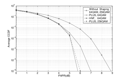
Figure 1: CCDF of PAPR for a $4\times 4$ space-time code [28] using HNF and PLUS approximate cubic shaping.

	HNF shaping	PLUS shaping
64QAM	4.9%	4.6%
256QAM		3.5%

TABLE I: Increased average power for a $4\times 4$ space-time code [28] using HNF and PLUS approximate cubic shaping.

In Fig. 2, we investigate the $5\times 5$ space-time code given in [7] which also achieves the D-MG tradeoff. Similar trends as in the $4\times 4$ case can be observed.

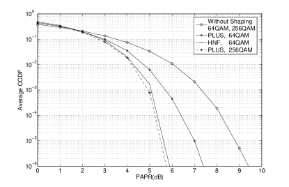
Figure 2: CCDF of PAPR for a $5\times 5$ space-time code [7] using HNF and PLUS approximate cubic shaping.

	HNF shaping	PLUS shaping
64QAM	5.4%	4.8%
256QAM		3.2%

TABLE II: Increased average power for a $5\times 5$ space-time code [7] using HNF and PLUS approximate cubic shaping.

Finally, Fig. 3 presents the codeword error probability (CEP) of systems with $4$ or $5$ receive antennas and $4$ or $5$ transmit antennas in quasi-static Rayleigh fading channels. Here, we use the perfect space-time codes in [7] and [28] for the $4\times 4$ and $5\times 5$ channels, respectively. The codeword sizes are also $4\times 4$ and $5\times 5$ symbols, respectively. The sphere decoder in [29] is used for lattice decoding. The results show that the space-time codes after shaping yield almost indistinguishable error performance compared to the performance without shaping.

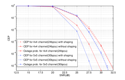
Figure 3: Codeword error probability for Rayleigh fading channel with or without shaping.

VIII Conclusion

In this paper, we first showed that, for Rayleigh fading channels, the D-MG tradeoff remains unchanged with any PAPR constraints larger than one. This result implies that, instead of designing codes on a case-by-case basis, as done by most existing works, there possibly exist general methodologies for designing space-time codes with low PAPR that achieve the optimal D-MG tradeoff. As an example of such methodologies, we proposed a PAPR reduction method based on constellation shaping that can be applied to existing optimal space-time codes without affecting their optimality in the D-MG tradeoff. Unlike most PAPR reduction methods, the proposed method does not introduce redundancy or require side information being transmitted to the decoder. Two realizations of the proposed method were considered. The first utilizes the Hermite Normal Form decomposition of integer matrices. The second utilizes the integer reversible mapping. Compared to the previous works [12][10] which applied a similar approach (Smith Normal Form) to the single-antenna OFDM systems, the proposed method has lower complexities. In addition, even though [12] managed to reduce the complexity to the same order $O(MlogM)$ as the proposed integer reversible mapping scheme (in the single-antenna OFDM case) by using a Hadamard matrix, that approach affects the PAPR reduction capability and only works for OFDM systems. The proposed method, on the other hand, works for any nonsingular generator (modulation) matrix and can achieve better PAPR reduction. Sphere decoding was performed to verify that the proposed PAPR reduction method does not affect the optimality of space-time codes.

Appendix A Proof of Lemma 1

Following the method in [20], since the receiver knows the realization of ${\bf{H}}$, the channel output is the pair $({\mathbf{y,H}})$. The mutual information between channel input and output is then

$$I\left({{\mathbf{x;(y,H)}}}\right)=I{\mathbf{(x;H)}}+I({\mathbf{x;y|H}})=I({\mathbf{x;y|H}}).$$ (44)

Denote $h(x)$ as the differential entropy of ${x}$ and let $H$ be a particular realization of ${\bf H}$. For this ${H}$, when the SNR is asymptotically large, the output differential entropy $h({\mathbf{y|H}}=H)$ can be well approximated by the input differential entropy $h({\mathbf{x|H}}=H)$. In addition,

$$I({\mathbf{x;y|H}}=H) =h({\mathbf{x|H}}=H)-h({\mathbf{x|y}},{\mathbf{H}}=H)$$ (45)

$$=h({\mathbf{x|H}}=H)-h({\mathbf{e}}|{\mathbf{y}},{\mathbf{H}}=H),$$ (46)

where $\;{\mathbf{e}}\triangleq{\mathbf{x}}-{\mathbf{F}}_{MMSE}{\mathbf{y}}$, and ${\mathbf{F}}_{MMSE}$ is the minimum mean-square error (MMSE) estimation filter of ${\bf{x}}$ given ${\bf{y}}$.

Since the lemma is to lower bound the ergodic channel capacity, any rate achieved by a particular signal can serve as a lower bound. We select the transmitted signal $\mathbf{x}$ such that $E\left[\mathbf{x}\right]=0$ and ${\mathbf{S}}_{{\mathbf{xx}}}\triangleq E\left[{{\mathbf{xx}}^{\dagger}}\right]$ is positive definite. In the following, we will compute the rate achievable by signals with these properties. This achievable rate obviously lower bounds the capacity.

Denote ${\mathbf{S}}_{{\mathbf{xy}}}\triangleq E\left[{{\mathbf{xy}}^{\dagger}}\right]$. According to the Orthogonality Principle, we have

$${\mathbf{F}}_{MMSE}\; ={\mathbf{S}}_{{\mathbf{xy}}}{\mathbf{S}}_{{\mathbf{yy}}}^{{\mathbf{-1}}}\;$$

$$={\mathbf{S}}_{{\mathbf{xx}}}H^{\dagger}{\mathbf{(}}H{\mathbf{S}}_{{\mathbf{xx}}}H^{\dagger}{\mathbf{+I)}}^{{\mathbf{-1}}}$$

$$={\mathbf{(}}H^{\dagger}H{\mathbf{+S}}_{{\mathbf{xx}}}^{{\mathbf{-1}}}{\mathbf{)}}^{{\mathbf{-1}}}H^{\dagger}$$ (47)

where the matrix inversion lemma

$${\mathbf{(A+BCD)}}^{{\mathbf{-1}}}{\mathbf{=A}}^{{\mathbf{-1}}}{\mathbf{-A}}^{{\mathbf{-1}}}{\mathbf{B(C}}^{{\mathbf{-1}}}{\mathbf{+DA}}^{{\mathbf{-1}}}{\mathbf{B)}}^{{\mathbf{-1}}}{\mathbf{DA}}^{{\mathbf{-1}}}$$

is used. $E\left[{{\mathbf{ee}}^{\dagger}}\right]$ can be computed as

$$E\left[{{\mathbf{ee}}^{\dagger}}\right] ={\mathbf{S}}_{{\mathbf{xx}}}{\mathbf{-S}}_{{\mathbf{xx}}}H^{\dagger}{\mathbf{(}}H{\mathbf{S}}_{{\mathbf{xx}}}H^{\dagger}{\mathbf{+I)}}^{{\mathbf{-1}}}H{\mathbf{S}}_{{\mathbf{xx}}}$$

$$={\mathbf{(}}H^{\dagger}H{\mathbf{+S}}_{{\mathbf{xx}}}^{{\mathbf{-1}}}{\mathbf{)}}^{{\mathbf{-1}}}$$ (48)

where the matrix inversion lemma is again used. Note that $E[{\mathbf{e}}]=0$ since $E[{\mathbf{x}}]=0$ and $E[{\mathbf{y}}]=0$. Thus the covariance matrix of ${\bf{e}}$, denoted ${\mathbf{Cov}}[{\mathbf{e}}]$, is equal to $E[{\mathbf{ee}}^{\dagger}]$. Then we have

$$\begin{split}h({\mathbf{e}}|{\mathbf{y}},{\mathbf{H}}=H)\leq h({\mathbf{e}}|{\mathbf{H}}=H)&\leq\log\det\left({\pi e{\mathbf{Cov}}[{\mathbf{e}}]}\right)\\ &=\log\det\left({\pi eE[{\mathbf{ee}}^{\dagger}]}\right)\;\end{split}.$$ (49)

Define

$$\tilde{I}({\mathbf{x;y|H}}=H) \triangleq h({\mathbf{x|H}}=H)-\log\det\left({\pi eE[{\mathbf{ee}}^{\dagger}]}\right)$$

$$=h({\mathbf{x|H}}=H)+\log\det\left({\frac{1}{{\pi e}}{\mathbf{(}}H^{\dagger}H{\mathbf{+S}}_{{\mathbf{xx}}}^{{\mathbf{-1}}}{\mathbf{)}}}\right).$$ (50)

Obviously, $\tilde{I}({\mathbf{x;y|H}}=H)\leq I({\mathbf{x;y|H}}=H)$. We have the ergodic capacity

$$\begin{gathered}C=\mathop{\max}\limits_{f_{\mathbf{x}}({\mathbf{x}})}I\left({{\mathbf{x;(y,H)}}}\right)\mathop{=}\limits^{(\ref{a9})}\mathop{\max}\limits_{f_{\mathbf{x}}({\mathbf{x}})}\;E_{\mathbf{H}}\left[{I({\mathbf{x;y|H}})}\right]\hfill\\ \;\;\;\mathop{=}\limits^{(\ref{a11})}\mathop{\max}\limits_{f_{\mathbf{x}}({\mathbf{x}})}\;E_{\mathbf{H}}\left[{h({\mathbf{x|H}})-h({\mathbf{e}}|{\mathbf{y}},{\mathbf{H}})}\right]\hfill\\ \end{gathered}$$

where $f_{\mathbf{x}}({\mathbf{x}})$ is the probability density function of ${\bf{x}}$ subject to (5) and (6). The ergodic capacity is lower bounded by

$$C =\mathop{\max}\limits_{f_{\mathbf{x}}({\mathbf{x}})}\;E_{\mathbf{H}}\left[{I({\mathbf{x;y|H}})}\right]\geq\mathop{\max}\limits_{f_{\mathbf{x}}({\mathbf{x}})}\;E_{\mathbf{H}}\left[{\tilde{I}({\mathbf{x;y|H}})}\right]$$

$$=\mathop{\max}\limits_{f_{\mathbf{x}}({\mathbf{x}})}\;E_{\mathbf{H}}\left[{h({\mathbf{x|H}})+\log\det\left({\frac{1}{{\pi e}}{\mathbf{(H}}^{\dagger}{\mathbf{H+S}}_{{\mathbf{xx}}}^{{\mathbf{-1}}}{\mathbf{)}}}\right)\;}\right]$$ (51)

$$\geq\mathop{\max}\limits_{f_{\mathbf{x}}({\mathbf{x}})}E_{\mathbf{H}}\left[{h({\mathbf{x|H}})}\right]+\left(E_{\mathbf{H}}\left[{\log\det\left({\frac{1}{{\pi e}}{\mathbf{(H}}^{\dagger}{\mathbf{H+S}}_{{\mathbf{xx}}}^{{\mathbf{-1}}}{\mathbf{)}}}\right)\;}\right]\right)_{f_{\mathbf{x}}({\mathbf{x}})=f^{*}_{\mathbf{x}}({\mathbf{x}})}$$ (52)

$$=\mathop{\max}\limits_{f_{\mathbf{x}}({\mathbf{x}})}\;h({\mathbf{x}})+\left(E_{\mathbf{H}}\left[{\log\det\left({\frac{1}{{\pi e}}{\mathbf{(H}}^{\dagger}{\mathbf{H+S}}_{{\mathbf{xx}}}^{{\mathbf{-1}}}{\mathbf{)}}}\right)}\right]\right)_{f_{\mathbf{x}}({\mathbf{x}})=f^{*}_{\mathbf{x}}({\mathbf{x}})}$$ (53)

$$\triangleq C^{\prime},$$

where $f^{*}_{\mathbf{x}}({\mathbf{x}})=\arg\mathop{\max}\limits_{f_{\mathbf{x}}({\mathbf{x}})}E_{\mathbf{H}}\left[{h({\mathbf{x|H}})}\right]=\arg\mathop{\max}\limits_{f_{\mathbf{x}}({\mathbf{x}})}\;h({\mathbf{x}})$. $f^{*}_{\mathbf{x}}({\mathbf{x}})$ and $C^{\prime}$ can be obtained by solving the following problem

$$\begin{gathered}\mathop{\max}\limits_{f_{\mathbf{x}}({\mathbf{x}})}\;h({\mathbf{x}})\\ \mbox{s.t.}\;\;\;\mbox{Tr}\left({E_{\mathbf{x}}\left[{{\mathbf{xx}}^{\dagger}}\right]}\right)\leq{\mathbf{P}}\\ \;\;\;\;\;\;\;\;\;\;\;\;\;\;\;\;\;\;\;\frac{{|x_{i}|^{2}}}{{E_{x_{i}}[|x_{i}|^{2}]}}\leq\;\rho_{i},\;\;\;i=1,\ldots,m.\end{gathered}$$ (54)

Due to the circular symmetry of the constraints (5) and (6), polar coordinates

$$\begin{gathered}{\mathbf{x}}=[x_{1},x_{2}...,x_{m}]^{T}=[r_{1}e^{j\theta_{1}},r_{2}e^{j\theta_{2}},...,r_{m}e^{j\theta_{m}}]^{T}\hfill\\ \;\;\;\;\;\;\;\;\;\;\;\;\;\;\;\;\;r_{i}\geq 0,\;\;\;\theta_{i}\in[0,2\pi)\hfill\\ \end{gathered}$$

are found convenient, where $r_{i}$ and $\theta_{i}$ stand, respectively, for the amplitude and phase of $x_{i}$. Straightforward transformation yields

$$\begin{split}h({\mathbf{x}})&=-\int{f_{\mathbf{x}}({\mathbf{x}})}\log f_{\mathbf{x}}({\mathbf{x}})d{\mathbf{x}}=-\int{f_{{\mathbf{r,\theta}}}{\mathbf{(r,\theta)}}}\log\frac{{f_{{\mathbf{r,\theta}}}{\mathbf{(r,\theta)}}}}{{\prod\limits_{i=1}^{m}{r_{i}}}}d{\mathbf{r}}d{\mathbf{\theta}}\\ &=h({\mathbf{r,\theta}})+\sum\limits_{i=1}^{m}{\left({\int{f_{r_{i}}{\mathbf{(}}r_{i}{\mathbf{)}}}\log r_{i}dr_{i}}\right)}\end{split}$$

where ${\mathbf{r}}$ and ${\mathbf{\theta}}$ are vectors consisting of $r_{i}$ and $\theta_{i}$, respectively. Note that

$$h({\mathbf{r,\theta}})\leq h({\mathbf{r}})+h({\mathbf{\theta}})\leq h({\mathbf{r}})+m\log\;2\pi.$$

Therefore, to maximize $h({\mathbf{x}})$, we should choose ${\mathbf{r}}$ and ${\mathbf{\theta}}$ independent of each other, and all $\theta_{i}$ distributed independently and uniformly in $[0,2\pi)$. Then the equality holds and

$$h({\mathbf{x}})=h({\mathbf{r}})+\sum\limits_{i=1}^{m}{\left({\int{f_{r_{i}}{\mathbf{(}}r_{i}{\mathbf{)}}}\log r_{i}dr_{i}}\right)}+m\log 2\pi.$$

Similarly,

$$h({\mathbf{r}})\leq\sum\limits_{i=1}^{m}{h(r_{i})}.$$

Choosing $r_{i}$ independent of one another, the equality holds and $h({\mathbf{x}})$ is maximized. Drop the last term of $h({\mathbf{x}})$, and transform (54) into the following equivalent optimization problem

$$\begin{gathered}\;\;\;\mathop{\max}\limits_{f_{\mathbf{r}}{\mathbf{(r)}}}\;\left({\sum\limits_{i=1}^{m}{h(r_{i})}+\sum\limits_{i=1}^{m}{\left({\int{f_{r_{i}}{\mathbf{(}}r_{i}{\mathbf{)}}}\log r_{i}dr_{i}}\right)}}\right)\hfill\\ =\mathop{\max}\limits_{f_{\mathbf{r}}{\mathbf{(r)}}}\;\left({-\sum\limits_{i=1}^{m}{\left({\int{f_{r_{i}}{\mathbf{(}}r_{i}{\mathbf{)}}}\log\frac{{f_{r_{i}}{\mathbf{(}}r_{i}{\mathbf{)}}}}{{r_{i}}}dr_{i}}\right)}}\right)\;\hfill\\ \;\;\;\;\;\;\;\;\;\;\;\;\;\;\;\;\;\;\mbox{s.t.}\;\;\;\mbox{Tr}\left({E_{\mathbf{r}}\left[{{\mathbf{rr}}^{\mathbf{*}}}\right]}\right)\leq{\mathbf{P}}\hfill\\ \;\;\;\;\;\;\;\;\;\;\;\;\;\;\;\;\;\;\;\;\;\;\;\;\;\;\;\;\;\;\;\frac{{|r_{i}|^{2}}}{{E_{r_{i}}[|r_{i}|^{2}]}}\leq\;\rho_{i},\;\;\;i=1,\ldots,m.\hfill\\ \end{gathered}$$ (55)

For each antenna $i$, given the transmission power $P_{i}$ such that

$$\sum\limits_{i=1}^{m}{P_{i}}={\mathbf{P}}$$

and a PAPR constraint $\rho_{i}$, similar to [19], the optimal solution $f_{r_{i}}^{*}(r_{i})$ is (see Appendix B)

$$\begin{split}f_{r_{i}}^{*}(r_{i})&=a_{i}r_{i}\;\exp(-b_{i}r_{i}^{2}/2),\;\;\;\;\;\forall r_{i}\in\left[{0,\sqrt{\rho_{i}P_{i}}}\right]\\ f_{r_{i}}^{*}(r_{i})&=0,\;\;\;\;\;\;\;\;\;\;\;\;\;\;\;\;\;\;\;\;\;\;\;\;\;\;\;\;\;\;\;\;\;\;\;\;\forall r_{i}\notin\left[{0,\sqrt{\rho_{i}P_{i}}}\right]\end{split}$$ (56)

where $a_{i}$, $b_{i}$ satisfy (57), (58) or (59):

$$\mbox{when}\;\;\rho_{i}\neq 2,\;\rho_{i}>1$$

$$\frac{{a_{i}}}{{b_{i}}}(1-\exp(-b_{i}\rho_{i}P_{i}/2))=1$$ (57)

$$2(a_{i}/b_{i})(b_{i}\rho_{i}P_{i})^{-1}[1-(1+b_{i}\rho_{i}P_{i}/2)\exp(-b_{i}\rho_{i}P_{i}/2)]=1/\rho_{i},$$ (58)

$$\mbox{when}{\text{ }}\rho_{i}=2$$

$$a_{i}=\frac{2}{{\rho_{i}P_{i}\;}},\;\;\;b_{i}=0.$$ (59)

Denoting the maximum of $h(x_{i})$ as $h^{*}(x_{i})$ and $c_{i}=b_{i}\rho_{i}P_{i}$, we can compute $h^{*}(x_{i})$ directly by using $f_{r_{i}}^{*}(r_{i})$

$$h^{*}(x_{i}) =-\log a_{i}+\frac{{b_{i}P_{i}}}{2}+\log 2\pi$$ (60)

$$=\;-\log a_{i}+\frac{{c_{i}}}{{2\rho_{i}}}+\log 2\pi$$ (61)

$$=\left.\begin{cases}\log P_{i}+\log\frac{{\rho_{i}(1-\exp(-c_{i}/2))}}{{c_{i}}}+\frac{{c_{i}}}{{2\rho_{i}}}+\log 2\pi,\;\;\;\;\;\;&\rho_{i}\neq 2,~{}\rho_{i}>1\\ \log{{2\pi}{P_{i}}},&\rho_{i}=2\end{cases}\right..$$ (62)

From (57), $(1-\exp(-b_{i}\rho_{i}P_{i}/2))^{-1}=\frac{{a_{i}}}{{b_{i}}}$. By substituting $\frac{{a_{i}}}{{b_{i}}}$ in (58) with $(1-\exp(-b_{i}\rho_{i}P_{i}/2))^{-1}$ and then replacing $b_{i}\rho_{i}P_{i}$ with $c_{i}$, we will arrive at

$$\frac{2}{c_{i}}-\frac{1}{1-\exp(-c_{i}/2)}+1=\frac{1}{\rho_{i}}$$

which indicates that $1/\rho_{i}$ is a monotonic function of $c_{i}$, as shown in Fig. 4. Thus, when $\rho_{i}>1$ is fixed and finite, $c_{i}$ is a finite constant. With the independence between $x_{i}$’s,

$$h^{*}({\mathbf{x}})=\sum\limits_{i=1}^{m}{h^{*}(x_{i})}.$$

Now we can plug $h^{*}({\mathbf{x}})$ and the corresponding (independent) distribution of ${\mathbf{x}}$ into (53) to obtain the lower bound $C^{\prime}$ of the ergodic capacity. Let

$$k_{i}=\begin{cases}\log\frac{{\rho_{i}(1-\exp(-c_{i}/2))}}{{c_{i}}}+\frac{{c_{i}}}{{2\rho_{i}}}+\log\frac{2}{e},\;\;\;\;\;\;&\rho_{i}\neq 2,~{}\rho_{i}>1\\ \log\frac{2}{e},&\rho_{i}=2\end{cases}$$

which is a constant because $c_{i}$ is a finite constant when $\rho_{i}>1$ is fixed and finite. We have

$$C^{\prime}=E_{\mathbf{H}}\left[{\log\det\left({{\mathbf{I}}+{\mathbf{H}}{\mathbf{S}}_{{\mathbf{xx}}}{\mathbf{H}}^{\dagger}}\right)}\right]+\sum\limits_{i=1}^{m}{k_{i}},$$

where the equality follows from the determinant identity $\det({\mathbf{I+AB}})=\det({\mathbf{I+BA}})$. With the selection of equal-power allocation, $P_{i}={\mathbf{P}}/m$, $\forall i$. Thus

$$C\geq C^{\prime}=E_{\mathbf{H}}\left[{\log\det\left({{\mathbf{I}}+\frac{{\mathbf{P}}}{m}{\mathbf{H}}{\mathbf{H}}^{\dagger}}\right)}\right]+\sum\limits_{i=1}^{m}{k_{i}}.$$ (63)

Note that the inequality holds for any distribution of $\mathbf{H}$. When $\rho_{i}\to\infty$, $a_{i}=b_{i}=2/P_{i}$, and

$$C=C^{\prime}=E_{\mathbf{H}}\left[{\log\det\left({{\mathbf{I}}+\frac{{\mathbf{P}}}{m}{\mathbf{H}}{\mathbf{H}}^{\dagger}}\right)}\right]$$

which is the classical result without PAPR constraints. The constant $k_{i}$ (i.e., the difference between $h^{*}(x_{i})$ when $\rho_{i}\to\infty$ and when $\rho_{i}$ is finite) is shown in Fig. 5.

Appendix B Derivation of the Optimal Signal Probability Density Functions

We consider the following optimization problem with average power and PAPR constraints

$$\begin{gathered}\;\;\mathop{\max}\limits_{f_{r}{\mathbf{(}}r{\mathbf{)}}}\;\left({-\int{f_{r}{\mathbf{(}}r{\mathbf{)}}}\log\frac{{f_{r}{\mathbf{(}}r{\mathbf{)}}}}{r}dr}\right)\;\hfill\\ \;\;\;\;\mbox{s.t.}\;\;\;\;\;E\left[{|r|^{2}}\right]\leq P\hfill\\ \;\;\;\;\;\;\;\;\;\;\;\;\;\;\frac{{|r|^{2}}}{{E[|r|^{2}]}}\leq\;\rho.\;\;\;\;\hfill\\ \end{gathered}$$ (64)

Note that the PAPR constraint is different from the peak power constraint considered in [19], thus the results in [19] do not directly apply to our case. The following derivation (verification) is necessary. The problem will be solved through the following slightly different problem with average and peak power constraints

$$\begin{gathered}\;\;\;\mathop{\max}\limits_{f_{r}{\mathbf{(}}r{\mathbf{)}}}\;\left({-\int{f_{r}{\mathbf{(}}r{\mathbf{)}}}\log\frac{{f_{r}{\mathbf{(}}r{\mathbf{)}}}}{r}dr}\right)\;\hfill\\ \;\;\;\;\mbox{s.t.}\;\;\;\;\;E\left[{|r|^{2}}\right]\leq P\hfill\\ \;\;\;\;\;\;\;\;\;\;\;\;\;\;\;\;\;\;\;\;\;|r|^{2}\leq\;\rho P\;\hfill\\ \end{gathered}$$ (65)

which can be rewritten as

$$\begin{gathered}\mathop{\max}\limits_{f_{r}{\mathbf{(}}r{\mathbf{)}}}-\left({\int_{0}^{\sqrt{\rho P}}{f_{r}(r)\log\frac{{f_{r}(r)}}{r}dr}}\right)\hfill\\ \;\mbox{s.t.}\;\;\;\;\;f_{r}(r)\geq 0,\;\;\;\;\forall r\in[0,\sqrt{\rho P}]\hfill\\ \;\;\;\;\;\;\;\;\;\;\int_{0}^{\sqrt{\rho P}}{f_{r}(r)dr=1}\hfill\\ \;\;\;\;\;\;\;\;\;\int_{0}^{\sqrt{\rho P}}{r^{2}f_{r}(r)dr\leq P}.\;\;\hfill\\ \end{gathered}$$ (66)

The optimal solution $f_{r}^{*}(r)$ of (66) is given by the standard variational techniques [19]

$$f_{r}^{*}(r) =ar{}\exp(-br^{2}/2),\;\;\;\;\;\;\;\;\ \forall r\in\left[{0,\sqrt{\rho P}}\right]$$ (67)

$$f_{r}^{*}(r) =\;\;\;\;0,\;\;\;\;\;\;\;\;\;\;\;\;\;\;\;\;\;\;\;\;\;\;\;\;\;\;\;\;\;\;\;\;\forall r\neq\left[{0,\sqrt{\rho P}}\right].$$ (68)

Observe that if the first equality in (65) holds, the optimal solution $f_{r}^{*}(r)$ of (66) is also the optimal solution of (64). However, the equality does not always hold.

We discuss $a$, $b$ for different values of PAPR ($\rho>1$). When $\rho>2$, $a$, $b$ satisfy

$$\frac{a}{b}(1-\exp(-b\rho P/2))=1$$ (69)

$$2(a/b)(b\rho P)^{-1}[1-(1+b\rho P/2)\exp(-b\rho P/2)]=1/\rho.\;$$ (70)

Equations (69) and (70) together solve $b$ as a function of $\rho$ and $P$ which is illustrated in Fig. 4 with $T=\rho P/2$. Fig. 4 shows that $b>0$ when $\rho>2$. Thus the first equality in (65) holds and $f_{r}^{*}(r)$ is also the optimal solution of (64). Note that when $\rho\to\infty$, $a=b=2/P$ and $f_{r}^{*}(r)$ is the Rayleigh distribution as expected.

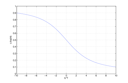
Figure 4: The relation between $bT$ ($bT=b\rho P/2=c/2$, as defined in Appendix A, before (60)) and $1/\rho$ subject to (69) and (70).

When $\rho=2$, $a$, $b$ satisfy

$$b=0,\;\;a=1/P.$$ (71)

In this case, $f_{r}^{*}(r)$ is linear and the equality in (65) is again satisfied and $f_{r}^{*}(r)$ is the optimal solution of (64).

For the case of $\rho<2$, the Karush-Kuhn-Tucker (KKT) conditions for the optimization problem (66) require that $b\geq 0$. However, from Fig. 4, $b<0$ when $\rho<2$. Therefore, $a$, $b$ for the optimal solution of (66) should satisfy (71). In this situation

$$\int_{0}^{\sqrt{\rho P}}{r^{2}f_{r}^{*}(r)dr=\frac{\rho}{2}P<P}.$$ (72)

That is, the first equality in (65) does not hold, and the corresponding PAPR value is $2$, larger than $\rho$. As a result, $f_{r}^{*}(r)$ is not the optimal solution of (64).

To obtain the optimal solution of (64) when $\rho<2$, consider the following problem with slightly different constraints

$$\begin{gathered}\;\;\mathop{\max}\limits_{f_{r}{\mathbf{(}}r{\mathbf{)}}}\;\left({-\int{f_{r}{\mathbf{(}}r{\mathbf{)}}}\log\frac{{f_{r}{\mathbf{(}}r{\mathbf{)}}}}{r}dr}\right)\;\hfill\\ \;\;\;\;\mbox{s.t.}\;\;\;\;\;E\left[{|r|^{2}}\right]=P\hfill\\ \;\;\;\;\;\;\;\;\;\;\;\;\;\;\;\;\;\;\;\;\;|r|^{2}\leq\;\rho P.\;\hfill\\ \end{gathered}$$ (73)

Using similar optimization techniques, the optimal solution of (73), $f_{r}^{\prime}(r)$, is found to have the same form as (67), (68) with $b<0$. Therefore, $f_{r}^{\prime}(r)$ is not a Rayleigh-like distribution. We will show that $f_{r}^{\prime}(r)$ is also the optimal solution of (64). Assuming that the distribution $f_{r}^{\prime\prime}(r)$ is the optimal solution of (64) and $f_{r}^{\prime\prime}(r)\neq f_{r}^{\prime}(r)$, then $f_{r}^{\prime\prime}(r)$ must be the optimal solution of the following optimization problem for some $P^{\prime\prime}$

$$\begin{gathered}\;\mathop{\max}\limits_{f_{r}{\mathbf{(}}r{\mathbf{)}}}\;\left({-\int{f_{r}{\mathbf{(}}r{\mathbf{)}}}\log\frac{{f_{r}{\mathbf{(}}r{\mathbf{)}}}}{r}dr}\right)\;\hfill\\ \;\;\;\;\mbox{s.t.}\;\;\;\;\;E\left[{|r|^{2}}\right]=P^{\prime\prime}<P\hfill\\ \;\;\;\;\;\;\;\;\;\;\;\;\;\;\;\;\;|r|^{2}\leq\;\rho P^{\prime\prime}<\rho P.\;\;\hfill\\ \end{gathered}$$ (74)

However, (73) has a larger maximum value, namely $(-\log a+bP/2)$, than that of (74) because $P>P^{\prime\prime}$, which implies that $f_{r}^{\prime}(r)$ maximizes (64). In Fig. 5, we demonstrate the maximum values of $h^{*}(x)$, where $h^{*}(x)=(-\log a+bP/2+\log 2\pi)$, for $\rho=5,\;\;2,\;\;1.1,\;\;\infty$.

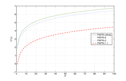
Figure 5: The maximum value $h^{*}(x)$ for different $\rho$ (PAPR) values

Appendix C Proof of Theorem 2

We follow the method in [1], letting the $i$-th element of the input signal be drawn from the random code with i.i.d. distribution $f_{x_{i}}^{*}(x_{i})$

$$\begin{split}f_{x_{i}}^{*}(x_{i})&=\frac{1}{2\pi}a_{i}exp\left(-\frac{b_{i}}{2}|x_{i}|^{2}\right),\;\;\;\;x_{i}\in\textbf{B}_{i}\\ f_{x_{i}}^{*}(x_{i})&=0,\;\;\;\;\;\;\;\;\;\;\;\;\;\;\;\;\;\;\;\;\;\;\;\;\;\;\;\;\;\;\;\,\;\;\;\;\;\;\;\;\;x_{i}\notin\textbf{B}_{i}\end{split}$$ (75)

where $x_{i}\in\mathbb{C}$, $\textbf{B}_{i}\triangleq\{x_{i}\mathbf{\mid}\;\;|x_{i}|\leq\sqrt{\rho_{i}P_{i}}\;\}$. At data rate $R=rlogSNR$, the error probability is

$$P_{e}(SNR)\leq P_{out}(R)+P(error,no\;outage).$$

The second term can be upper bounded via a union bound. Assume that $X(0)$, $X(1)$ are two possible transmitted codewords, and ${\Delta X}={X(1)-X(0)}$. Suppose that $X(0)$ is transmitted. The probability that a maximum likelihood receiver will make a detection error in favor of $X(1)$, conditioned on a certain realization of the channel, is

$$P\left({X(0)\to X(1)|{\mathbf{H}}=H}\right) =P\left({\left\|{\frac{1}{2}H{\Delta X}}\right\|^{2}\leq\left\|{\mathbf{w}}\right\|^{2}}\right)$$ (76)

$$\leq exp\left[-\frac{1}{4}\|H\Delta X\|^{2}\right]$$ (77)

where $\mathbf{w}$ is the additive noise on the direction of $H\Delta X$. Then we need to average over the ensemble of random codes. Let $x_{i}$ and $x^{\prime}_{i}$ be two i.i.d. random variables with distribution in the form of (75), and $x^{\prime}_{i}-x_{i}=\hat{x}_{i}$. The probability density function of $\hat{x}_{i}$ is

$$\begin{split}f_{\hat{x_{i}}}(\hat{x_{i}})=\frac{1}{2\pi}a_{i}{}exp\left(-\frac{b_{i}}{4}|\hat{x_{i}}|^{2}\right)\int_{x_{i}\in\mathbf{C}_{i}}\frac{1}{2\pi}a_{i}{}exp\left(-b_{i}|x_{i}-\frac{\hat{x_{i}}}{2}|^{2}\right)dx_{i}\end{split}$$ (78)

where $x_{i}\in\mathbf{C}_{i}$ if $\;\;x_{i}\in\textbf{B}_{i}$ and $x^{\prime}_{i}\in\textbf{B}_{i}$. We discuss different values of $b_{i}$.

For $b_{i}>0$,

$$\int_{x_{i}\in\mathbf{C}_{i}}\frac{1}{2\pi}a_{i}{}exp\left(-b_{i}|x_{i}-\frac{\hat{x_{i}}}{2}|^{2}\right)dx_{i}\leq\int_{x_{i}\in\mathbb{C}}\frac{1}{2\pi}a_{i}{}exp\left(-b_{i}|x_{i}-\frac{\hat{x_{i}}}{2}|^{2}\right)dx_{i}=t_{1}$$ (79)

where $t_{1}$ is a constant, which is independent of of $P_{i}$.

For $b_{i}=0$, since $|x_{i}-\frac{\hat{x_{i}}}{2}|\leq 2\sqrt{\rho_{i}P_{i}}$ and $a_{i}P_{i}{\rho_{i}}=\rho_{i}$

$$\int_{x_{i}\in\mathbf{C}_{i}}\frac{1}{2\pi}a_{i}{}exp\left(-b_{i}|x_{i}-\frac{\hat{x_{i}}}{2}|^{2}\right)dx_{i}\leq\int_{x_{i}\in\mathbb{C}}\frac{1}{2\pi}a_{i}{}exp\left(-a_{i}|x_{i}-\frac{\hat{x_{i}}}{2}|^{2}\right)exp\left(4a_{i}\rho_{i}{P_{i}}\right)dx_{i}=t_{2}$$ (80)

where $t_{2}$ is a constant, which is independent of of $P_{i}$.

For $b_{i}<0$, since $|x_{i}-\frac{\hat{x_{i}}}{2}|\leq 2\sqrt{\rho_{i}{P_{i}}}$ and $b_{i}P_{i}{\rho_{i}}$ is a constant.

$$\int_{x_{i}\in\mathbf{C}_{i}}\frac{1}{2\pi}a_{i}{}exp\left(-b_{i}|x_{i}-\frac{\hat{x_{i}}}{2}|^{2}\right)dx_{i}\leq\int_{x_{i}\in\mathbb{C}}\frac{1}{2\pi}a_{i}{}exp\left(b_{i}|x_{i}-\frac{\hat{x_{i}}}{2}|^{2}\right)exp\left(-8b_{i}\rho_{i}{P_{i}}\right)dx_{i}=t_{3}$$ (81)

where $t_{3}$ is a constant, which is independent of of $P_{i}$.

Thus we have

$$f_{\hat{x_{i}}}(\hat{x_{i}}) \leq c_{i}\cdot\frac{1}{2\pi}a_{i}{}exp\left(-\frac{b_{i}}{4}|\hat{x_{i}}|^{2}\right)$$ (82)

$$\leq d_{i}c_{i}\cdot\frac{1}{2\pi}a_{i}{}exp\left(-\frac{b^{\prime}_{i}}{4}|\hat{x_{i}}|^{2}\right)$$ (83)

$$\leq d_{i}c_{i}\cdot\frac{1}{2\pi}a_{i}{}exp\left(-\frac{b_{min}}{4}|\hat{x_{i}}|^{2}\right)$$ (84)

where $c_{i}=t_{1}$, $t_{2}$, or $t_{3}$. (83) follows from (82) by using the same techniques as above and $d_{i}$ is a constant independent of $P_{i}$. $b_{min}=\min(b^{\prime}_{i})$, where $b^{\prime}_{i}=b_{i}$ for $b_{i}>0$; $b^{\prime}_{i}=a_{i}$ for $b_{i}=0$; $b^{\prime}_{i}=-b_{i}$ for $b_{i}<0$. The average pairwise error probability given the channel realization is

$$\overline{P}\left(X(i)\to X(j),i\neq j|{\mathbf{H}}=H\right)\leq\tilde{K}\left({\prod\limits_{i=1}^{m}{a_{i}}}\right)^{l}\det\left({{b_{min}I}+HH^{\dagger}}\right)^{-l}$$ (85)

where $\tilde{K}$ is a constant which is not important here. At a data rate $R=r\log{SNR}$, we have a total of ${SNR}^{lr}$ codewords. Applying the union bound, we have

$$P\left({error|{\mathbf{H}}=H}\right)\leq \tilde{K}{SNR}^{lr}\left({\prod\limits_{i=1}^{m}{a_{i}}}\right)^{l}\det\left({{b_{min}I}+HH^{\dagger}}\right)^{-l}$$

$$= \tilde{K}{SNR}^{lr}\left({\prod\limits_{i=1}^{m}\frac{a_{i}}{b_{\min}}}\right)^{l}\det\left({I+\frac{1}{b_{\min}}HH^{\dagger}}\right)^{-l}$$

$${\dot{\leq}} \tilde{K}^{\prime}{SNR}^{lr}\det\left({I+{SNR}HH^{\dagger}}\right)^{-l}$$

$$= \tilde{K}^{\prime}{SNR}^{lr}\prod\limits_{i=1}^{\min(m,n)}{\left({1+{SNR}\lambda_{i}}\right)^{-l}}$$

$$\doteq {SNR}^{-l\left[{\sum\nolimits_{i=1}^{\min(m,n)}{\left({1-\alpha_{i}}\right)^{+}-r}}\right]}$$ (86)

where $\lambda_{i}$ are the singular values of $H$ and $\lambda_{i}={SNR}^{-\alpha_{i}}$. Equation (86) is exactly the same as (19) of [1]. Following the remaining steps in [1], it can be shown that for $l\geq(m+n-1)$, the D-MG tradeoff with PAPR constraints is achievable.

References

- [1] L. Zheng and D. N. C. Tse, “Diversity and multiplexing: A fundamental tradeoff in multiple antenna channels,” IEEE Trans. Inf. Theory, vol. 49, no. 5, pp. 1073–1096, May. 2003.
- [2] H. Yao and G. W. Wornell, “Achieving the full mimo diversity-multiplexing frontier with rotation based space-time codes,” in Allerton Conf. Comm. Control and Computing., Oct 2003.
- [3] P. Dayal and M. K. Varanasi, “An optimal two transmit antenna spacetime code and its stacked extension,” in Asilomar Conf. on Signals, Systems and Computers, Monterey, CA, Nov 2003.
- [4] S. Tavildar and P. Viswanath, “Approximately universal codes over slow fading channels,” Submitted to IEEE Trans. Inform. Theory, Feb 2005.
- [5] J.-C. Belfiore, G. Rekaya, and E.Viterbo, “The golden code: a full-rate space-time code with non-vanishing determinants,” IEEE Trans. Inf. Theory, vol. 51, no. 4, pp. 1432–1436, April 2005.
- [6] H. E. Gamal, G. Caire, and M. Damen, “Lattice coding and decoding achieve the optimal diversity-multilpexing tradeoff of mimo channels,” IEEE Trans. Inf. Theory, vol. 50, pp. 968–985, June 2004.
- [7] P. Elia, B. Sethuraman, and P. V. Kumar, “Perfect space time codes with minimum and non-minimum delay for any number of antennas,” preprint, submited to arXiv:cs.IT, Dec 2005.
- [8] P. Elia, S. A. Pawar, K. R. Kumar, P. V. Kumar, and H. Lu, “Explicit space-time codes achieving the diversity-multiplexing gain tradeoff,” IEEE Trans. Inf. Theory, vol. 52, no. 9, Sep 2006.
- [9] P. Dayal and M. K. Varanasi, “Maximal diversity algebraic space-time codes with low peak-to-mean power ratio,” IEEE Trans. Inf. Theory, vol. 51, pp. 1961–1708, May 2005.
- [10] H. Kwok, “Shape up: peak-power reduction via constellation shaping,” Ph.D. dissertation, University of Illinois at Urbana-Champaign, 2001.
- [11] H. J. Smith, “On systems of linear indeterminate equations and congruences,” Philos. Trans. R. Soc. Lond., vol. 151, pp. 293–326, June 1861.
- [12] A. Mobasher and A. K. Khandani., “Integer-based constellation shaping method for papr reduction in ofdm systems,” IEEE Trans. Commun., vol. 54, pp. 119–127, Jan 2006.
- [13] C. Hermite, “Sur l introduction des variables continues dans la theorie des nombres,” J. Reine Angew. Math., pp. 191–216, 1851.
- [14] A. Storjohann, “Computation of hermite and smith normal forms of matrices,” Master’s thesis, University of Waterloo, Canada, 1994.
- [15] P. Hao and Q. Shi, “Matrix factorizations for reversible integer mapping,” IEEE Trans. Signal Process., vol. 49, pp. 2314–2324, Oct 2001.
- [16] P. Hao, “Customizable triangular factorizations of matrices,” Linear Algebra and Its Applications, vol. 382, pp. 135–154, May 2004.
- [17] H. G. Myung, J. Lim, and D. J. Goodman, “Single carrier FDMA for uplink wireless transmission,” IEEEE Vehicular Technology Magazine, vol. 1, pp. 30–38, Sept. 2006.
- [18] J. G. Smith, “On the information capacity of peak and average power constrained gaussian channels,” Ph.D. dissertation, Univ. of California, Berkeley, CA, 1969.
- [19] S. Shamai and I. Bar-David, “The capacity of average and peak powerlimited quadrature gaussian channels,” IEEE Trans. Inf. Theory, vol. 41, no. 4, pp. 060–1071, 1995.
- [20] I. E. Telatar, “Capacity of multi-antenna gaussian channels,” Tech. Rep:Bell Labs, Lucent Technologies, 1995.
- [21] G. J. Foschini, “Layered space-time architecture for wireless communication in a fading environment when using multi-element antennas,” Bell Labs Tech., vol. 1, no. 2, pp. 41–59, 1996.
- [22] G. D. Forney Jr. and L.-F. Wei, “Multidimensional constellations I: Introduction, figures of merit, and generalized cross constellations,” IEEE J. Sel. Areas Commun., pp. 877–892, Aug 1989.
- [23] G. D.Forney, “Trellis shaping,” IEEE Trans. Inf. Theory, vol. 38, pp. 281–300, Mar 1992.
- [24] A. K. Khandani and P. Kabal, “Shaping multidimensional signal spaces- part I: Optimum shaping, shell mapping,” IEEE Trans. Inf. Theory, pp. 1794–1808, Nov 1993.
- [25] R. Laroia, N. Favardin, and S. Tretter, “On optimal shaping of multidimensional constellations,” IEEE Trans. Inf. Theory, June 1994.
- [26] S. Oraintara, Y.-J.Chen, and T. Q.Nguyen, “Integer fast fourier transform,” IEEE Trans. Signal Process., vol. 50, pp. 607–618, Mar 2002.
- [27] F. A. M. L.Bruckens and A. W. M. van den Enden, “New networks for perfect inversion and perfect reconstruction,” IEEE J. Sel. Areas Commun., vol. 10, 1992.
- [28] F. Oggier, G. Rekaya, J.-C. Belfiore, and E. Viterbo, “Perfect space-time block codes,” Submitted to IEEE Trans. Inform. Theory, 2006.
- [29] A. Murugan, H. El Gamal, M. Damen, and G. Caire, “A unified framework for tree search : Rediscovering the sequential decoder,” IEEE Trans. Inf. Theory, vol. 52, no. 3, pp. 933–953, Mar. 2006.