Exhaustive Generation of Orthomodular Lattices with Exactly One Non-Quantum State

Abstract

We propose a kind of reverse Kochen-Specker theorem that amounts to generating orthomodular lattices (OMLs) with exactly one state that do not admit properties of the Hilbert space. We apply MMP algorithms to obtain smallest OMLs with 35 atoms and 35 blocks (35-35) and all other ones up to 38-38. We find out that all but one of them admit exactly one state and discover several other properties of theirs. Previously known such OMLs have 44 atoms and 44 blocks or more. We present some of them in our notation.

url]http://m3k.grad.hr/pavicic

1 Introduction

If we assumed that values of measured observables of a quantum system in all possible setups were completely independent of and unaffected by measurements of other observables of the same system, then—according to the Kochen-Specker theorem—we would run into a contradiction for particular setups.

Such setups that cannot be given a classical interpretation were not easy to find and only a handful of them have been found until 2004 by Simon Kochen and E. P. Specker [1], Asher Peres [2], Jason Zimba and Roger Penrose [3], Adán Cabello [4], Michael Kernaghan [5], and others [6, 7, 8, 9, 10]. In 2004 we designed an algorithm and wrote programs for exhaustive generation of Kochen-Specker (KS) setups by means of MMP diagrams (hypergraphs), state evaluation, and interval analysis. [11, 12]

In a 3-dim space there is a correspondence between the MMP diagrams applied to a generation of orthogonal vectors from the Hilbert space and the Greechie diagrams of orthomodular lattices (OMLs) underlying the space. The correspondence stems from the fact that a 3-dim system of equations representing orthogonalities as defined in a KS setup can have real solutions only for loops of order five and bigger and that means that MMP diagrams can be interpreted as Greechie diagrams of OMLs. [12] (Greechie diagrams with a loop of order less then five do not represent a lattice.) Hence, when we want to find KS vectors we first find OMLs that do not admit a classically strong set of states (Def. 2.3) of type 0-1 and only then we look whether there are underlying vectors according to the procedure given in  [12].

This result also enables us to take the opposite approach and find OMLs that do not admit a strong set of states at all (Def. 2.3). Since any Hilbert space admits a strong set of states this means that such OMLs cannot underly any Hilbert space and that there cannot exist “quantum states” defined on such OMLs in the same sense in which there cannot exist 0-1 (“classical”) states on KS OMLs. Thus we can view our generation of OMLs that do not admit a strong set of states as a kind of reverse Kochen-Specker theorem. Of course, since no strong set of states is admitted there can be no vectors underlying these OMLs and they cannot be used for proving the Kochen-Specker theorem.

Nevertheless the project turns out to be equally complicated as the aforementioned exhaustive generation of OMLs that do not admit 0-1 for the aforementioned Kochen-Specker setups but fortunately our previous results help. [13, 14, 12]

Our approach is based on generating and recognising orthomodular lattices that do not admit any of the properties of Hilbert lattices underlying Hilbert space. So no set of experimental detections along directions determined by such orthomodular lattices could be consistent with any quantum measurement. Note here that we cannot have a simple inversion, i.e., we cannot have classical measurement that would not be quantum because the distributivity is a stronger property than orthomodularity or modularity and non-orthomodularity immediately means non-distributivity as well. We can carry out a classical algorithm on a quantum computer but not the other way round.

In this paper we investigate one of possible realisations of the approach—orthomodular lattices with “exactly one state,” reviewed in 2008 by Mirko Navara [16] and also called nearly exotic [17]. Orthomodular lattices with exactly one state were considered by Frederic W. Shultz [18], Pavel Pták [17], Mirko Navara [19], Hans Weber [20], and others [21, 22]. They proved useful in obtaining many new properties of orthomodular lattices and other algebras.

We realized that orthomodular lattices with exactly one state are examples of our “non-quantum” lattices after we proved that their single states cannot belong to a strong set of states. We then noticed that apparently no one of the authors pointed out that their orthomodular lattices with exactly one state do not admit a strong set of states and apparently also not any stronger condition than the orthomodularity itself and we considered that worth checking.

Our approach in the present paper is to apply our algorithm for exhaustive generation of arbitrary 3D MMP diagrams to obtain orthomodular lattices with exactly one state. As an example we generate the smallest Greechie diagrams of the kind with 35-35 atoms/blocks (vertices/edges) to 38-38 atoms/blocks, present some of them graphically and discuss their properties. We also announce a new generation of algorithms and programs that will be specially designed for obtaining such lattices for arbitrary high number of atoms/blocks theoretically and much higher number of them realistically.

2 Orthomodular Lattices, MMP Diagrams, and States

Closed subspaces of the Hilbert space form an algebra called a Hilbert lattice. A Hilbert lattice is a kind of orthomodular lattice. In any Hilbert lattice the operation meet, $a\cap b$, corresponds to set intersection, ${\cal H}_{a}\bigcap{\cal H}_{b}$, of subspaces ${\cal H}_{a},{\cal H}_{b}$ of Hilbert space ${\cal H}$, the ordering relation $a\leq b$ corresponds to ${\cal H}_{a}\subseteq{\cal H}_{b}$, the operation join, $a\cup b$, corresponds to the smallest closed subspace of $\cal H$ containing ${\cal H}_{a}\bigcup{\cal H}_{b}$, and the orthocomplement $a^{\prime}$ corresponds to ${\cal H}_{a}^{\perp}$, the set of vectors orthogonal to all vectors in ${\cal H}_{a}$. Within Hilbert space there is also an operation which has no a parallel in the Hilbert lattice: the sum of two subspaces ${\cal H}_{a}+{\cal H}_{b}$ which is defined as the set of sums of vectors from ${\cal H}_{a}$ and ${\cal H}_{b}$. We also have ${\cal H}_{a}+{\cal H}_{a}^{\perp}={\cal H}$.

One can define all the lattice operations on Hilbert space itself following the above definitions (${\cal H}_{a}\cap{\cal H}_{b}={\cal H}_{a}\bigcap{\cal H}_{b}$, etc.). Thus we have ${\cal H}_{a}\cup{\cal H}_{b}=\overline{{\cal H}_{a}+{\cal H}_{b}}=({\cal H}_{a}+{\cal H}_{b})^{\perp\perp}=({\cal H}_{a}^{\perp}\bigcap{\cal H}_{b}^{\perp})^{\perp}$, [23, p. 175] where $\overline{{\cal H}_{c}}$ is the closure of ${\cal H}_{c}$, and therefore ${\cal H}_{a}+{\cal H}_{b}\subseteq{\cal H}_{a}\cup{\cal H}_{b}$. When ${\cal H}$ is finite dimensional or when the closed subspaces ${\cal H}_{a}$ and ${\cal H}_{b}$ are orthogonal to each other then ${\cal H}_{a}+{\cal H}_{b}={\cal H}_{a}\cup{\cal H}_{b}$. [24, pp. 21-29], [25, pp. 66,67], [26, pp. 8-16] Every Hilbert space is orthomodular: ${\cal H}_{a}\equiv{\cal H}_{b}\ {\buildrel\rm def\over{=}}\ ({\cal H}_{a}\cap{\cal H}_{b})\cup({\cal H}_{a}^{\perp}\cap{\cal H}_{b}^{\perp})={\cal H}\quad\Longrightarrow\quad{\cal H}_{a}={\cal H}_{b}$.

Formalising the above operations we can define orthomodular lattice as follows:

Definition 2.1.

An orthomodular lattice (OML) is an algebra $\langle{\mathcal{L}}_{0},^{\prime},\cup,\cap\rangle$ such that the following conditions are satisfied for any $a,b,c\in\,{\mathcal{L}}_{0}$ [27, L1-L6 & L7$\,{}^{\prime}$(Th. 3.2)]:

$$a\cup b\>=\>b\cup a$$ (1)

$$(a\cup b)\cup c\>=\>a\cup(b\cup c)$$ (2)

$$a^{\prime\prime}\>=\>a$$ (3)

$$a\cup(b\cup b\,^{\prime})\>=\>b\cup b\,^{\prime}$$ (4)

$$a\cup(a\cap b)\>=\>a$$ (5)

$$a\cap b\>=\>(a^{\prime}\cup b\,^{\prime})^{\prime}$$ (6)

$$a\equiv b=1\quad\Longrightarrow\quad a=b,$$ (7)

where $a\equiv b\ {\buildrel\rm def\over{=}}\ (a\cap b)\cup(a^{\prime}\cap b^{\prime})$. In addition, since $a\cup a^{\prime}=b\cup b\,^{\prime}$ for any $a,b\in\,{\mathcal{L}}_{0}$, we define the greatest element of the lattice (1) and the least element of the lattice (0):

$$\qquad\textstyle{1}\,{\buildrel\rm def\over{=}}a\cup a^{\prime},\qquad\qquad\rm\textstyle{0}\,{\buildrel\rm def\over{=}}a\cap a^{\prime}$$ (8)

the ordering relation ($\leq$) on the lattice:

$$\qquad a\leq b\ \quad{\buildrel\rm def\over{\Longleftrightarrow}}\quad\ a\cap b=a\quad\Longleftrightarrow\quad a\cup b=b$$ (9)

and the orthogonality

$$a\perp b\ \quad{\buildrel\rm def\over{\Longleftrightarrow}}\quad\ a\leq b^{\prime}.$$ (10)

Now let us look at the orthogonal vectors that determine directions in which we can orient our detection devices and therefore also directions of observable projections. We can choose one-dimensional subspaces ${\cal H}_{a},\dots,{\cal H}_{e}$ as shown in Fig. 1, where we denote them as $a,\dots,e$.

Figure 1: MMP/Greechie diagram, and its corresponding Hasse diagram.

If we used Greechie diagrams for the purpose, we would obtain the following structure of Hasse diagrams for OMLs of one dimensional Hilbert subspaces. The given orthogonalities are $a\perp b,c,d,e$ since $a\leq b^{\prime},c^{\prime},d^{\prime},e^{\prime}$, $b\perp c$ since $b\leq c^{\prime}$, and $d\perp e$ since $d\leq e^{\prime}$. Also, e.g., $b^{\prime}$ is the complement of $b$ and that means a plane to which $b$ is orthogonal: $b^{\prime}=a\cup c$. Eventually $b\cup b^{\prime}=1$ where $1$ stands for $\cal H$. However, we should better use MMP diagrams for which the bare orthogonalities between vectors suffice without the exponentially increasing complexity of Hasse diagrams.

Thus we generate orthomodular lattices as Hilbert vectors with the help of MMP diagrams that are defined by means of the following MMP algorithm [11, 12] (see a graphical representation in [12]):

• Every vertex (atom) belongs to at least one edge (block);

• Every edge contains at least 3 vertices;

• Edges that intersect each other in $n-2$ vertices contain at least $n$ vertices.

As opposed to Greechie diagrams, MMP ones are bare hypergraphs—set of vertices and edges with no other meaning or conditions imposed on them. Greechie diagrams are by definition a shorthand notation for Hasse diagrams; e.g., they have a built-in condition that they cannot contain loops of order (3) 4 or less for describing (partially ordered sets) lattices. MMP diagrams do not have any such qlimitation. For example, to obtain Kochen-Specker vectors we used 4D MMP diagrams with loops of order 2.

However, we always build additional conditions into the generation algorithm depending on application. For instance, while generating 3D OMLs or 3D Hilbert vectors we built in the orthogonality conditions—by means of a preliminary pass. In 3D they have the same effect as the condition of not having loops of order 4 or less but are much more efficient and speed up the programs tremendously. The 3D MMP diagrams we obtain in the next section are also

Greechie diagrams because 3D MMP diagrams applied to generation of either Hilbert vectors or OMLs are isomorphic (at the level of vertices and edges) to correlated Greechie diagrams.

We now ascribe a state (a value) to each lattice element in the following standard and well-known way.

Definition 2.2.

A state on an orthomodular lattice OML is a function $m:{\rm OML}\longrightarrow[0,1]$ (for real interval $[0,1]$) such that $m(1)=1$ and $a\perp b\ \Rightarrow\ m(a\cup b)=m(a)+m(b)$.

This implies that

$$(\forall m\in S) \hskip-8.0pt(m(a)+m(a^{\prime})=1)\hskip 80.0pt{\rm and}$$ (11)

$$(\forall m\in S) \hskip-8.0pt(a\leq b\ \Rightarrow\ (m(a)\leq m(b))).\hskip 80.0pt$$

for all elements in OML.

To connect values obtained by a measurement with the structure of OML we introduce the so-called strong set of states following Mayet [28].

Definition 2.3.

A nonempty set $S$ of states on an OML is called a strong set of states if

$$(\forall a,b\in{\rm OML})(((\forall m\in S)(m(a)=1\ \Rightarrow\ m(b)=1))\ \Leftrightarrow\ a\leq b)\,.$$ (12)

Following our references [13] and [29], we also introduce a classically strong set of states as follows.

Definition 2.4.

A nonempty set $S$ of states on an OML is called a classically strong set of states if

$$(\exists m\in S)(\forall a,b\in{\rm OML})((m(a)=1\ \Rightarrow\ m(b)=1)\ \Leftrightarrow\ a\leq b)\,$$ (13)

We assume that OML contains more than one element and that an empty set of states is not strong.

Theorem 2.1.

Any OML that admits a classically strong set of states is distributive.

Proof.

As given in [13]. ∎

Note that we can write Eq. (12) as

$$(\forall a,b\in{\rm OML})(((\forall m\in S)(m(a)=1\ \Rightarrow\ m(b)=1))\ \Rightarrow\ a\leq b)$$ (14)

because the $\Leftarrow$ part of $\Leftrightarrow$ in Eq. (12) follows from Eq. (11) and we can drop it in Eq. (14) as redundant. From Eq. (14), assuming that an empty $S$ is not strong and that OML contains more than one element and adding the redundant $\Leftarrow$ from Eq. (11) we obtain

$$(\forall a,b\in{\rm OML})((\exists m\in S)((m(a)=1\ \Rightarrow\ m(b)=1)\ \Leftrightarrow\ a\leq b))\,.$$ (15)

The two assumptions (OML contains more than one element and an empty set of states is not strong), which we need to make the predicate calculus relationship between the second $\forall$ in Eq. (14) and $\exists$ in Eq. (15) work, will always hold for any measurement or theoretical consideration we might be interested in for any realistic application. Notice also that any classically strong set of states is strong (in the sense of Def. 2.3) as well, but not the other way round.

Now, if we assume that any $m$ is classically always predetermined, i.e., the same for all the elements of OML, then we will get Eq. (13) from Eq. (15) since in that case we can move the existential quantifier to the front. Hence, a classical measurement evaluating conditions defined on an OML that admits a classically strong set of states give the same outcomes as a classical probability theory on a Boolean algebra, because we can always find a single state (probability measure) for all lattice elements. A quantum measurement, on the other hand, consists of two inseparable parts: an OML and a quantum probability theory, because we must obtain different states for different OML elements.

3 Orthomodular Lattices with Exactly One State

To find orthomodular lattices with exactly one state we are first tempted (following the previously found examples [18, 19, 20]) to look at the lattices with an equal number of atoms and blocks. However, in that case we might give every atom the same value, but it is not necessarily the only state. Thus we have decided to do both, generate and scan OMLs with an equal number of atoms and blocks.

To carry out the generation we used algorithms and programs for generation of MMP, Greechie, and bipartite-graph diagrams, described in Refs. [12, 14, 15], respectively. (Note that both MMP diagrams and Greechie diagrams are hypergraphs.) To carry out the scanning and drawing of the diagrams we used algorithms and programs for finding states on lattices, described in Ref. [13] with some additional features presented in Ref. [15].

We encode MMP hypergraphs by means of alphanumeric characters. Each vertex (atom) is represented by one of the following alphanumeric characters: 1  2  3  4  5  6  7  8  9  A  B  C  D  E  F  G  H  I  J  K  L  M  N  O  P  Q  R  S  T  U  V  W  X  Y  Z  a  b  c  d  e  f  g  h  i  j  k  l  m  n  o  p  q  r  s  t  u  v  w  x  y  z  !  ”  #  $  %  &  ’  (  )  *  -  /  :  ;  $<$  =  $>$  ?  @  [  $\backslash$  ]  ^ _  $\grave{}$  {  $|$  }  ~ .

Each block is represented by a string of characters which represent atoms without spaces. Blocks are separated by comas without spaces. All blocks in a line form a representation of a hypergraph; their order is irrelevant—however we shall often present them starting with blocks forming the biggest loop to facilitate their possible drawing; the line must end with a full stop; for a hypergraph with $n$ atoms all characters up to the $n$-th one, from the list given above, must be used without skipping any of the characters.

Navara presented his 44-44 OML (44 atoms and blocks) with only one state (1/3 for each atom) (tire 44) in Ref. [19] and gave its figure in Ref. [16]. We translated the figure in our formalism so as to read: (44-44) 123, 345, 567, 789, 9AB, BCD, DEF, FGH, HIJ, JKL, LMN, NOP, PQR, RST, TUV, VWX, XYZ, Zab, bcd, def, fgh, hi1, c1E, e3G, g5I, i7K, 29M, 4BO, 6DQ, 8FS, AHU, CJW, ELY, GNa, IPc, KRe, MTg, OVi, QX2, SZ4, Ub6, Wd8, YfA, ahC.

From Hans Weber’s 73-78 OML without group-valued states[20] we obtained (by just dropping the first 5 blocks from his 73-78-no-group-valued Greechie diagram given in footnote 3) the following OML with exactly one state (1/3) : (73-73) BC1, PQR, RST, TUV, VWX, XYZ, ZaP, nop, pqr, rst, tuv, vwx, xyn, DEF, FGH, HIJ, JKL, LMN, NOD, bcd, def, fgh, hij, jkl, lmb, z!”, ”#$, $%&, &’(, ()$*$, $*$-z, /EK, 28G, 3IO, 4AF, 6CH, Pci, QWe, Rgm, SYd, Uaf, n!’, ou#, p%-, qw”, sy$, 1Pn, 1Vk, 2Sq, 2hu, 3bs, 4Qv, 4Up, 4Yj, 5gz, 6Sy, 6W(, 6al, 7cw, 8Q$, 9Tt, 9Z), Am#, Bd%, DT!, Eer, Fc$*$, GXx, IZ”, Jf’, LWo, Mgx, Mk&. Hans Weber in his construction obtained a 73-78 OML with exactly one state.

Our generation is pursued by means of two different algorithms: a direct generation of all possible Greechie diagrams (via generation of MMP diagrams + orthogonality) and by generation of bipartite graphs that correspond to hypergraphs (OMLs) with equal number of atoms and blocks. The generation and procedure was described in detail in Ref. [14]. There we also gave the number of 35-35 (5), 36-36 (1), 37-37 (0), and 38-38 (8) OMLs, but not the very lattices (apart from 36-36). Now we do so and we also scan them for admitting exactly one state to obtain the following results.

Among the five 35-35 OMLs there is one which is dual to itself—when we exchange atoms for blocks and vice versa we obtain an OML which is isomorphic to the original one. The latter OML is shown in Fig. 2(b) and it does admit more than one state.

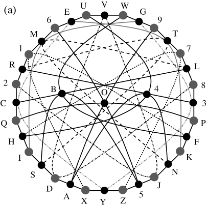
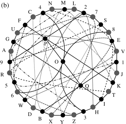
Figure 2: (a) OML with 35 atoms and 35 blocks that admits exactly one state: (35-35a) XYZ, Z5J, JNK, KFP, P38, 8L7, 7T9, 9GW, WVU, UE6, 6M1, 1R2, 2CQ, QHI, ISD, DAX, RST, OPQ, LMN, GIM, EKT, BCL, 9AO, 56O, 34R, 4AN, 5BS, BFW, 2JV, 4HU, 8DV, 7HZ, 3GY, 1FX, CEY.; (b) OML with 35 atoms and 35 blocks that is dual to itself and admits more than one state: (35-35e) XYZ, Z3H, HIT, TKJ, J1V, VE8, 8S7, 72L, LMN, N4C, CFU, UGA, A9R, R56, 6WD, DBX, UVW, RST, OPQ, GIQ, FKP, EIN, DKM, BCS, 46O, 38O, 15L, 3AM, 1BQ, 29P, 2HW, 4JY, 9EX, 7GY, 5FZ.  

The first two states found by our program are:

{(1)$\frac{1}{6}$,$\frac{1}{2}$,$\frac{1}{2}$,$\frac{1}{6}$,$\frac{1}{2}$,$\frac{1}{2}$,$\frac{1}{6}$,$\frac{1}{6}$,$\frac{1}{2}$,(A)$\frac{1}{2}$,$\frac{1}{6}$,$\frac{1}{6}$,$\frac{1}{2}$,$\frac{1}{6}$,$\frac{1}{2}$,$\frac{1}{6}$,$\frac{1}{2}$,$\frac{1}{6}$,(J)$\frac{1}{6}$,$\frac{1}{2}$,$\frac{1}{3}$,0,$\frac{2}{3}$,$\frac{1}{3}$,0,$\frac{2}{3}$,0,$\frac{2}{3}$,(T)$\frac{1}{3}$,$\frac{1}{3}$,$\frac{2}{3}$,0,$\frac{1}{3}$,$\frac{2}{3}$,(Z)0}

{(1)$\frac{1}{2}$,$\frac{1}{6}$,$\frac{1}{6}$,$\frac{1}{2}$,$\frac{1}{6}$,$\frac{1}{6}$,$\frac{1}{2}$,$\frac{1}{2}$,$\frac{1}{6}$,(A)$\frac{1}{6}$,$\frac{1}{2}$,$\frac{1}{2}$,$\frac{1}{6}$,$\frac{1}{2}$,$\frac{1}{6}$,$\frac{1}{2}$,$\frac{1}{6}$,$\frac{1}{2}$,(J)$\frac{1}{2}$,$\frac{1}{6}$,$\frac{1}{3}$,$\frac{2}{3}$,0,$\frac{1}{3}$,$\frac{2}{3}$,0,$\frac{2}{3}$,0,(T)$\frac{1}{3}$,$\frac{1}{3}$,0,$\frac{2}{3}$,$\frac{1}{3}$,0,(Z)$\frac{2}{3}$}where the values are for the aforementioned alphanumeric characters for the atoms in the above order from 1 to Z. Some atoms are indicated.

All other four 35-35 OMLs have exactly one state (1/3). One of them is drawn in Fig. 2(a). It has a mirror symmetry with respect to a vertical line drawn through atoms V,O,Y. The remaining 3 hypergraphs are given below. The reader can easily draw them since the first 16 blocks (chained) form a loop (hexadecagon). (35-35b) YXZ, Z3J, JTK, KNG, GU6, 65R, R9A, AWE, EMI, IFQ, Q2B, BCS, S87, 7O1, 1VH, H4Y, UVW, RST, OPQ, LMN, HIT, DKP, 48L, 36O, 25L, 3CM, 4AP, 19N, 2JW, CDV, 8FU, BGY, 9FZ, 7EX, 5DX. (35-35c) YXZ, ZFH, HIM, MLN, NKJ, J4S, SB3, 3P9, 91U, UVW, WTQ, QAG, GCE, E67, 7O2, 28Y, RST, OPQ, FGK, DEI, ABM, 89K, 5LP, 4HO, 5FR, 5DV, 4CU, 17R, 2BV, 8IT, 6NW, CLY, DJX, 1AX, 36Z. (35-35d) XYZ, ZFH, HIM, MLN, NJK, K8T, TWQ, QAE, EGC, C4U, U92, 2S7, 7P1, 1VB, BR3, 36X, UVW, RST, OPQ, FGK, DEI, ABN, 89I, 67G, 5LS, 4JP, 4HR, 5FO, 5DV, 39O, 6MW, CLY, DJX, 2AZ, 18Y.

There is only one 36-36 OML which is dual to itself and has only one state (1/3 for each atom). Its figure, that shows a cyclic (9) symmetry, is given in Fig. 2 of Ref. [14]. Here we write it down starting with 18 blocks that form the biggest loop (octadecagon). (36-36) XWY, YTS, SLP, PQ7, 7RO, OZJ, J5B, BN8, 82F, FCV, VH4, 416, 6IA, A9M, MK3, 3GU, UDE, EaX, NRX, MQW, LUZ, KVa, KOT, IPa, GHY, FWZ, BDQ, ACR, 9HJ, 8GI, 6DT, 5CS, 4LN, 29E, 135, 127.  

There are no 37-37 OMLs and there are eight 38-38 OMLs. Each one of the latter OMLs is dual to itself and they all have only one state (1/3). Using the programs we introduced in Ref. [13], we write them down so as to put the blocks that form the biggest loops [enneadecagons (19-gons) for the first seven and an octadecagon for the eighth] to the front (with chained blocks): (38-38a) abc, c12, 2L9, 98J, JHU, UPQ, QKS, SNO, O7Y, YXZ, ZWV, VA5, 5T4, 4MB, BCD, DIF, FEG, GR3, 36a, TUY, RSW, LMQ, IJW, AGH, EMZ, 69X, DKX, 3CP, 8CO, 46N, 7AL, 1FN, 1PV, 2RT, 5Kb, 8Eb, 7Ia, BHc. (38-38b) bac, cF3, 3SX, XI7, 7GV, VR1, 14L, LZM, M9T, TNO, OAW, WPQ, QJB, BCH, HDE, E5Y, Y2U, UK6, 68b, XYZ, UVW, RST, IJK, FGH, 8QZ, 6CS, 34P, 24N, 8GN, 9EP, ACL, 5JR, DIO, FKM, 1Db, 2Ba, 5Ac, 79a. (38-38c) abc, c65, 5ET, TZU, U1F, FGH, H4K, KLW, WIJ, J7C, CAB, BV9, 93N, NMY, YDP, POS, SQR, RX8, 82a, XYZ, VWZ, DEJ, 89E, 6SV, 7HX, 5AL, AGP, 2CM, 6FM, INQ, 2KO, 1LR, 4QT, 3OU, 1Db, GIa, 4Bb, 37c. (38-38d) cba, a95, 5FQ, QUP, PM2, 2AV, VWZ, ZYX, X47, 76E, E3T, TN8, 8IB, B1S, SDH, HJO, OKL, LRC, CGc, TUY, RSW, MNO, IJZ, GHU, DEF, CFI, 9AB, 7AG, 9LY, 5NW, 1MX, 3KV, 4KQ, 6PR, 13c, 2Db, 48b, 6Ja. (38-38e) acb, b59, 9SR, RG8, 83V, VWU, U1P, POY, YCN, NML, LQ2, 2FT, T7X, XAE, EDH, H6I, IKJ, JZB, B4a, XYZ, STW, QRZ, FGH, CKW, 9DN, 78M, 5AK, 4AL, BDV, 5FP, 1JM, 3IO, 6QU, 4OS, 23c, 67b, 1Ec, CGa. (38-38f) XZY, YTO, OA2, 24a, a13, 3E6, 6SH, HFb, b97, 7C8, 8QJ, JKW, WUV, VRP, PDM, MLN, NIB, Bc5, 5GX, abc, STW, QRZ, HIZ, FGV, DEY, BCT, 9AR, 56A, 48G, 2IU, 1KX, 1CP, 7EU, 9KN, FLO, 4MS, 3LQ, DJc. (38-38g) bac, c2J, JKY, YUT, T3D, DCE, EFR, R9H, HZI, I57, 7G6, 6XN, NOQ, QWP, P8A, A1L, LMS, SV4, 4Bb, XYZ, VWZ, RSU, FGW, 9AB, 8EK, 5PU, 3MQ, BGT, 2DV, 4KO, 1IO, 29N, 7JM, CLX, 5Cb, 68a, 1Fc, 3Ha. (38-38h) abc, c1K, KLX, XMN, N94, 43U, UZT, T6D, DGA, AVI, IJS, SPQ, QWO, O2H, H78, 8BF, FRC, C5a, XYZ, VWZ, RSY, GHY, EFW, CDL, 9AB, 6NQ, 57M, EJM, 3LO, 14R, BKP, 2JT, 17V, 5PU, 68b, 29a, EGc, 3Ib.  

Thus we obtain the following theorem.

Theorem 3.1.

There exist precisely $5$, $1$, $0$, and $8$ OMLs with $35$, $36$, $37$, and $38$ both atoms and blocks, respectively, and none of them admits a strong set of states.

4 Conclusion

In this elaboration we formulated a kind of reverse Kochen-Specker theorem that amounts to finding conditions imposed on a basic algebra of the Hilbert space as well as on Hilbert space vectors that cannot be satisfied by any quantum system. In 3-dim space this also applies to counterfactual orientation of experimental setups in the same way in which it works for Kochen-Specker setups. With the latter setups it is impossible to obtain consistent classical 0-1 measurement outcome and with our setups it is impossible to obtain consistent quantum outcomes.

Our “reversing of Kochen-Specker theorem” consists in generating basic quantum algebras—orthomodular lattices (OMLs)—that do not admit properties of the Hilbert space. There are many possible approaches to such a generation depending on what properties we want to consider. In this paper we decided to investigate the state properties of OMLs in a 3-dim space because states impose complex structures on ortholattice (algebra satisfying conditions (1)-(6) in Def. 2.1)—for instance an ortholattice with exactly one strong state is a Boolean algebra. Therefore we examined recent results—many of them reviewed in Mirko Navara’s review [16]—on orthomodular lattices with exactly one state.

Using MMP algorithms, we previously used to exhaustively generate Kochen-Specker vectors [11, 12], we obtained five smallest OMLs in 3-dim space with 35 atoms and 35 blocks (35-35), one 36-36, no 37-37, and eight 38-38. The smallest previously found such an OML has 44 atoms and 44 blocks. [19] OMLs that admit exactly one state have been previously investigated and used to obtain various properties of OMLs and related algebras and structures.[16] MMP diagrams (hypergraphs) and algorithms are briefly reviewed in Secs. 2 and 3 and in detail in the cited references. In 3D MMP for Hilbert vectors and OMLs amounts (at the level of bare vertices and edges).

Among five 35-35 OMLs we generated, four have exactly one state (1/3 for each atom) and the fifth, which is dual (with roles of atoms and blocks exchanged) to itself, has at least two states. The MMP diagrams (Greechie diagrams) of all five 35-35 OMLs are given in Sec. 2 as well as the states of the dual OML. We also provide figures of 35-35a with a single state and of the dual 35-35e in Fig. 2.

OML 36-36 is dual to itself and has exactly one state (1/3 for each atom). All of the 38-38s are dual to themselves and they all have exactly one state (1/3 for each atom). We give MMP (Greechie) diagrams for all of them Sec. 2.

We carried out several other tests on the aforementioned OMLs and obtained the following results:

• None of the obtained states belongs to a strong set of states, while it is apparently possible to have an OML admitting only one strong state as indicated by Pták results for posets [17]. Thus the former states are non-quantum (and therefore also non-classical), while the latter are classical (and therefore also quantum). Therefore we might view the former states as a kind of “reverse Kochen-Specker theorem” as explained in the Introduction.

• None of the generated OMLs pass any known stronger than orthomodularity condition as, e.g., Godowski equations (because they do not admit strong states) or orthoarguesian equations [29].

• OMLs that admit exactly one state that does not belong to a strong set of states are not limited only to those OMLs that have equal number of atoms and blocks as 73-78 given in footnote 4 proves. However, for lattices that have less blocks than atoms this is still an open question. We did not scan such lattices so far because that is computationally very demanding but it is one of our future projects.

• OMLs with equal number of atoms and blocks do not necessarily have only one state as dual 35-35e in Fig. 2(b) shows. Other duals, 36-36 and all 38-38, have only one state though.

We should stress here that the above OMLs with with exactly one state cannot be enlarged so as to become a sublattice of a Hilbert lattice because the orthoarguesian equations that have to hold in any Hilbert lattice fail in all above OMLs. And if an equation fails in a sublattice (meaning a subalgebra) it fails in the lattice as well.

To obtain further results both on bigger OMLs that admit only one state and on OMLs that do not admit other quantum conditions we are developing new algorithms some of which are presented in Ref. [15]. These algorithms will however not enable a generation of lattices with less blocks than atoms at all, so the aforementioned project of scanning lattices with less blocks than atoms will not make use of them.

We are developing new algorithms because the algorithms (gengre) we developed for generation of lattices with arbitrary number of atoms and blocks and used for obtaining Kochen-Specker vectors spend years of CPU time on our clusters. So, to go over 40 atoms and blocks we had to specialise the algorithms. [15]

In the end we should stress that our results also contribute to the theory of orthomodular lattices and to the theory of graphs and hypergraphs.

Acknowledgements

Supported by the Ministry of Science, Education, and Sport of Croatia through Distributed Processing and Scientific Data Visualization program and Quantum Computation: Parallelism and Visualization project (082-0982562-3160).

Computational support was provided by the cluster Isabella of the University Computing Centre of the University of Zagreb and by the Croatian National Grid Infrastructure.

References

- [1] S. Kochen and E. P. Specker, The problem of hidden variables in quantum mechanics, J. Math. Mech. 17, 59–87 (1967).
- [2] A. Peres, Two Simple Proofs of the Bell–Kochen–Specker Theorem, J. Phys. A 24, L175–L178 (1991).
- [3] J. Zimba and R. Penrose, On Bell Non-Locality without Probabilities: More Curious Geometry, Stud. Hist. Phil. Sci. 24, 697–720 (1993).
- [4] A. Cabello, Kochen–Specker Theorem and Experimental Tests on Hidden Variables, Int. J. Mod. Phys. A 15, 2813–2820 (2000).
- [5] M. Kernaghan, Bell–Kochen–Specker Theorem for 20 Vectors, J. Phys. A 27, L829–L830 (1994).
- [6] M. Kernaghan and A. Peres, Kochen–Specker Theorem for Eight-Dimensional Space, Phys. Lett. A 198, 1–5 (1995),
- [7] A. Cabello, J. M. Estebaranz, and G. García-Alcaine, Bell–Kochen–Specker Theorem: A Proof with 18 Vectors, Phys. Lett. A 212, 183–187 (1996).
- [8] A. Cabello and G. García-Alcaine, Proposed Experimental Tests of the Bell–Kochen–Specker Theorem, Phys. Rev. Lett. 80, 1797–1799 (1998).
- [9] A. E. Ruuge and F. Van Oystaeyen, Saturated Kochen-Specker-Type Configuration of 120 Projective Lines in Eight-Dimensional Space and its Group of Symmetry, J. Math. Phys. 46, 052109–1–28 (2005).
- [10] J. E. Massad and P. K. Aravind, The Penrose Dodecahedron Revisited, Am. J. Phys. 67, 631–638 (1999).
- [11] M. Pavičić, J.-P. Merlet, and N. D. Megill, Exhaustive Enumeration of Kochen–Specker Vector Systems, The French National Institute for Research in Computer Science and Control Research Reports RR-5388 (2004).
- [12] M. Pavičić, J.-P. Merlet, B. D. McKay, and N. D. Megill, Kochen–Specker Vectors, J. Phys. A 38, 497–503 (2005), J. Phys. A 38, 3709 (2005).
- [13] N. D. Megill and M. Pavičić, Equations, States, and Lattices of Infinite-Dimensional Hilbert Space, Int. J. Theor. Phys. 39, 2337–2379 (2000).
- [14] B. D. McKay, N. D. Megill, and M. Pavičić, Algorithms for Greechie Diagrams, Int. J. Theor. Phys. 39, 2381–2406 (2000).
- [15] M. Pavičić, B. D. McKay, N. D. Megill, and et al., In preparation (2008).
- [16] M. Navara, Small Quantum Structures with Small State Spaces, Int. J. Theor. Phys. 47, 36–43 (2008).
- [17] P. Pták, Exotic Logics, Coll. Math. 54, 1–7 (1987).
- [18] F. W. Shultz, A Characterization of State Spaces of Orthomodular Lattices, J. Comb. Theory A 17, 317–328 (1974).
- [19] M. Navara, An Orthomodular Lattice Admitting no Group-Valued Measure, Proc. Am. Math. Soc. 122, 7–12 (1994).
- [20] H. Weber, There Are Orthomodular Lattices without Non-Trivial Group Valued States; A Computer-Based Construction, J. Math. Anal. Appl. 183, 89–94 (1994).
- [21] M. Navara and V. Rogalewicz, Constructions for Orthomodular Lattices with Given State Spaces, Demonstratio Math. 21, 681–693 (1988).
- [22] M. Navara and V. Rogalewicz, State Isomorphism of Orthomodular Posets and Hypergraphs, in Proceedings of the 1st Winter School on Measure Theory, edited by A. Dvurečenskij and S. Pulmannová, pages 93–98, Liptovský Ján, Czechoslovakia, 1988, Slovak Academy of Sciences.
- [23] C. J. Isham, Lectures of Quantum Theory, Imperial College Press, London, 1995.
- [24] P. R. Halmos, Introduction to Hilbert Space and the Spectral Theory of Spectral Multiplicity, Chelsea, New York, 1957.
- [25] G. Kalmbach, Orthomodular Lattices, Academic Press, London, 1983.
- [26] P. Mittelstaedt, Quantum Logic, Synthese Library; Vol. 18, Reidel, London, 1978.
- [27] M. Pavičić, Nonordered Quantum Logic and Its YES–NO Representation, Int. J. Theor. Phys. 32, 1481–1505 (1993).
- [28] R. Mayet, Equational Bases for Some Varieties of Orthomodular Lattices Relatied to States, Algebra Universalis 23, 167–195 (1986).
- [29] M. Pavičić and N. D. Megill, Quantum Logic and Quantum Computation, in Handbook of Quantum Logic and Quantum Structures, edited by K. Engesser, D. Gabbay, and D. Lehmann, volume Quantum Structures, pages 751–787, Elsevier, Amsterdam, 2007.