Chameleon-Photon Mixing in a Primordial Magnetic Field
Abstract
The existence of a sizable, , cosmological magnetic field in the early Universe has been postulated as a necessary step in certain formation scenarios for the large scale magnetic fields found in galaxies and galaxy clusters. If this field exists then it may induce significant mixing between photons and axion-like particles (ALPs) in the early Universe. The resonant conversion of photons into ALPs in a primordial magnetic field has been studied elsewhere by Mirizzi, Redondo and Sigl (2009). Here we consider the non-resonant mixing between photons and scalar ALPs with masses much less than the plasma frequency along the path, with specific reference to the chameleon scalar field model. The mixing would alter the intensity and polarization state of the cosmic microwave background (CMB) radiation. We find that the average modification to the CMB polarization modes is negligible. However the average modification to the CMB intensity spectrum is more significant and we compare this to high precision measurements of the CMB monopole made by the far infrared absolute spectrophotometer (FIRAS) on board the COBE satellite. The resulting 95% confidence limit on the scalar-photon conversion probability in the primordial field (at ) is . This corresponds to a degenerate constraint on the photon-scalar coupling strength, , and the magnitude of the primordial magnetic field. Taking the upper bound on the strength of the primordial magnetic field derived from the CMB power spectra, , this would imply an upper bound on the photon-scalar coupling strength in the range to , depending on the power spectrum of the primordial magnetic field.
I Introduction
The origin of the observed large-scale magnetic fields of order found in nearly all galaxies and galaxy clusters is still largely unknown. It is generally believed that the galactic magnetic field develops by some form of amplification from a pre-galactic cosmological magnetic field. The two popular formation scenarios that are considered are either some exponential dynamo mechanism which amplifies a very small seed field of order as the galaxy evolves, or the adiabatic collapse of a larger existing cosmological field of order . There are a number of pros and cons to both scenarios. See Kronberg94 for reviews on the subject. Theories explaining the origin of this primordial magnetic (PMF) field are still highly speculative. It has been suggested that a large-scale magnetic field could be produced during inflation if the conformal invariance of the electromagnetic field is broken; see for example Ratra92 or more recently Kunze10 .
To date, there is no astrophysical evidence for the existence of a large-scale cosmological magnetic field, and only upper bounds on its magnitude have been derived. So far the strongest constraints have come from measurements of the cosmic microwave background (CMB) and big-bang nucleosynthesis Kronberg94 ; Tashiro06 ; Kosowsky09 ; Yamazaki10 ; Paoletti10 . The CMB bounds are derived by considering the effects of Faraday rotation induced by the PMF on the CMB power spectra. In Kosowsky09 an upper limit in the range to was derived for the mean-field amplitude of the PMF at a comoving length scale of by comparison to the WMAP 5-year data. More recent work Yamazaki10 ; Paoletti10 analysing the WMAP data in combination with other CMB experiments such as ACBAR, CBI and QUAD have placed tighter constraints on the amplitude of the PMF with an upper bound on the mean-field amplitude at of .
The existence of a primordial magnetic field would induce mixing between CMB photons and axion-like particles (ALPs). ALPs refer collectively to any very light scalar or pseudo-scalar with a linear coupling to or respectively. In this paper we consider non-resonant mixing of scalar ALPs and CMB photons, with specific reference to the chameleon scalar field model Khoury04 ; Brax07 ; Burrage08 . Standard ALPs have constant mass and photon-scalar coupling everywhere, while the chameleon model has a density dependent mass. In sparse environments, such as the primordial plasma, the chameleon acts as a very light scalar field and would be indistinguishable from a standard scalar ALP. However in dense environments the chameleon is very heavy and evades the standard ALP constraints Brax09 . The current best constraints on the coupling strength between the chameleon and electromagnetic fields are: Burrage08 and Davis09 . Other chameleon-like theories exist such as the Olive-Pospelov model Davis09 ; Olive08 which have a density-dependent coupling strength, but we do not discuss these further here.
The resonant mixing of photons with scalar and pseudo-scalar ALPs in a primordial magnetic field has been analysed by Mirizzi, Redondo and Sigl Mirizzi09 . They find a constraint on the combined magnetic field strength, , and ALP-photon coupling strength, : , for ALP masses between and . We believe that these results will not necessarily be applicable to the chameleon because its mass evolves as the density of the Universe decreases.
In the following analysis we assume a stochastic primordial magnetic field with a power-law power spectrum, similar to the treatment in Kosowsky09 . We assume fluctuations in the magnetic field are damped on small scales due to Alfvn wave dissipation Barrow98 , and subdivide the magnetic field into multiple domains of length of a comparable size to just above the Alfvn wave damping scale . The magnetic field in each domain is assumed to be approximately constant, and correlated to the other domains according to the magnetic power spectrum. A similar method was applied to correlations in quasar polarization spectra by Agarwal, Kamal and Jain Agarwal09 .
The degree of conversion between chameleons and photons in a magnetic field is inversely proportional to the electron density in the plasma Davis09 . Hence the dominant contribution to photon-scalar mixing will take place in the region after recombination when the ionization fraction drops significantly and before reionization. This greatly simplifies the mixing equations because we do not need to evolve the photon-scalar mixing equations through the last scattering surface, nor include the density inhomogeneities present after reionization. We model a scenario in which the primary CMB is formed at the last scattering surface and then evolves through a primordial magnetic field extending from recombination () to the epoch of reionization ().
This paper is organized as follows: in section II the chameleon model is introduced and the calculations describing photon-scalar mixing in a magnetic field, living in a Friedman-Robertson-Walker (FRW) spacetime, are presented. The power spectrum of the primordial magnetic field is discussed in more detail in section III. In section IV we analyse the evolution of the photon and chameleon states as they propagate through the multiple magnetic domains, and predict the average modification to the CMB intensity and polarization. In section V, our predictions are compared to precision measurements of the CMB monopole made by the far infrared absolute spectrophotometer (FIRAS) on board the cosmic background explorer (COBE) satellite. We present a summary of the work and our conclusions in section VI. The appendix contains details of the equations governing the evolution of the CMB Stokes parameters.
II Chameleon-Photon Mixing in an Expanding Universe
The chameleon scalar field has been suggested as a candidate for the dark energy quintessence field Khoury04 . Standard quintessence scalar fields have coupling strengths to matter which are unnaturally fine-tuned to very low values so as to be compatible with fifth-force experiments. By contrast the chameleon model is constructed so that the chameleon can have a gravitational strength (or greater) coupling to normal matter while at the same time evading fifth-force constraints. This is achieved by introducing a density-dependent term in the effective potential of the chameleon, which causes a change to the minimum of the potential depending on the density of the surrounding matter. In sparse environments the chameleon behaves as an effectively massless scalar field while in a laboratory on Earth it is much heavier and evades detection.
In addition to the matter coupling, the chameleon can have a non-zero coupling, , to the electromagnetic (EM) field. The mass parameter, , describing the strength of the photon coupling is best constrained by observations of radiation passing through astrophysical magnetic fields. The two best current constraints in terms of the coupling strength were presented in section I. In terms of , the lower limit from considering constraints on the production of starlight polarization in the galactic magnetic field is Burrage08 . Measurements of the Sunyaev–Zel’dovich effect in galaxy clusters places a lower bound on in the range to , depending on the model assumed for the cluster magnetic field Davis09 .
The action describing the chameleon model is that of a generalized scalar-tensor theory:
where is the self-interaction potential of the scalar field , and is the matter action, excluding the kinetic term of electromagnetism, which contains the coupling of the matter fields to the conformal metric . The determine the coupling of the scalar field to different matter species, and determines the photon-scalar coupling. For simplicity a universal matter coupling, , is assumed. We take the Universe to be described by a spatially-flat Friedman-Robertson-Walker (FRW) metric: where is the time-dependent scale factor describing the expansion, normalized to today. The coordinates are comoving, related to the physical coordinates by , and is the proper time.
The equation of motion for the field is found by varying with respect to :
where is the Hubble expansion rate. is the trace of the stress-energy tensor in the conformal frame described by the metric , for which particle masses are constant and independent of . This is related to the stress-energy tensor in the physical frame by . In general, corresponding to the physical, measured density and pressure. If we assume the chameleon does not couple to the energy density of dark matter or any other exotic particles, then , the baryonic matter density. Hence
where,
The form of the self-interaction potential determines whether a general scalar-tensor theory is chameleon-like or not. For a chameleon field we require the potential to be of runaway form. A typical choice of potential can be described by
| (1) |
where for reasons of naturalness . If the chameleon is to be a suitable candidate for dark energy, we require . The chameleon mass is defined by
where is the background value of the electromagnetic field tensor.
The photon equation of motion comes from varying with respect to :
Any electromagnetic components in would introduce electromagnetic currents on the right-hand side of the equation. We neglect these at this stage in the calculation. The primordial plasma is a good conductor and so any currents will be small Barrow07 . To a good approximation the induced currents arising from photon propagation will be described by the plasma frequency which is included later in this calculation.
In standard chameleon theories we assume and approximate and , where this defines and . We expect these two coupling strengths to be of similar magnitude but do not require it. Under this approximation, and splitting the electromagnetic field into the background EM field and the photon field , the above equations of motion become
where is the perturbation in the scalar field about its background value, and we neglect terms that are and .
In an inertial, locally Minkowskian frame, with metric , the electromagnetic field tensor has the form
The coordinate transformation from the locally Minkowski metric, , into the FRW metric, , is
with
Thus in an FRW expanding Universe the EM field tensor is given by
We take the background to be a large-scale magnetic field , and assume the contributions from electric fields in the plasma are negligible. The photon field can be described by the quantum polarization states where . Taking the Lorentz gauge condition , we find the equations of motion become
and
where we define the deceleration parameter, .
In this analysis we have assumed that the background values of the chameleon and photon fields are slowly varying over length and time scales of where is the proper frequency of the electromagnetic radiation being considered. We further assume that the frequency of the radiation satisfies and that . The equations describing mixing between the photons and scalar field are then
where we have included the plasma frequency, , as an effective photon mass. Whenever electromagnetic radiation propagates through a plasma with electron number density it displaces the electrons slightly and induces oscillations at their natural frequency . This interaction of the EM wave with the electron density hinders its progress and acts as an effective mass for the photons.
Taking the radiation to be propagating in the direction of an orthonormal Cartesian basis , with , the equations of motion for the chameleon and photon can be written in matrix form:
Note how the chameleon scalar field only mixes with the component of photon polarization aligned perpendicular to the transverse magnetic field. The magnitude of the magnetic field aligned parallel to the photon path () plays no part in the mixing.
Following a similar procedure to that in Davis09 ; Raffelt88 we assume the fields vary slowly over time compared to the frequency of the radiation and that the refractive index is close to unity, which requires , and all . Defining and , we approximate and such that . Thus,
We further simplify the mixing matrix by defining and with . The magnetic field and frequency can be expressed in terms of their comoving values: and . In the subsequent analysis we drop the subscript-zero notation for comoving magnetic field values. Thus we can write
| (8) |
where .
To solve this system of equations we must make various simplifying assumptions. We neglect spatial fluctuations in the electron density along the path length, and only consider a simple redshift scaling: , where is the ionization fraction along the path. The ionization fraction drops rapidly at recombination from to its final freeze-out value Seager99 , and only increases again at the epoch of reionization. The conversion between photons and light scalar particles in a magnetic plasma scales inversely with the electron number density in the plasma Davis09 . Thus the conversion will be suppressed for high values of the ionization fraction. We assume the dominant contribution to photon-scalar mixing in a primordial magnetic field occurs between redshift (by which time the ionization fraction has already dropped to ) and redshift (onset of reionization). We approximate the ionization fraction as being at a constant value of in this region, and neglect contributions from other sections of the path length.
The chameleon mass for the generalized self-interaction potential of Eq. (1) is
where the second line assumes , a magnetic field of less than , a chameleon coupling strength of less than , and that the average baryonic density is 4% of the critical density. We compare this to the plasma frequency,
over the redshift range to 750, where we have taken the average mass per baryon to be Steigman06 . It is clear then that along the path from recombination to reionization. Our subsequent analysis requires the chameleon to be sufficiently light for the plasma frequency to dominate over the path length, and thus is not dependent on the specific form of the chameleon potential. It applies to any scalar ALP satisfying this condition.
The comoving distance, , travelled by the photons is related to the value of the scale factor at by
This leads to
in the matter dominated era between recombination and reionization, where Dunkley08 . Over the total path length from a redshift of to , the comoving distance covered is .
Changing the integration variable in Eq. (8) to
such that , and noting , we find
| (15) |
where . The –dependence of the mixing matrix is entirely due to fluctuations in the magnetic field.
III The Primordial Magnetic Field
The generic model for the primordial magnetic field is of a stochastic field parameterized by a power-law power spectrum up to a cut-off scale ,
where is some normalization constant. The spectral index must be greater than to prevent infrared divergences in the integral over the power spectrum at long wavelengths. Assuming a statistically homogeneous and isotropic field, the power spectrum is defined by
where is the projector onto the transverse plane imposed by the divergence-free nature of the magnetic field. We adopt the Fourier transform convention,
The two-point correlation function is then
Following the prescription in Kosowsky09 ; Kosowsky05 , normalization of the magnetic field is achieved by convolving the field (in real space) with a Gaussian smoothing kernel of comoving radius . Defining the Fourier transform of the Gaussian smoothing kernel to be , the Fourier transform of the convolved field is
The mean-field amplitude of the smoothed field, , is given by
Hence the normalization constant,
where .
Constraints on the magnitude of the primordial magnetic field from a comparison of Faraday rotation effects in the CMB with the WMAP 5-year data were given in Kosowsky09 . They found that the upper limit on the mean-field amplitude of the magnetic field on a comoving length scale of was in the range to () for a spectral index to . This range for the spectral index was based on the likely formation scenarios for the primordial magnetic field Ratra92 and current exclusion bounds on the spectral index Caprini01 . More recent results analysing the WMAP 5-year data in combination with other CMB experiments Yamazaki10 constrained the mean-field amplitude and the spectral index (). An analysis of the latest WMAP 7-year data Paoletti10 derived upper bounds of and ().
The magnetic field power spectrum will be damped at small length-scales. We assume a cut-off to the power spectrum at the Alfvn wave damping scale Barrow98 . This damping scale is approximated Kosowsky05 as
where .
Using these definitions, we can calculate the correlations in the magnetic field along the line of sight:
where we have written the wave vector in spherical polar coordinates, . Thus
and
where
Substituting the assumed form for the magnetic power spectrum, and changing variables, we find
| (16) |
with
| (17) |
IV Evolution of the Stokes Parameters
Following a similar procedure to that in Agarwal09 we subdivide the path length into many small domains of length , each with a constant magnetic field strength and direction, and take correlations in the field across the different domains to be described by the magnetic power spectrum. The inverse power-law form assumed for the primordial magnetic power spectrum imposes a rapidly decreasing amplitude to the field fluctuations and an even faster decreasing slope to the magnetic power spectrum with increasing . At very large the amplitude of the fluctuations are damped to zero by Alfvn wave dissipation. However slightly above the Alfvn wave damping scale, , the amplitude of the field is non-zero yet the slope of the power spectrum will be approximately flat. In what follows we assume on scales slightly greater than the magnetic field can be approximated as constant and take . The exact value of is only necessary in determining the number of magnetic domains that the photons traverse along the path. Some variation in will not affect the order of magnitude of the final results.
IV.1 Evolution through a Single Domain
For a single domain we define to be the magnitude of the transverse component of the magnetic field, and to be the angle it makes with the -axis. Within the domain these stay approximately constant. Returning to Eq. (15), we rotate the basis so as to reduce the problem to two-component mixing. Defining
we find is constant over the domain and
Diagonalisation of this two-component mixing leads to
where
and
| (18) | |||||
| (19) |
Additionally defining
the chameleon and photon polarization states in the rotated basis after passing through a single domain of length , are
where and . The probability of conversion between chameleons and photons in a single domain is .
The intensity and polarization state of radiation is best described by its Stokes parameters: intensity, , linear polarization, and , and circular polarization, . These are defined in terms of the photon polarization states by
We additionally define chameleon ‘Stokes parameters’ to close the evolution equations,
The evolution of the Stokes parameters through a single magnetic domain, in the rotated basis, is then
and
is found by requiring that the total flux of photons and chameleons along the path length is conserved, .
IV.2 Evolution through Multiple Magnetic Domains
The evolution equations above can be extended to many domains following a similar procedure to that in Burrage08 .
For CMB photons in the range , passing through a magnetic field of less than , and assuming a photon-scalar coupling strength no greater than , the mixing parameters defined in Eqs. (18) and (19) satisfy and in a domain of length . There is a region towards the end of the path at larger for which , but the approximations that follow involving averaging terms in and along the path are still valid in this instance. Thus on average over the total path length,
This places us in the regime of weak-mixing which can be solved analytically if we neglect terms smaller than , where is the number of magnetic domains along the path. Details of the mixing equations in multiple domains are presented in the Appendix. Here we quote the average, over many lines of sight, of the modification to the Stokes parameters. We assume there is no initial flux of chameleons and define to be the location of the domain. Then,
where was defined in Eq (16). Over the range to , the integral (Eq. (17)) can be well approximated by a window function: for , and zero otherwise. Taking the domain length , the average modification to the CMB intensity is then
| (20) |
where we have averaged terms in and , since . Of the average modifications to the Stokes parameters, that of the CMB intensity will be most significant since the CMB is only weakly polarized with .
In addition to the average modification to the Stokes parameters as a result of photon-scalar mixing, there will also be a change to the correlations between different Stokes parameters. A full derivation of the cross-correlations along different lines of sight would require us to expand the primordial field power spectrum in spherical harmonics, a task we reserve for a future paper Schelpe10 . However we can estimate the magnitude of the effect by looking at, say, the cross-correlation along the line of sight. The dominant contribution, neglecting terms proportional to , and smaller, is
From this we see that a significant correlation can arise from the much larger correlation. Although the above analysis only applies to the average correlations along many lines of sight, for which in the CMB, we expect a similar magnitude to the effect when a full derivation for the cross-correlations along different lines of sight is made. It opens up the exciting possibility of a significant chameleon contribution to the power spectrum of the CMB.
V Bounds on the CMB Intensity from FIRAS
Returning to Eq. (20), we have that the average modification to the CMB intensity from scalar-photon mixing in a primordial magnetic field is
where we have defined
This expresses the primordial magnetic field in terms of its mean-field amplitude, , at a length-scale of . Most constraints on the magnitude of the magnetic field are expressed in terms of these parameters. The value of dictates the slope of the magnetic power spectrum, and we consider the range to .
The most precise measurements to date of the CMB monopole near the peak in its spectrum come from the far infrared absolute spectrophotometer (FIRAS) on board the cosmic background explorer (COBE) satellite Fixsen96 ; Fixsen02 . These measurements fit exceptionally closely to the spectrum of a black-body at a temperature of . In Table 4 of Fixsen96 , the residuals of the CMB monopole that remain after subtracting foreground effects are listed. These residuals, added to the spectrum of a perfect black-body radiating at , can be compared to the predictions of photon-scalar mixing to constrain the parameter space. The FIRAS instrument has 43 significant frequency channels in the range after calibration. The spectral intensity of a black-body at temperature is
In the presence of photon-scalar mixing the spectrum is modified to
| (21) |
where is defined such that
We maximize the likelihood, , defined by
over the parameter space . Here is the observed CMB monopole measured by FIRAS at 43 different frequencies, , with standard errors . is the spectral intensity predicted for chameleon-photon mixing given in Eq (21). We treat as a free parameter in our analysis rather than fixing it at . Confidence limits are estimated by assuming
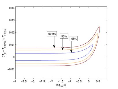
follows a distribution, where are the best fit values of and in the parameter space, found by the maximum likelihood procedure. Minimizing with respect to gives , identical to the value obtained when no chameleon mixing is considered. Minimizing with respect to gives the following 95% confidence limit on ,
Fig. 1 shows the 68%, 95% and 99.9% confidence limits on the parameter space.
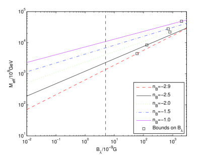
The limit on corresponds to a degenerate constraint on the magnitude of the primordial magnetic field and the chameleon-photon coupling strength. The magnetic field strength is expressed in terms of the mean-field amplitude at a comoving length-scale of , . In Fig. 2 we plot the exclusion bounds in the parameter space resulting from the 95% confidence limit on . Different lines correspond to different values of the magnetic spectral index, , in the range -2.9 to -1. The open squares mark the 95% upper limit on the allowed values for (for each ) found in Kosowsky09 from comparison of Faraday rotation effects in the CMB with WMAP 5-year data. The vertical line corresponds to the more recent constraints on given in Yamazaki10 and Paoletti10 . The region to the bottom right of the plot for each value is excluded at the 95% confidence level. For example if we take a magnetic field strength at the upper limit allowed by Faraday rotation effects in the CMB, , the corresponding bound on the photon-scalar coupling strength, , is
depending on the slope of the magnetic power spectrum.
VI Conclusions
The existence of a large-scale cosmological field in the early Universe is so far unconfirmed. It would need to be in the region of if it is to explain the formation of the magnetic fields in galaxies and galaxy clusters, through adiabatic collapse. If this primordial magnetic field exists it would induce mixing between CMB photons and axion-like particles (ALPs) as they propagate from the last-scattering surface to Earth.
In this paper we have studied the case of non-resonant mixing between scalar-ALPs and photons in a primordial magnetic field, with specific reference to the chameleon scalar field model.
The chameleon model is a promising candidate for the dark energy scalar field since it can have a gravitational strength (or stronger) coupling to normal matter while at the same time evading fifth-force constraints. To date, the strongest bounds on the chameleon coupling strength come from chameleon-photon mixing in local astrophysical environments, such as starlight propagating through the galactic magnetic field: Burrage08 . Should there be a detection of a primordial magnetic field of order , our results would place far greater constraints on the coupling strength.
We have considered a stochastic primordial magnetic field described by a power-law power spectrum, , up to some cut-off damping scale . Photon-scalar mixing in this field was solved by dividing the path length into multiple magnetic domains in which the field is approximated as constant. The length of the domains was taken to be of a comparable size to since the magnetic power spectrum will be approximately flat, but non-zero, just above the damping scale. Correlations between the magnetic field strength and direction in each domain are determined by the magnetic power spectrum. In addition, we approximated the ionization fraction as being constant in the region from redshift to , and held at its post-recombination freeze-out value of . The dominant contribution to photon-scalar mixing in the CMB will occur in this region of low electron density, and we neglected contributions from other elements of the path length. A more sophisticated approach to modelling the electron density from recombination to the present day may result in small changes to the predictions, but would require a numerical rather than analytical approach to the mixing equations.
We have compared our predictions of the average modification of the CMB intensity over the whole sky, to precision measurements of the CMB monopole by the FIRAS instrument on board the COBE satellite Fixsen96 ; Fixsen02 . This constrains the probability of photon-scalar mixing over the path length, to be
at . The corresponding bounds on the magnitude of the magnetic field and photon-scalar coupling strength are plotted in Fig. 2 for different values of the magnetic spectral index. Until a detection of the primordial magnetic field is made, to break the degeneneracy of this constraint, we cannot place limits on the chameleon-photon coupling strength, . For the largest magnetic field allowed by the constraints in Yamazaki10 ; Paoletti10 we would find the strongest possible constraint,
depending on the slope of the magnetic field power spectrum.
The results in this paper apply to any scalar ALP with a mass less than , since we require the mass to be much smaller than the plasma frequency along the path. These nicely complement the bounds derived in Mirizzi09 for resonant conversion between photons and ALPs in a primordial magnetic field, , which apply to ALP masses in the range to .
In addition to the average modification to the CMB intensity, the formalism developed in this paper can straightforwardly be extended to calculate the change to correlations between the CMB Stokes parameters along different lines of sight. In section IV.2, an example was given of how a correlation between the and polarization modes can arise from photon-scalar mixing in the primordial magnetic field, given a non-zero correlation. If this effect is present in the CMB cross-correlations, it would lead to a significant chameleon signature in the power spectrum. A full analysis of this effect is kept for a separate publication Schelpe10 .
Acknowledgments: I am funded by STFC. I am grateful to Douglas Shaw and my supervisor Anne Davis for their support, and to Anthony Challinor for interesting and helpful discussions.
Appendix A Photon-Scalar Mixing in Multiple Magnetic Domains
In section IV.1 we found the evolution equations of the Stokes parameters after passing through a single magnetic domain of length , within which the magnetic field strength and direction are approximated as constant. This can be extended to multiple domains, under the assumption of weak-mixing for which we require and . CMB photons in the range , propagating through a weak primordial magnetic field, satisfy and . In this limit , and . We define to be the difference in intensity after passing through the domain compared to its initial value, , and similarly for the other parameters. Neglecting terms smaller than , we obtain the following recurrence relations for the Stokes parameters:
with
where we have assumed there is no initial chameleon flux which necessarily sets . Note that depends on the magnitude of the transverse component of the magnetic field, which fluctuates over the different domains, hence the subscript , whereas is constant along the path save for a weak dependence on the scale factor. However, since , this will be averaged out across the path length. Solving this system of equations for propagation through domains, we find the modified Stokes parameters:
where we have defined
and
and
and
We define to be the location of the domain, then and by definition. Remembering , we find that the average over many lines of sight of the above quantities are
and all other quantities average to zero. We have assumed fluctuations in the magnetic field are approximately Gaussian so that the four-point correlations can be expressed in terms of the two-point correlation function, , defined in Eq. (16).
Taking the average of the modified Stokes parameters, over the whole sky, we find
References
- (1) P.P. Kronberg, Rept. Prog. Phys. , 325-382 (1994); C. Carilli and G. Taylor, Ann. Rev. Astron. Astrophys. , 319 (2001); L.M. Widrow, Rev. Mod. Phys. , 775-823 (2002); R.M. Kulsrud and E.G. Zweibel, Rept. Prog. Phys. , 0046091 (2008).
- (2) M.S. Turner and L.M Widrow, Phys. Rev. D37, 2743 (1988); B. Ratra, Astrophys. J. , L1-L4 (1992); M. Gasperini, M. Giovannini and G. Veneziano, Phys. Rev. D52, 6651-6655 (1995); O. Bertolami and D.F. Mota, Phys. Lett. B455, 96-103 (1999).
- (3) K.E. Kunze, Phys. Rev. D81, 043526 (2010); T. Kahniashvili , .
- (4) H. Tashiro, N. Sugiyama and R. Banerjee, Phys. Rev. D, 023002 (2006); T. Kahniashvili, A.G. Tevzadze and B. Ratra, .
- (5) T. Kahniashvili, Y. Maravin and A. Kosowsky, Phys. Rev. D, 023009 (2009).
- (6) D.G. Yamazaki, K. Ichiki, T. Kajino and G.J. Mathews, Phys. Rev. D, 023008 (2010).
- (7) D. Paoletti and F. Finelli, .
- (8) J. Khoury and A. Weltman, Phys. Rev. Lett. , 171104 (2004); Phys. Rev. D, 044026 (2004).
- (9) P. Brax, C. van de Bruck, A.C. Davis, Phys. Rev. Lett. 99, 121103, (2007); P. Brax, C. van de Bruck, A.C. Davis, D.F. Mota and D. Shaw, Phys. Rev. D, 085010 (2007); C. Burrage, Phys. Rev. D, 043009 (2008).
- (10) C. Burrage, A.C. Davis and D.J. Shaw, Phys. Rev. D, 044028 (2009).
- (11) P. Brax, C. van de Bruck, A.C. Davis and D. Shaw, ; G.G. Raffelt, Lect. Notes Phys. 741, 51 (2008); D.F. Mota and D.J. Shaw, Phys. Rev. Lett. 97 151102 (2006); D.F. Mota and D.J. Shaw, Phys. Rev. D.75, 063501 (2007).
- (12) A.C. Davis, C.A.O. Schelpe and D.J. Shaw, Phys. Rev. D, 064016 (2009).
- (13) K.A. Olive and M. Pospelov, Phys. Rev. D77, 043524 (2008); D.F. Mota and J.D. Barrow, Phys. Lett. B581, 141-146 (2004); D.F. Mota and J.D. Barrow, Mon. Not. Roy. Astron. Soc. , 291 (2004).
- (14) A. Mirizzi, J. Redondo and G. Sigl, JCAP , 001 (2009).
- (15) K. Jedamzik, V. Katalinic and A.V. Olinto, Phys. Rev. D, 3264-3284 (1998); K. Subramanian and J.D. Barrow, Phys. Rev. Lett. , 3575-3578 (1998).
- (16) N. Agarwal, A. Kamal and P. Jain, .
- (17) J.D. Barrow, R. Maartens and C.G. Tsagas, Phys. Rept. , 131-171 (2007).
- (18) G. Raffelt and L. Stodolsky, Phys. Rev. D 37 1237 (1988).
- (19) S. Seager, D.D. Sasselov and D. Scott, Astrophys. J. Suppl. , 407-430 (2000); A. Lewis, J. Weller and R. Battye, Mon. Not. Roy. Astron. Soc. , 561-570 (2006).
- (20) G. Steigman, JCAP , 016 (2006).
- (21) WMAP Collaboration, G. Hinshaw , Astrophys. J. Suppl. , 225 (2009).
- (22) A. Kosowsky, T. Kahniashvili, G. Lavrelashvili and B. Ratra, Phys. Rev. D, 043006 (2005); A. Mack, T. Kahniashvili and A. Kosowsky, Phys. Rev. D, 123004 (2002).
- (23) C. Caprini and R. Durrer, Phys. Rev. D, 023517 (2001).
- (24) C.A.O. Schelpe, in preparation.
- (25) D.J. Fixsen , Astrophys. J. , 576 (1996).
- (26) D. J. Fixsen and J.C. Mather, Astrophys. J. , 817-822 (2002); J.C. Mather , Astrophys. J. , 511-520 (1999).