Fast magnetic reconnection
in three dimensional MHD simulations

Abstract

We present a constructive numerical example of fast magnetic reconnection in a three dimensional periodic box. Reconnection is initiated by a strong, localized perturbation to the field lines. The solution is intrinsically three dimensional, and its gross properties do not depend on the details of the simulations. $\sim 50\%$ of the magnetic energy is released in an event which lasts about one Alfven time, but only after a delay during which the field lines evolve into a critical configuration. We present a physical picture of the process. The reconnection regions are dynamical and mutually interacting. In the comoving frame of these regions, reconnection occurs through an X-like point, analogous to Petschek reconnection. The dynamics appear to be driven by global flows, not local processes.

I Introduction

Most of the matter in the universe exists in the plasma state and plasma also plays an important role in gas dynamics in astrophysics. When magnetic field are present, the dynamics of an electrically conducting plasma is sensitive to magnetic forces; as a result, magnetohydrodynamics(MHD) is used to understand the dynamical evolution of astrophysical fluids.

The ideal limit of MHD poses a new class of problems in dissipative processes. In ideal hydrodynamics, irreversible processes, such as shock waves and vorticity reconnection, occur at dynamical speeds, independent of microscopic viscosity parameters. Weak solutions describe these irreversible discontinuous solutions of the Euler equations. While smooth flows conserve entropy and vorticity, the infinitesimal discontinuity surfaces generate entropy and reconnect vorticity. This can also be understood as a limiting case starting with finite viscosity, where these surfaces have a finite width.

With magnetic fields, a more dramatic problem emerges. If two opposing field lines sit nearby, a state of higher entropy can be reached by reconnecting the field lines, and converting their magnetic energy into fluid entropy. In the presence of resistivity, this process occurs on a resistive time scale for some relevant scale. This exaggerates the problem somewhat. Extensive theoretical research on magnetic reconnection(Biskamp (2000), Priest and Forbes (2000)) has shown that scales intermediate between the size of a system and resistive scales can be important. Nevertheless, in many astrophysical settings, simple models for reconnection give time scales that are very long, and reconnection is observed or inferred to occur on much shorter time scales, e.g. for solar flares, more than $10^{10}$ times faster than the theoryDere et al. (1991). This has led to the suggestion that magnetic reconnection in the limit of vanishing resistivity might also go to a weak (discontinuous) solution, occuring at a finite speed which is insensitive to the value of the resistivity.

The problem is best illustrated by the Sweet-Parker configuration (Sweet (1958), Parker (1957)), where opposing magnetic fields interact in a thin current sheet, the reconnection layer. This unmagnetized layer becomes a barrier to further reconnection. In a finite reconnection region, fluid can escape the reconnection region at alfvenic speeds. Because the reconnection region is thin, the reconnection speed is reduced from the alfven speed by a factor of the ratio of the current sheet width to the transverse system size. In the Sweet-Park model this factor is the inverse of the square root of the Lundquist number ($V_{A}L/\eta$). The predicted sheet widths are typically extremely thin.

Petschek proposed a fast magnetic reconnection solution (Petschek (1964)) based on the idea that magnetic reconnection happens in a much smaller diffusive region, called the X-point, instead of a thin sheet. The global structure is determined by the log of the Lundquist number, and stationary shocks allow the fluid to convert magnetic energy to entropy.

However, Biskamp’s simulations (Biskamp (1986)) showed that Petschek’s solution is unstable when Ohmic resistivity becomes very small. In their two dimensional incompressible resistive MHD simulations, they injected and ejected plasma and magnetic flux across the boundary. They also changed the boundary condition during the simulation to eliminate the boundary current layer. However, considering the current sheet formed in their simulation, the computation domain may not be big enough. After reproducing different scaling simulations results(Biskamp (1986), Lee and Fu (1986)), Priest and Forbes Priest and Forbes (1992) pointed out that it is the boundary conditions that determine what happens (including Biskamp’s unstable Petscheck’s simulation) and that sufficiently free boundary conditions can make fast reconnection happen. However, there is no self-consistent simulation of fast reconnection reported, except with artificially enhanced local resistivityScholer (1989).

To reconcile the observed fast reconnection with its absence in simulations leads to two possible resolutions: 1) ideal MHD are not the correct equations, and long range collisionless effects are required, or 2) assumptions about the reconnection regions are too restrictive. This includes the 2-dimensionality and the boundary conditions.

In exploring of the first possibility, it was found that when integrating with the Hall term in the MHD equations, or using a kinetic description(Birn et al. (2001)), it was possible to find fast reconnection. However, this still didn’t offer any help to the collisional system, which still has fast magnetic reconnection no matter whether Hall term is present or not; and also the increase of local resistivity is not generic in astrophysical environments, which mostly has highly conducting fluids.

For the second possibility, we note that Lazarian & Vishniac (LV99) Lazarian and Vishniac (1999) proposed a model of fast magnetic reconnection with low amplitude turbulence. Subsequent simulation results Kowal et al. (2009) support this model. They found that the reconnection rate depends on the amplitude of the fluctuations and the injection scale, and that Ohmic resistivity and anomalous resistivity do not affect the reconnection rate. The result that only the characteristics of turbulence determine the reconnection speed provides a good fit for reconnection in astrophysical systems.

LV99 offered a solution to fast magnetic reconnection in collisional systems with turbulence. In this paper, we consider a different problem, whether we could still have fast reconnection without turbulence. We present an example of fast magnetic reconnection in ideal three dimensional MHD simulation in the absence of turbulence. Here we explore a different aspect: 3-D effects and boundary conditions. Traditionally, simulations have searched for stationary 2-D solutions, or scaling solutions. In the case of fast reconnection, the geometry changes on an alfvenic time, so these assumptions might not be applicable. Specifically, we bypass the choice of boundary condition by using a periodic box.

The primary constructive fast reconnection solution, the Petscheck solution, has some peculiar aspects. The global geometry of the flow, and the reconnection speed, depend on the details of a microscopic X-point. This X-point actually interacts infinitesimal matter and energy, so it seems rather surprising that this tiny volume could affect the global flow. Instead, one might worry about the global flow of the system, which dominates the energy. We will see that this is particularly important in our simulations.

II Simulation setup

II.1 Physical setup

The purpose of the simulation is to study magnetic reconnection and its dynamics. We start by dividing the volume in two, with each subvolume containing a uniform magnetic field. In a periodic volume, this results in two current sheets where reconnection can occur. An initial perturbation is added to trigger the reconnection.

II.2 Computational implementation

Our simulations were performed on the Canadian Institute for Theoretical Astrophysics Sunnyvale cluster: 200 Dell PE1950 compute nodes; each node contains 2 quad core Intel(R) Xeon(R) E5310 @ 1.60GHz processors, 4GB of RAM, and 2 gigE network interfaces. The code Pen et al. (2003a) is a second-order accurate (in space and time) high-resolution total variation diminishing (TVD) MHD parallel code. Kinetic, thermal, and magnetic energy are conserved and the divergence of the magnetic field was kept zero by flux constrained transport. There is no explicit magnetic and viscous dissipation in the code. The TVD constraints result in non-linear viscosity and resistivity on the grid scale.

II.3 Numerical setup

We have a reference setup, and vary numerical parameters relative to that. Initially the upper and lower halves of the simulation volume are filled with uniform magnetic fields whose directions differ by 135 degrees (Figure 1). The magnitude of the magnetic field is the same for every cell, and $\beta$, the ratio of gas pressure to magnetic pressure, is set to one.

There is a rotational perturbation on the interface of the magnetic field, at the center of the box, inside a sphere of radius 0.05, relative to the box size. The rotational axis is nearly along the X axis, with a small deviation, which is used to break any residual symmetry. We use constant specific angular momentum at the equator, with solid body rotation on shells, which comes from the same initial condition generator as Pen et al. (2003b). The rotational speed is set to equal to the sound speed at a radius of 0.02, and 0.4 sound speed at the sphere’s equatorial surface

We also tried adding a localized magnetic field perturbation: a random Gaussian magnetic field, with ($\beta=1$) and correlation length is half of the box, was added in the same region as the rotational perturbation. Since the only dissipation is numerical, on the grid scale, a translational velocity Trac and Pen (2004) was added to the simulation to increase the numerical diffusion for all the cells in the box. The reference value of the translational velocity is equal to the sound speed and we measure the time (unit in CT) by box size divided by the initial sound speed. Varying this by a factor of 2 up or down does not change the results. At the beginning the Alfven speed is the same as the sound speed. Different resolutions were tested, from $50^{3}$ cells to $800^{3}$ cells.

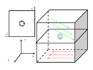
Figure 1: numerical setup: the sphere in the center of the box represent the area of the rotational perturbation. up-left is the rotational perturbation looked from YZ plane.

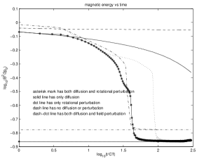
Figure 2: fast reconnection for different initial conditions

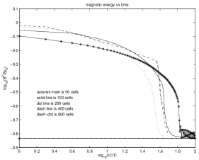
Figure 3: fast reconnection for different resolutions

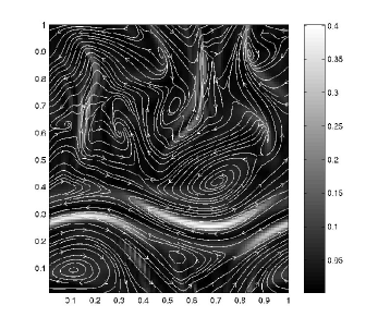
Figure 4: 2D snapshot during reconnection. current as background color

III Simulation results

III.1 Global fast magnetic reconnection

We use the total magnetic energy as a global diagnostic of the system. Figure 2 shows the evolution of the magnetic energy. The generic feature is the sudden drop of magnetic energy, which occurs on an alfvenic box crossing time, during which much of the magnetic energy is dissipated. The onset of this event depends on numerical parameters. Due to symmetries in the code, an absence of any initial perturbations would maintain the initial conditions indefinitely.

We can see that when there is no forced diffusion and no initial perturbation, the magnetic energy is almost stationary. When diffusion is added, the magnetic energy decays gradually throughout the simulation.

When explicit velocity perturbations are present, all the simulations show a sudden decrease of magnetic energy, which indicates fast magnetic reconnection. The common property is that they all have some initial perturbation, either rotational or a strong localized field perturbation; and the background diffusion only affects how early reconnection happens. In order to make sure this fast reconnection is not related to resolution, we simulate different resolutions, from a $50^{3}$ box, to a $800^{3}$ box, in Figure 3. All show fast reconnection and the resolution only affects the time elapsed before fast reconnection happens, though the details of how the delay depends on resolution are still unclear. Figure 4 shows a rough two dimensional snapshot of current($\propto\bigtriangledown\times{B}$) during fast reconnection, with color representing the current magnitude. It is clear that there are some regions that have reconnection(i.e. high current value) and we will use higher resolution to analyze them later. So, how fast is reconnection here? Since the magnetic energy is $\sim$ 50% at the onset of fast reconnection, the Alfven time is also $\sim$ CT and in the simulation, we find that nearly 50% of magnetic energy was released in one Alfven time during magnetic reconnection. This is clearly fast reconnection by any reasonable criteria.

III.2 What happens on the current sheet?

We can see there are some regions that have large currents, and the reconnection should happen there. Now we use high resolution (e.g. 800 cells) to investigate what exactly happens there. We want to show a snapshot close to the current sheet to see how flow evolves and what the magnetic field geometry looks like near the current sheet. We subtract the average value for both magnetic field and velocity in the region close to the current sheet. This places us in the frame comoving with the fluid. The mean magnetic field does not participate in the dynamics of reconnection, so its removal allows us to see the dynamics more clearly.

We present snapshots of three different times during the reconnection: one at the beginning, one at the middle and one at the end. Each time step snapshot contains three graphs, with the upper left one has current magnitude as background color and white line represents magnetic field line, and the lower left one is a snapshot of both magnetic field (blue dash) and velocity field (red solid), and the right one is the corresponding magnetic energy plot. Figure 6 is the beginning; Figure 7 is the middle; Figure 8 is the end;

It is easy to find that the snapshot of both magnetic field line and velocity field line in figure 6 looks like Figure 5 Petschek (1964), which is the geometry of Petschek’s solution for fast magnetic reconnection. The X-point, which is the reconnection region, is small and at the center. The tangent of the angle $\alpha$ represent the ratio of inflow to outflow.

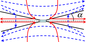
Figure 5: geometry of Petscheck solution

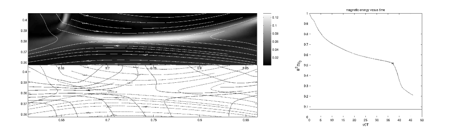
Figure 6: snapshot of magnetic field line on the background of current, and snapshot of both magnetic and velocity field line, and $B^{2}$ at 37 CT

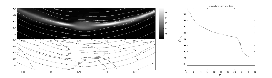
Figure 7: snapshot of magnetic field line on the background of current, and snapshot of both magnetic and velocity field line, and $B^{2}$ at 39 CT

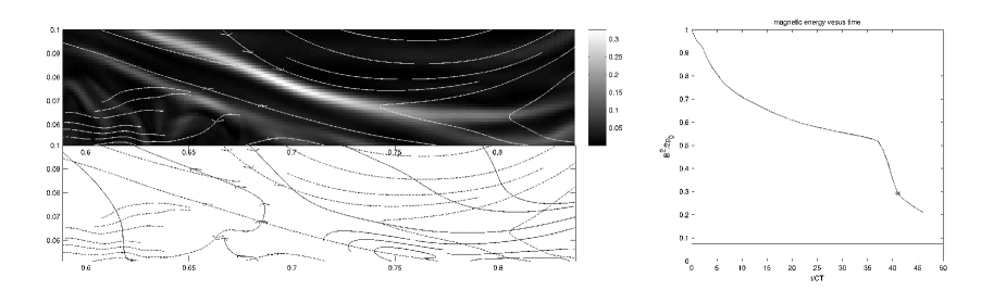
Figure 8: snapshot of magnetic field line on the background of current, and snapshot of both magnetic and velocity field line, and $B^{2}$ at 41 CT

III.3 What happens globally?

We show the long term and global 2D evolution of both velocity field lines and magnetic fields for the $400^{3}$ simulations, starting from the beginning until reconnection completes. These plots are analogous to the plots in the previous section: the left one is the snapshot of both magnetic and velocity field lines; the center one is the snapshot of magnetic field lines with current as the background color; and the corresponding magnetic energy is also included on the right. At the beginning, the magnetic field lines are opposite and there is no velocity field. Then the initial rotational perturbation induces two reconnected regions with closed magnetic field loops, one at each interface. The closed loops are fed by a slow X-point at each interface. Noting that there is a mean field perpendicular to the plotted surface, these loops are actually twists in the perpendicular magnetic field. In the bulk region between the interfaces, the parallel magnetic fields are not yet disturbed much by the perturbation.

In Figure 12 we can see the loops to move into the X-point of the opposing loop, and strong interactions occur. The fluid forms two large circular cells, offset from the magnetic loops. The energy to drive the fluid flow comes from the reconnection energy of the magnetic field. This flow pattern enhances the reconnection by driving the fluid through the X point. We illustrate the fast reconnection flows in Figure 9. Blue dash circles with arrows represent the magnetic loops. The red field lines with arrows represent the velocity field. There are two big black X’s in the global frame, which represent the X point for reconnection. Because we are using periodic boundary condition, we extend the simulation box picture to two other directions, to make the global flow easier to understand. Red solid lines represent the velocity field in the real box, and red dash-dot line represents the field line in the extended box.

Reconnection is a local process in the global flow field. To see that, we need to boost into the comoving frame. Let’s take the right magnetic twist for example: In global frame, the flow on the right all moves downwards, with the magnetic twist moving at the highest speed. The X-point is like a saddle point for the flow: the fluid converges vertically, and diverges horizontally. In the X-point frame, setting the velocity at B to zero, A will move down and C will move up, which supports the conditions for reconnection.

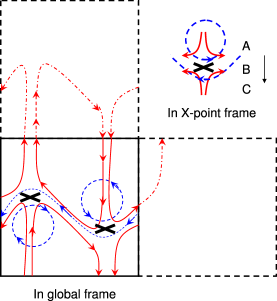
Figure 9: geometry of global configuration

Figure 10: snapshot of magnetic field line on the background of current, and snapshot of both magnetic and velocity field line, and $B^{2}$ at 0 CT for 400 cells

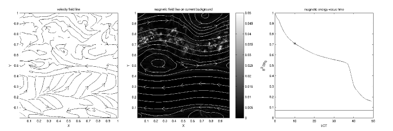
Figure 11: snapshot of magnetic field line on the background of current, and snapshot of both magnetic and velocity field line, and $B^{2}$ at 10 CT for 400 cells

Figure 12: snapshot of magnetic field line on the background of current, and snapshot of both magnetic and velocity field line, and $B^{2}$ at 38 CT for 400 cells

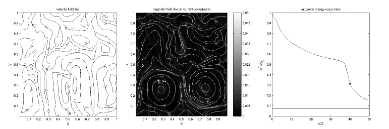
Figure 13: snapshot of magnetic field line on the background of current, and snapshot of both magnetic and velocity field line, and $B^{2}$ at 40 CT for 400 cells

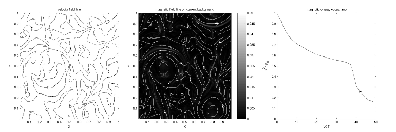
Figure 14: snapshot of magnetic field line on the background of current, and snapshot of both magnetic and velocity field line, and $B^{2}$ at 42 CT for 400 cells

IV Discussion

To summarize, we have found a global flow pattern which reinforces X-point reconnection, and the resulting fast reconnection in turn drives the global flow pattern. The basic picture is two dimensional. We did find that a pure 2-D simulation does not show this fast reconnection. This is easy to understand, since the reconnected field loops are loaded with matter, and would require resistivity to dissipate. In 3-D, these loops are twists which are unstable to a range of instabilities, allowing the field loops to collapse. So three basic ingredients are needed: 1. A global flow which keeps the field lines outside the X-point at a large opening angle to allow the reconnected fluid to escape, and avoid the Sweet-Parker time scale. 2. The reconnection energy drives this global flow 3. A three dimensional instability allows closed (reconnected) field lines to collapse, releasing all the energy stored in the field.

The problem described here has two geometric dimensionless parameters: the 2 axis ratios of the periodic box. In addition, there are a number of numerical parameters. We have varied them to study their effects.

Extending the box in the Y direction (separation between reconnection regions) shuts off this instability, which might be expected: there are no global flows possible if the two interaction regions are too far separated. We found the threshold to be $Y<1.2Z$. In the other direction, there appears to be no limit to make $Y<<Z$. Increasing the size of the Z dimension does not diminish this instability. There is also a dependence on X (extend along field symmetry axis). Shortening it to one grid cell protects the topology of field loops, and reconnection is not observed in 2-D simulations.

We changed different initial condition to see whether the fast reconnection is sensitive to how the initial setup is. After changing the angle of the opposite magnetic field(from beyond 90 degree to 180 degree), the strength of the rotational perturbation, and axis of the rotational perturbation, we found that the fast reconnection still appeared. The boundary condition is kept periodic and we found that the evolution of fluid dynamics of different initial conditions are similar.

It can be seen that the fast reconnection happens at the two interfaces of the straight magnetic field at the same time, with a magnetic twist moving towards it on each side. They are not head-on collision on the magnetic field, but a little separated in transverse direction. This special geometry helps the magnetic reconnection happen fast, since each magnetic twist pushes the field line, it also affect the velocity field at the other side and it helps to increase the outflow speed. If we look back to Sweet-Parker’s solution(Sweet (1958), Parker (1957)), the main problem is that the current sheet is so thin, that even if one accelerates the outflow to Alfven speed, the mass of outflow is still small, which slows down the speed of the reconnection. Petschek’s configurationPetschek (1964) can resolve this problem with a small reconnection region and finite opening angle for the outflow. In our simulation the speed of the outflow is further increased by the feedback between the two reconnection regions.

The solar flare reconnection time scale is about Alfven time scaleDere et al. (1991), which is the order of seconds to minutes.

If there is only magnetic diffusivity($\eta$) present, the diffusive time is $\tau_{D}=L^{2}/\eta$, with $L$ is the characteristic length. Taking the values from Dere et al. (1991), $L=1000km$ and $\eta$ is $10^{-3}{m^{2}}s^{-1}$, $\tau_{D}$ is $10^{15}s$.

Sweet-Parker’s thin current sheet proposed a reconnection time as $\tau_{SP}=L/(V_{Ai}/R_{mi}^{1/2})$, with $R_{mi}=L\upsilon_{Ai}/\eta$. This makes the reconnection time about $10^{5}$ Alfven times.

Petschek’s configuration has a reconnection time as $\tau_{P}=L/(\alpha\upsilon_{A})$, with $\alpha$ is between 0.01 and 0.1 and Alfven speed $\sim 100km/s$, and this makes the time scale as $100-1000s$.

Our fast reconnection time has the order of Alfven time scale, and Alfven time $\tau_{A}=L/\upsilon_{A}$, which is the same order as observed time scales of $20-60s$ Dere et al. (1991). Furthermore, comparing to LV99, no turbulence is needed or added in our simulations. Our fast magnetic reconnection time scale is qualitatively similar to the energy release time scale for solar flares.

V Summary

We present evidence for fast magnetic reconnection in a global three dimensional ideal magnetohydrodynamics simulation without any sustained external driving. These global simulations are self-contained, and do not rely on specified boundary conditions. We have quantified ranges in parameter space where fast reconnection is generic. The reconnection is Petscheck-like, and fast, meaning that nearly half of the magnetic energy is released in one Alfven time.

This example of fast reconnection example relies on two interacting reconnection regions in a periodic box. It is an intrinsically three dimensional effect. Our interpretation is that the Petschek-like X-point angles are not determined by microscopic properties at an infinitesimal boundary where no energy is present, but rather by the global flow far away from the X-point. Whether or not such configurations are natural in an open system remains to be seen.