Non-Sparse Regularization for Multiple Kernel Learning

Abstract

Learning linear combinations of multiple kernels is an appealing strategy when the right choice of features is unknown. Previous approaches to multiple kernel learning (MKL) promote sparse kernel combinations to support interpretability and scalability. Unfortunately, this $\ell_{1}$-norm MKL is rarely observed to outperform trivial baselines in practical applications. To allow for robust kernel mixtures, we generalize MKL to arbitrary norms. We devise new insights on the connection between several existing MKL formulations and develop two efficient interleaved optimization strategies for arbitrary norms, like $\ell_{p}$-norms with $p>1$. Empirically, we demonstrate that the interleaved optimization strategies are much faster compared to the commonly used wrapper approaches. A theoretical analysis and an experiment on controlled artificial data experiment sheds light on the appropriateness of sparse, non-sparse and $\ell_{\infty}$-norm MKL in various scenarios. Empirical applications of $\ell_{p}$-norm MKL to three real-world problems from computational biology show that non-sparse MKL achieves accuracies that go beyond the state-of-the-art.

Keywords: multiple kernel learning, learning kernels, non-sparse, support vector machine, convex conjugate, block coordinate descent, large scale optimization, bioinformatics, generalization bounds

1 Introduction

Kernels allow to decouple machine learning from data representations. Finding an appropriate data representation via a kernel function immediately opens the door to a vast world of powerful machine learning models (e.g. Schölkopf and Smola, 2002) with many efficient and reliable off-the-shelf implementations. This has propelled the dissemination of machine learning techniques to a wide range of diverse application domains.

Finding an appropriate data abstraction—or even engineering the best kernel—for the problem at hand is not always trivial, though. Starting with cross-validation (Stone, 1974), which is probably the most prominent approach to general model selection, a great many approaches to selecting the right kernel(s) have been deployed in the literature.

Kernel target alignment (Cristianini et al., 2002; Cortes et al., 2010b) aims at learning the entries of a kernel matrix by using the outer product of the label vector as the ground-truth. Chapelle et al. (2002) and Bousquet and Herrmann (2002) minimize estimates of the generalization error of support vector machines (SVMs) using a gradient descent algorithm over the set of parameters. Ong et al. (2005) study hyperkernels on the space of kernels and alternative approaches include selecting kernels by DC programming (Argyriou et al., 2008) and semi-infinite programming (Özögür-Akyüz and Weber, 2008; Gehler and Nowozin, 2008). Although finding non-linear kernel mixtures (Gönen and Alpaydin, 2008; Varma and Babu, 2009) generally results in non-convex optimization problems, Cortes et al. (2009b) show that convex relaxations may be obtained for special cases.

However, learning arbitrary kernel combinations is a problem too general to allow for a general optimal solution—by focusing on a restricted scenario, it is possible to achieve guaranteed optimality. In their seminal work, Lanckriet et al. (2004) consider training an SVM along with optimizing the linear combination of several positive semi-definite matrices, $K=\sum\nolimits_{m=1}^{M}\theta_{m}K_{m},$ subject to the trace constraint $\text{tr}(K)\leq c$ and requiring a valid combined kernel $K\succeq 0$. This spawned the new field of multiple kernel learning (MKL), the automatic combination of several kernel functions. Lanckriet et al. (2004) show that their specific version of the MKL task can be reduced to a convex optimization problem, namely a semi-definite programming (SDP) optimization problem. Though convex, however, the SDP approach is computationally too expensive for practical applications. Thus much of the subsequent research focuses on devising more efficient optimization procedures.

One conceptual milestone for developing MKL into a tool of practical utility is simply to constrain the mixing coefficients ${\boldsymbol{\theta}}$ to be non-negative: by obviating the complex constraint $K\succeq 0$, this small restriction allows one to transform the optimization problem into a quadratically constrained program, hence drastically reducing the computational burden. While the original MKL objective is stated and optimized in dual space, alternative formulations have been studied. For instance, Bach et al. (2004) found a corresponding primal problem, and Rubinstein (2005) decomposed the MKL problem into a min-max problem that can be optimized by mirror-prox algorithms (Nemirovski, 2004). The min-max formulation has been independently proposed by Sonnenburg et al. (2005). They use it to recast MKL training as a semi-infinite linear program. Solving the latter with column generation (e.g., Nash and Sofer, 1996) amounts to repeatedly training an SVM on a mixture kernel while iteratively refining the mixture coefficients ${\boldsymbol{\theta}}$. This immediately lends itself to a convenient implementation by a wrapper approach. These wrapper algorithms directly benefit from efficient SVM optimization routines (cf., e.g., Fan et al., 2005; Joachims, 1999) and are now commonly deployed in recent MKL solvers (e.g., Rakotomamonjy et al., 2008; Xu et al., 2009), thereby allowing for large-scale training (Sonnenburg et al., 2005, 2006a). However, the complete training of several SVMs can still be prohibitive for large data sets. For this reason, Sonnenburg et al. (2005) also propose to interleave the SILP with the SVM training which reduces the training time drastically. Alternative optimization schemes include level-set methods (Xu et al., 2009) and second order approaches (Chapelle and Rakotomamonjy, 2008). Szafranski et al. (2010), Nath et al. (2009), and Bach (2009) study composite and hierarchical kernel learning approaches. Finally, Zien and Ong (2007) and Ji et al. (2009) provide extensions for multi-class and multi-label settings, respectively.

Today, there exist two major families of multiple kernel learning models. The first is characterized by Ivanov regularization (Ivanov et al., 2002) over the mixing coefficients (Rakotomamonjy et al., 2007; Zien and Ong, 2007). For the Tikhonov-regularized optimization problem (Tikhonov and Arsenin, 1977), there is an additional parameter controlling the regularization of the mixing coefficients (Varma and Ray, 2007).

All the above mentioned multiple kernel learning formulations promote sparse solutions in terms of the mixing coefficients. The desire for sparse mixtures originates in practical as well as theoretical reasons. First, sparse combinations are easier to interpret. Second, irrelevant (and possibly expensive) kernels functions do not need to be evaluated at testing time. Finally, sparseness appears to be handy also from a technical point of view, as the additional simplex constraint $\|{\boldsymbol{\theta}}\|_{1}\leq 1$ simplifies derivations and turns the problem into a linearly constrained program. Nevertheless, sparseness is not always beneficial in practice and sparse MKL is frequently observed to be outperformed by a regular SVM using an unweighted-sum kernel $K=\sum_{m}K_{m}$ (Cortes et al., 2008).

Consequently, despite all the substantial progress in the field of MKL, there still remains an unsatisfied need for an approach that is really useful for practical applications: a model that has a good chance of improving the accuracy (over a plain sum kernel) together with an implementation that matches today’s standards (i.e., that can be trained on 10,000s of data points in a reasonable time). In addition, since the field has grown several competing MKL formulations, it seems timely to consolidate the set of models. In this article we argue that all of this is now achievable.

1.1 Outline of the Presented Achievements

On the theoretical side, we cast multiple kernel learning as a general regularized risk minimization problem for arbitrary convex loss functions, Hilbertian regularizers, and arbitrary norm-penalties on ${\boldsymbol{\theta}}$. We first show that the above mentioned Tikhonov and Ivanov regularized MKL variants are equivalent in the sense that they yield the same set of hypotheses. Then we derive a dual representation and show that a variety of methods are special cases of our objective. Our optimization problem subsumes state-of-the-art approaches to multiple kernel learning, covering sparse and non-sparse MKL by arbitrary $p$-norm regularization ($1\leq p\leq\infty$) on the mixing coefficients as well as the incorporation of prior knowledge by allowing for non-isotropic regularizers. As we demonstrate, the $p$-norm regularization includes both important special cases (sparse $1$-norm and plain sum $\infty$-norm) and offers the potential to elevate predictive accuracy over both of them.

With regard to the implementation, we introduce an appealing and efficient optimization strategy which grounds on an exact update in closed-form in the ${\boldsymbol{\theta}}$-step; hence rendering expensive semi-infinite and first- or second-order gradient methods unnecessary. By utilizing proven working set optimization for SVMs, $p$-norm MKL can now be trained highly efficiently for all $p$; in particular, we outpace other current $1$-norm MKL implementations. Moreover our implementation employs kernel caching techniques, which enables training on ten thousands of data points or thousands of kernels respectively. In contrast, most competing MKL software require all kernel matrices to be stored completely in memory, which restricts these methods to small data sets with limited numbers of kernels. Our implementation is freely available within the SHOGUN machine learning toolbox available at http://www.shogun-toolbox.org/.

Our claims are backed up by experiments on artificial data and on a couple of real world data sets representing diverse, relevant and challenging problems from the application domain bioinformatics. Experiments on artificial data enable us to investigate the relationship between properties of the true solution and the optimal choice of kernel mixture regularization. The real world problems include the prediction of the subcellular localization of proteins, the (transcription) starts of genes, and the function of enzymes. The results demonstrate (i) that combining kernels is now tractable on large data sets, (ii) that it can provide cutting edge classification accuracy, and (iii) that depending on the task at hand, different kernel mixture regularizations are required for achieving optimal performance.

In Appendix A we present a first theoretical analysis of non-sparse MKL. We introduce a novel $\ell_{1}$-to-$\ell_{p}$ conversion technique and use it to derive generalization bounds. Based on these, we perform a case study to compare a particular sparse with a non-sparse scenario.

A basic version of this work appeared in NIPS 2009 (Kloft et al., 2009a). The present article additionally offers a more general and complete derivation of the main optimization problem, exemplary applications thereof, a simple algorithm based on a closed-form solution, technical details of the implementation, a theoretical analysis, and additional experimental results. Parts of Appendix A are based on Kloft et al. (2010) the present analysis however extends the previous publication by a novel conversion technique, an illustrative case study, and an improved presentation.

Since its initial publication in Kloft et al. (2008), Cortes et al. (2009a), and Kloft et al. (2009a), non-sparse MKL has been subsequently applied, extended, and further analyzed by several researchers: Varma and Babu (2009) derive a projected gradient-based optimization method for $\ell_{2}$-norm MKL. Yu et al. (2010) present a more general dual view of $\ell_{2}$-norm MKL and show advantages of $\ell_{2}$-norm over an unweighted-sum kernel SVM on six bioinformatics data sets. Cortes et al. (2010a) provide generalization bounds for $\ell_{1}$- and $\ell_{p\leq 2}$-norm MKL. The analytical optimization method presented in this paper was independently and in parallel discovered by Xu et al. (2010) and has also been studied in Roth and Fischer (2007) and Ying et al. (2009) for $\ell_{1}$-norm MKL, and in Szafranski et al. (2010) and Nath et al. (2009) for composite kernel learning on small and medium scales.

The remainder is structured as follows. We derive non-sparse MKL in Section 2 and discuss relations to existing approaches in Section 3. Section 4 introduces the novel optimization strategy and its implementation. We report on our empirical results in Section 5. Section 6 concludes.

2 Multiple Kernel Learning – A Regularization View

In this section we cast multiple kernel learning into a unified framework: we present a regularized loss minimization formulation with additional norm constraints on the kernel mixing coefficients. We show that it comprises many popular MKL variants currently discussed in the literature, including seemingly different ones.

We derive generalized dual optimization problems without making specific assumptions on the norm regularizers or the loss function, beside that the latter is convex. Our formulation covers binary classification and regression tasks and can easily be extended to multi-class classification and structural learning settings using appropriate convex loss functions and joint kernel extensions. Prior knowledge on kernel mixtures and kernel asymmetries can be incorporated by non-isotropic norm regularizers.

2.1 Preliminaries

We begin with reviewing the classical supervised learning setup. Given a labeled sample $\mathcal{D}=\{(\boldsymbol{x}_{i},y_{i})\}_{i=1\ldots,n}$, where the $\boldsymbol{x}_{i}$ lie in some input space $\mathcal{X}$ and $y_{i}\in\mathcal{Y}\subset\mathbb{R}$, the goal is to find a hypothesis $h\in H$, that generalizes well on new and unseen data. Regularized risk minimization returns a minimizer $h^{*}$,

$$h^{*}\in\operatorname*{argmin}\nolimits_{h}\,\text{R}_{\text{emp}}(h)+\lambda\Omega(h),$$

where $\text{R}_{\text{emp}}(h)=\frac{1}{n}\sum_{i=1}^{n}V\left(h(\boldsymbol{x}_{i}),y_{i}\right)$ is the empirical risk of hypothesis $h$ w.r.t. a convex loss function $V:\mathbb{R}\times\mathcal{Y}\rightarrow\mathbb{R}$, $\Omega:H\rightarrow\mathbb{R}$ is a regularizer, and $\lambda>0$ is a trade-off parameter. We consider linear models of the form

$$h_{\tilde{\boldsymbol{w}},b}(\boldsymbol{x})=\langle\tilde{\boldsymbol{w}},\psi(\boldsymbol{x})\rangle+b,$$ (1)

together with a (possibly non-linear) mapping $\psi:\mathcal{X}\rightarrow\mathcal{H}$ to a Hilbert space $\mathcal{H}$ (e.g., Schölkopf et al., 1998; Müller et al., 2001) and constrain the regularization to be of the form $\Omega(h)=\frac{1}{2}\|\tilde{\boldsymbol{w}}\|_{2}^{2}$ which allows to kernelize the resulting models and algorithms. We will later make use of kernel functions $k(\boldsymbol{x},\boldsymbol{x}^{\prime})=\langle\psi(\boldsymbol{x}),\psi(\boldsymbol{x}^{\prime})\rangle_{\mathcal{H}}$ to compute inner products in $\mathcal{H}$.

2.2 Regularized Risk Minimization with Multiple Kernels

When learning with multiple kernels, we are given $M$ different feature mappings $\psi_{m}:\mathcal{X}\rightarrow\mathcal{H}_{m},~{}m=1,\ldots M$, each giving rise to a reproducing kernel $k_{m}$ of $\mathcal{H}_{m}$. Convex approaches to multiple kernel learning consider linear kernel mixtures $k_{\boldsymbol{\theta}}=\sum\theta_{m}k_{m}$, $\theta_{m}\geq 0$. Compared to Eq. (1), the primal model for learning with multiple kernels is extended to

$$h_{\tilde{\boldsymbol{w}},b,{\boldsymbol{\theta}}}(\boldsymbol{x})\,=\,\sum_{m=1}^{M}\sqrt{\theta_{m}}\langle\tilde{\boldsymbol{w}}_{m},\psi_{m}(\boldsymbol{x})\rangle_{\mathcal{H}_{m}}+b\,=\,\langle\tilde{\boldsymbol{w}},\psi_{{\boldsymbol{\theta}}}(\boldsymbol{x})\rangle_{\mathcal{H}}+b$$ (2)

where the parameter vector $\tilde{\boldsymbol{w}}$ and the composite feature map $\psi_{{\boldsymbol{\theta}}}$ have a block structure $\tilde{\boldsymbol{w}}=(\tilde{\boldsymbol{w}}_{1}^{\top},\ldots,\tilde{\boldsymbol{w}}^{\top}_{M})^{\top}$ and $\psi_{{\boldsymbol{\theta}}}=\sqrt{\theta_{1}}\psi_{1}\times\ldots\times\sqrt{\theta_{M}}\psi_{M}$, respectively.

In learning with multiple kernels we aim at minimizing the loss on the training data w.r.t. the optimal kernel mixture $\sum_{m=1}^{M}\theta_{m}k_{m}$ in addition to regularizing ${\boldsymbol{\theta}}$ to avoid overfitting. Hence, in terms of regularized risk minimization, the optimization problem becomes

$$\inf_{\tilde{\boldsymbol{w}},b,{\boldsymbol{\theta}}:{\boldsymbol{\theta}}\geq{\bf 0}}\quad\frac{1}{n}\sum_{i=1}^{n}V\left(\sum_{m=1}^{M}\sqrt{\theta_{m}}\langle\tilde{\boldsymbol{w}}_{m},\psi_{m}(\boldsymbol{x}_{i})\rangle_{\mathcal{H}_{m}}+b,~{}y_{i}\right)+\frac{\lambda}{2}\sum_{m=1}^{M}\|\tilde{w}_{m}\|_{\mathcal{H}_{m}}^{2}+\tilde{\mu}\tilde{\Omega}[{\boldsymbol{\theta}}],$$ (3)

for $\tilde{\mu}>0$. Note that the objective value of Eq. (3) is an upper bound on the training error. Previous approaches to multiple kernel learning employ regularizers of the form $\tilde{\Omega}({\boldsymbol{\theta}})=\|{\boldsymbol{\theta}}\|_{1}$ to promote sparse kernel mixtures. By contrast, we propose to use convex regularizers of the form $\tilde{\Omega}({\boldsymbol{\theta}})=\|{\boldsymbol{\theta}}\|^{2}$, where $\|\cdot\|^{2}$ is an arbitrary norm in $\mathbb{R}^{M}$, possibly allowing for non-sparse solutions and the incorporation of prior knowledge. The non-convexity arising from the $\sqrt{\theta_{m}}\tilde{\boldsymbol{w}}_{m}$ product in the loss term of Eq. (3) is not inherent and can be resolved by substituting $\boldsymbol{w}_{m}\leftarrow\sqrt{\theta_{m}}\tilde{\boldsymbol{w}}_{m}$. Furthermore, the regularization parameter and the sample size can be decoupled by introducing $\tilde{C}=\frac{1}{n\lambda}$ (and adjusting $\mu\leftarrow\frac{\tilde{\mu}}{\lambda}$) which has favorable scaling properties in practice. We obtain the following convex optimization problem (Boyd and Vandenberghe, 2004) that has also been considered by (Varma and Ray, 2007) for hinge loss and an $\ell_{1}$-norm regularizer

$$\inf_{\boldsymbol{w},b,{\boldsymbol{\theta}}:{\boldsymbol{\theta}}\geq{\bf 0}}\quad\tilde{C}\sum_{i=1}^{n}V\left(\sum_{m=1}^{M}\langle\boldsymbol{w}_{m},\psi_{m}(\boldsymbol{x}_{i})\rangle_{\mathcal{H}_{m}}+b,~{}y_{i}\right)+\frac{1}{2}\sum_{m=1}^{M}\frac{\|\boldsymbol{w}_{m}\|_{\mathcal{H}_{m}}^{2}}{\theta_{m}}+\mu\|{\boldsymbol{\theta}}\|^{2},$$ (4)

where we use the convention that $\frac{t}{0}=0$ if $t=0$ and $\infty$ otherwise.

An alternative approach has been studied by Rakotomamonjy et al. (2007) and Zien and Ong (2007), again using hinge loss and $\ell_{1}$-norm. They upper bound the value of the regularizer $\|{\boldsymbol{\theta}}\|_{1}\leq 1$ and incorporate the latter as an additional constraint into the optimization problem. For $C>0$, they arrive at the following problem which is the primary object of investigation in this paper.

Primal MKL Optimization Problem

$$\inf_{\boldsymbol{w},b,{\boldsymbol{\theta}}:{\boldsymbol{\theta}}\geq{\bf 0}}\quad C\sum_{i=1}^{n}V\Bigl{(}\sum_{m=1}^{M}\langle\boldsymbol{w}_{m},\psi_{m}(\boldsymbol{x}_{i})\rangle_{\mathcal{H}_{m}}+b,~{}y_{i}\Bigr{)}+\frac{1}{2}\sum_{m=1}^{M}\frac{\|\boldsymbol{w}_{m}\|_{\mathcal{H}_{m}}^{2}}{\theta_{m}}$$ (P)

s.t. $$\|{\boldsymbol{\theta}}\|^{2}\leq 1.$$

It is important to note here that, while the Ivanov regularization in (4) has two regularization parameters ($C$ and $\mu$), the above Tikhonov regularization (P) has only one ($C$ only). Our first contribution shows that, despite the additional regularization parameter, both MKL variants are equivalent, in the sense that traversing the regularization paths yields the same binary classification functions.

Theorem 1.

Let $\|\cdot\|$ be a norm on $\mathbb{R}^{M}$, be $V$ a convex loss function. Suppose for the optimal $\boldsymbol{w}^{*}$ in Optimization Problem (P) it holds $\boldsymbol{w}^{*}\neq\mathbf{0}$. Then, for each pair $(\tilde{C},\mu)$ there exists $C>0$ such that for each optimal solution ($\boldsymbol{w},b,\theta$) of Eq. (4) using $(\tilde{C},\mu)$, we have that $(\boldsymbol{w},b,\kappa\,{\boldsymbol{\theta}})$ is also an optimal solution of Optimization Problem (P) using ${C}$, and vice versa, where $\kappa>0$ is a multiplicative constant.

For the proof we need Prop. 11, which justifies switching from Ivanov to Tikhonov regularization, and back, if the regularizer is tight. We refer to Appendix B for the proposition and its proof.

Proof.

of Theorem 1 Let be $(\tilde{C},\mu)>0$. In order to apply Prop. 11 to (4), we show that condition (37) in Prop. 11 is satisfied, i.e., that the regularizer is tight.

Suppose on the contrary, that Optimization Problem (P) yields the same infimum regardless of whether we require

$$\|{\boldsymbol{\theta}}\|^{2}\leq 1,$$ (5)

or not. Then this implies that in the optimal point we have $\sum_{m=1}^{M}\frac{\|\boldsymbol{w}^{*}_{m}\|_{2}^{2}}{\theta^{*}_{m}}=0$, hence,

$$\frac{\|\boldsymbol{w}^{*}_{m}\|_{2}^{2}}{\theta^{*}_{m}}=0,~{}~{}\forall~{}m=1,\ldots,M.$$ (6)

Since all norms on $\mathbb{R}^{M}$ are equivalent (e.g., Rudin, 1991), there exists a $L<\infty$ such that $\|{\boldsymbol{\theta}}^{*}\|_{\infty}\leq L\|{\boldsymbol{\theta}}^{*}\|$. In particular, we have $\|{\boldsymbol{\theta}}^{*}\|_{\infty}<\infty$, from which we conclude by (6), that $\boldsymbol{w}_{m}=0$ holds for all $m$, which contradicts our assumption.

Hence, Prop. 11 can be applied, which yields that (4) is equivalent to

$$\inf_{\boldsymbol{w},b,{\boldsymbol{\theta}}}\quad \tilde{C}\sum_{i=1}^{n}V\Bigl{(}\sum_{m=1}^{M}\langle\boldsymbol{w}_{m},\psi_{m}(\boldsymbol{x})\rangle+b,~{}y_{i}\Bigr{)}+\frac{1}{2}\sum_{m=1}^{M}\frac{\|\boldsymbol{w}_{m}\|_{2}^{2}}{\theta_{m}}$$

s.t. $$\|{\boldsymbol{\theta}}\|^{2}\leq\tau,$$

for some $\tau>0$. Consider the optimal solution $(\boldsymbol{w}^{\star},b^{\star},{\boldsymbol{\theta}}^{\star})$ corresponding to a given parametrization $(\tilde{C},\tau)$. For any $\lambda>0$, the bijective transformation $(\tilde{C},\tau)\mapsto(\lambda^{-1/2}\tilde{C},\lambda\tau)$ will yield $(\boldsymbol{w}^{\star},b^{\star},\lambda^{1/2}{\boldsymbol{\theta}}^{\star})$ as optimal solution. Applying the transformation with $\lambda:=1/\tau$ and setting $C=\tilde{C}\tau^{\frac{1}{2}}$ as well as $\kappa=\tau^{-1/2}$ yields Optimization Problem (P), which was to be shown. ∎

Zien and Ong (2007) also show that the MKL optimization problems by Bach et al. (2004), Sonnenburg et al. (2006a), and their own formulation are equivalent. As a main implication of Theorem 1 and by using the result of Zien and Ong it follows that the optimization problem of Varma and Ray (Varma and Ray, 2007) lies in the same equivalence class as (Bach et al., 2004; Sonnenburg et al., 2006a; Rakotomamonjy et al., 2007; Zien and Ong, 2007). In addition, our result shows the coupling between trade-off parameter $C$ and the regularization parameter $\mu$ in Eq. (4): tweaking one also changes the other and vice versa. Theorem 1 implies that optimizing $C$ in Optimization Problem (P) implicitly searches the regularization path for the parameter $\mu$ of Eq. (4). In the remainder, we will therefore focus on the formulation in Optimization Problem (P), as a single parameter is preferable in terms of model selection.

2.3 MKL in Dual Space

In this section we study the generalized MKL approach of the previous section in the dual space. Let us begin with rewriting Optimization Problem (P) by expanding the decision values into slack variables as follows

$$\inf_{\boldsymbol{w},b,\boldsymbol{t},{\boldsymbol{\theta}}:{\boldsymbol{\theta}}\geq{\bf 0}} \quad C\sum_{i=1}^{n}V\left(t_{i},~{}y_{i}\right)+\frac{1}{2}\sum_{m=1}^{M}\frac{\|\boldsymbol{w}_{m}\|_{\mathcal{H}_{m}}^{2}}{\theta_{m}}$$ (7)

s.t. $$\quad\forall i:~{}\sum_{m=1}^{M}\langle\boldsymbol{w}_{m},\psi_{m}(\boldsymbol{x}_{i})\rangle_{\mathcal{H}_{m}}+b=t_{i}~{};\quad\|{\boldsymbol{\theta}}\|^{2}\leq 1,$$

where $\|\cdot\|$ is an arbitrary norm in $\mathbb{R}^{m}$ and $\|\cdot\|_{\mathcal{H}_{M}}$ denotes the Hilbertian norm of $\mathcal{H}_{m}$. Applying Lagrange’s theorem re-incorporates the constraints into the objective by introducing Lagrangian multipliers ${\boldsymbol{\alpha}}\in\mathbb{R}^{n}$ and $\beta\in\mathbb{R}_{+}$. The Lagrangian saddle point problem is then given by

$$\sup_{{\boldsymbol{\alpha}},\beta:\beta\geq 0}~{}\inf_{\boldsymbol{w},b,\boldsymbol{t},{\boldsymbol{\theta}}\geq 0}\quad C\sum_{i=1}^{n}V\left(t_{i},~{}y_{i}\right)+\frac{1}{2}\sum_{m=1}^{M}\frac{\|\boldsymbol{w}_{m}\|_{\mathcal{H}_{m}}^{2}}{\theta_{m}}$$ (8)

$$-\sum_{i=1}^{n}\alpha_{i}\left(\sum_{m=1}^{M}\langle\boldsymbol{w}_{m},\psi_{m}(\boldsymbol{x}_{i})\rangle_{\mathcal{H}_{m}}+b-t_{i}\right)+\beta\left(\frac{1}{2}\|{\boldsymbol{\theta}}\|^{2}-\frac{1}{2}\right).$$

Denoting the Lagrangian by $\mathcal{L}$ and setting its first partial derivatives with respect to $\boldsymbol{w}$ and $b$ to $0$ reveals the optimality conditions

$$\mathbf{1}^{\top}{\boldsymbol{\alpha}}=0;$$ (9a)

$$\boldsymbol{w}_{m}=\theta_{m}\sum_{i=1}^{n}\alpha_{i}\psi_{m}(\boldsymbol{x}_{i}),~{}~{}\forall\hskip 2.84526ptm=1,\ldots,M.$$ (9b)

Resubstituting the above equations yields

$$\sup_{{\boldsymbol{\alpha}}:~{}\mathbf{1}^{\top}{\boldsymbol{\alpha}}=0,~{}\beta:\beta\geq 0}~{}\inf_{\boldsymbol{t},{\boldsymbol{\theta}}\geq 0}\quad C\sum_{i=1}^{n}\left(V\left(t_{i},~{}y_{i}\right)+\alpha_{i}t_{i}\right)-\frac{1}{2}\sum_{m=1}^{M}\theta_{m}{\boldsymbol{\alpha}}^{\top}K_{m}{\boldsymbol{\alpha}}+\beta\left(\frac{1}{2}\|{\boldsymbol{\theta}}\|^{2}-\frac{1}{2}\right),$$

which can also be written in terms of unconstrained ${\boldsymbol{\theta}}$, because the supremum with respect to ${\boldsymbol{\theta}}$ is attained for non-negative ${\boldsymbol{\theta}}\geq 0$. We arrive at

$$\sup_{{\boldsymbol{\alpha}}:~{}\mathbf{1}^{\top}{\boldsymbol{\alpha}}=0,~{}\beta\geq 0}-C\sum_{i=1}^{n}\sup_{t_{i}}\left(-\frac{\alpha_{i}}{C}t_{i}-V\left(t_{i},~{}y_{i}\right)\right)-\beta\sup_{{\boldsymbol{\theta}}}\left(\frac{1}{2\beta}\sum_{m=1}^{M}\theta_{m}{\boldsymbol{\alpha}}^{\top}K_{m}{\boldsymbol{\alpha}}-\frac{1}{2}\|{\boldsymbol{\theta}}\|^{2}\right)-\frac{1}{2}\beta.$$

As a consequence, we now may express the Lagrangian as

$$\sup_{{\boldsymbol{\alpha}}:~{}\mathbf{1}^{\top}{\boldsymbol{\alpha}}=0,~{}\beta\geq 0}~{}-C\sum_{i=1}^{n}V^{*}\left(-\frac{\alpha_{i}}{C},~{}y_{i}\right)-\frac{1}{2\beta}\left\|\frac{1}{2}\left({\boldsymbol{\alpha}}^{\top}K_{m}{\boldsymbol{\alpha}}\right)_{m=1}^{M}\right\|^{2}_{*}-\frac{1}{2}\beta,$$ (10)

where $h^{*}(\boldsymbol{x})=\sup_{\boldsymbol{u}}\boldsymbol{x}^{\top}\boldsymbol{u}-h(\boldsymbol{u})$ denotes the Fenchel-Legendre conjugate of a function $h$ and $\|\cdot\|_{*}$ denotes the dual norm, i.e., the norm defined via the identity $\frac{1}{2}\|\cdot\|^{2}_{*}:=\left(\frac{1}{2}\|\cdot\|^{2}\right)^{*}$. In the following, we call $V^{*}$ the dual loss. Eq. (10) now has to be maximized with respect to the dual variables ${\boldsymbol{\alpha}},\beta$, subject to $\mathbf{1}^{\top}{\boldsymbol{\alpha}}=0$ and $\beta\geq 0$. Let us ignore for a moment the non-negativity constraint on $\beta$ and solve $\partial\mathcal{L}/\partial{\beta}=0$ for the unbounded $\beta$. Setting the partial derivative to zero allows to express the optimal $\beta$ as

$$\beta=\left\|\frac{1}{2}\left({\boldsymbol{\alpha}}^{\top}K_{m}{\boldsymbol{\alpha}}\right)_{m=1}^{M}\right\|_{*}.$$ (11)

Obviously, at optimality, we always have $\beta\geq 0$. We thus discard the corresponding constraint from the optimization problem and plugging Eq. (11) into Eq. (10) results in the following dual optimization problem which now solely depends on ${\boldsymbol{\alpha}}$:

Dual MKL Optimization Problem

$$\sup_{{\boldsymbol{\alpha}}:~{}\mathbf{1}^{\top}{\boldsymbol{\alpha}}=0}~{}-C\sum_{i=1}^{n}V^{*}\left(-\frac{\alpha_{i}}{C},~{}y_{i}\right)-\frac{1}{2}\left\|\left({\boldsymbol{\alpha}}^{\top}K_{m}{\boldsymbol{\alpha}}\right)_{m=1}^{M}\right\|_{*}.$$ (D)

The above dual generalizes multiple kernel learning to arbitrary convex loss functions and norms. Note that if the loss function is continuous (e.g., hinge loss), the supremum is also a maximum. The threshold $b$ can be recovered from the solution by applying the KKT conditions.

The above dual can be characterized as follows. We start by noting that the expression in Optimization Problem (D) is a composition of two terms, first, the left hand side term, which depends on the conjugate loss function $V^{*}$, and, second, the right hand side term which depends on the conjugate norm. The right hand side can be interpreted as a regularizer on the quadratic terms that, according to the chosen norm, smoothens the solutions. Hence we have a decomposition of the dual into a loss term (in terms of the dual loss) and a regularizer (in terms of the dual norm). For a specific choice of a pair $(V,\|\cdot\|)$ we can immediately recover the corresponding dual by computing the pair of conjugates $(V^{*},\|\cdot\|_{*})$ (for a comprehensive list of dual losses see Rifkin and Lippert, 2007, Table 3). In the next section, this is illustrated by means of well-known loss functions and regularizers.

At this point we would like to highlight some properties of Optimization Problem (D) that arise due to our dualization technique. While approaches that firstly apply the representer theorem and secondly optimize in the primal such as Chapelle (2006) also can employ general loss functions, the resulting loss terms depend on all optimization variables. By contrast, in our formulation the dual loss terms are of a much simpler structure and they only depend on a single optimization variable $\alpha_{i}$. A similar dualization technique yielding singly-valued dual loss terms is presented in Rifkin and Lippert (2007); it is based on Fenchel duality and limited to strictly positive definite kernel matrices. Our technique, which uses Lagrangian duality, extends the latter by allowing for positive semi-definite kernel matrices.

3 Instantiations of the Model

In this section we show that existing MKL-based learners are subsumed by the generalized formulation in Optimization Problem (D).

3.1 Support Vector Machines with Unweighted-Sum Kernels

First we note that the support vector machine with an unweighted-sum kernel can be recovered as a special case of our model. To see this, we consider the regularized risk minimization problem using the hinge loss function $V(t,y)=\max(0,1-ty)$ and the regularizer $\|\theta\|_{\infty}$. We then can obtain the corresponding dual in terms of Fenchel-Legendre conjugate functions as follows.

We first note that the dual loss of the hinge loss is $V^{*}(t,y)=\frac{t}{y}$ if $-1\leq\frac{t}{y}\leq 0$ and $\infty$ elsewise (Rifkin and Lippert, 2007, Table 3). Hence, for each $i$ the term $V^{*}\left(-\frac{\alpha_{i}}{C},~{}y_{i}\right)$ of the generalized dual, i.e., Optimization Problem (D), translates to $-\frac{\alpha_{i}}{Cy_{i}}$, provided that $0\leq\frac{\alpha_{i}}{y_{i}}\leq C$. Employing a variable substitution of the form $\alpha^{\text{new}}_{i}=\frac{\alpha_{i}}{y_{i}}$, Optimization Problem (D) translates to

$$\max_{\boldsymbol{\alpha}}~{}~{}\mathbf{1}^{\top}{\boldsymbol{\alpha}}-\frac{1}{2}\left\|\left({\boldsymbol{\alpha}}^{\top}YK_{m}Y{\boldsymbol{\alpha}}\right)_{m=1}^{M}\right\|_{*},\quad\text{s.t.}\quad{\boldsymbol{y}^{\top}{\boldsymbol{\alpha}}=0~{}~{}\text{and}~{}~{}\mathbf{0}\leq{\boldsymbol{\alpha}}\leq C\mathbf{1}},$$ (12)

where we denote $Y={\rm diag}(y)$. The primal $\ell_{\infty}$-norm penalty $\|{\boldsymbol{\theta}}\|_{\infty}$ is dual to $\|{\boldsymbol{\theta}}\|_{1}$, hence, via the identity $\|\cdot\|_{*}=\|\cdot\|_{1}$ the right hand side of the last equation translates to $\sum_{m=1}^{M}{\boldsymbol{\alpha}}^{\top}YK_{m}Y{\boldsymbol{\alpha}}$. Combined with (12) this leads to the dual

$$\sup_{\boldsymbol{\alpha}}~{}~{}\mathbf{1}^{\top}{\boldsymbol{\alpha}}-\frac{1}{2}\sum_{m=1}^{M}{\boldsymbol{\alpha}}^{\top}YK_{m}Y{\boldsymbol{\alpha}},\quad\text{s.t.}\quad{\boldsymbol{y}^{\top}{\boldsymbol{\alpha}}=0~{}~{}\text{and}~{}~{}\mathbf{0}\leq{\boldsymbol{\alpha}}\leq C\mathbf{1}},$$

which is precisely an SVM with an unweighted-sum kernel.

3.2 QCQP MKL of Lanckriet et al. (2004)

A common approach in multiple kernel learning is to employ regularizers of the form

$$\Omega({\boldsymbol{\theta}})=\|{\boldsymbol{\theta}}\|_{1}.$$ (13)

This so-called $\ell_{1}$-norm regularizers are specific instances of sparsity-inducing regularizers. The obtained kernel mixtures usually have a considerably large fraction of zero entries, and hence equip the MKL problem by the favor of interpretable solutions. Sparse MKL is a special case of our framework; to see this, note that the conjugate of (13) is $\|\cdot\|_{\infty}$. Recalling the definition of an $\ell_{p}$-norm, the right hand side of Optimization Problem (D) translates to $\max_{m\in\{1,\ldots,M\}}{\boldsymbol{\alpha}}^{\top}YK_{m}Y{\boldsymbol{\alpha}}$. The maximum can subsequently be expanded into a slack variable $\xi$, resulting in

$$\sup_{{\boldsymbol{\alpha}},\boldsymbol{\xi}} \quad\mathbf{1}^{\top}{\boldsymbol{\alpha}}-\xi$$

s.t. $$\quad\forall\hskip 2.84526ptm:\;\;\frac{1}{2}{\boldsymbol{\alpha}}^{\top}YK_{m}Y{\boldsymbol{\alpha}}\leq\xi~{};\quad\boldsymbol{y}^{\top}{\boldsymbol{\alpha}}=0~{};\quad\mathbf{0}\leq{\boldsymbol{\alpha}}\leq C\mathbf{1},$$

which is the original QCQP formulation of MKL, firstly given by Lanckriet et al. (2004).

3.3 $\ell_{p}$-Norm MKL

Our MKL formulation also allows for robust kernel mixtures by employing an $\ell_{p}$-norm constraint with $p>1$, rather than an $\ell_{1}$-norm constraint, on the mixing coefficients (Kloft et al., 2009a). The following identity holds

$$\left(\frac{1}{2}\|\cdot\|_{p}^{2}\right)^{*}=\frac{1}{2}\|\cdot\|^{2}_{p^{*}},$$

where $p^{*}:=\frac{p}{p-1}$ is the conjugated exponent of $p$, and we obtain for the dual norm of the $\ell_{p}$-norm: $\|\cdot\|_{*}=\|\cdot\|_{p^{*}}$. This leads to the dual problem

$$\sup_{{\boldsymbol{\alpha}}:\mathbf{1}^{\top}{\boldsymbol{\alpha}}=\mathbf{0}}~{}-C\sum_{i=1}^{n}V^{*}\left(-\frac{\alpha_{i}}{C},~{}y_{i}\right)-\frac{1}{2}\left\|\left({\boldsymbol{\alpha}}^{\top}K_{m}{\boldsymbol{\alpha}}\right)_{m=1}^{M}\right\|_{p^{*}}.$$

In the special case of hinge loss minimization, we obtain the optimization problem

$$\sup_{\boldsymbol{\alpha}}~{}~{}\mathbf{1}^{\top}{\boldsymbol{\alpha}}-\frac{1}{2}\left\|\left({\boldsymbol{\alpha}}^{\top}YK_{m}Y{\boldsymbol{\alpha}}\right)_{m=1}^{M}\right\|_{p^{*}},\quad\text{s.t.}\quad{\boldsymbol{y}^{\top}{\boldsymbol{\alpha}}=0~{}~{}\text{and}~{}~{}\mathbf{0}\leq{\boldsymbol{\alpha}}\leq C\mathbf{1}}.$$

3.4 A Smooth Variant of Group Lasso

Yuan and Lin (2006) studied the following optimization problem for the special case $\mathcal{H}_{m}=\mathbb{R}^{d_{m}}$ and $\psi_{m}={\rm id}_{\mathbb{R}^{d_{m}}}$, also known as group lasso,

$$\min_{\boldsymbol{w}}\quad\frac{C}{2}\sum_{i=1}^{n}\left(y_{i}-\sum_{m=1}^{M}\langle\boldsymbol{w}_{m},\psi_{m}(\boldsymbol{x}_{i})\rangle_{\mathcal{H}_{m}}\right)^{2}+\frac{1}{2}\sum_{m=1}^{M}\|\boldsymbol{w}_{m}\|_{\mathcal{H}_{m}}.$$ (14)

The above problem has been solved by active set methods in the primal (Roth and Fischer, 2008). We sketch an alternative approach based on dual optimization. First, we note that Eq. (14) can be equivalently expressed as (Micchelli and Pontil, 2005, Lemma 26)

$$\inf_{\boldsymbol{w},{\boldsymbol{\theta}}:{\boldsymbol{\theta}}\geq{\bf 0}}\quad\frac{C}{2}\sum_{i=1}^{n}\left(y_{i}-\sum_{m=1}^{M}\langle\boldsymbol{w}_{m},\psi_{m}(\boldsymbol{x}_{i})\rangle_{\mathcal{H}_{m}}\right)^{2}+\frac{1}{2}\sum_{m=1}^{M}\frac{\|\boldsymbol{w}_{m}\|_{\mathcal{H}_{m}}^{2}}{\theta_{m}},\quad\text{s.t.}\quad\|{\boldsymbol{\theta}}\|^{2}_{1}\leq 1.$$

The dual of $V(t,y)=\frac{1}{2}(y-t)^{2}$ is $V^{*}(t,y)=\frac{1}{2}t^{2}+ty$ and thus the corresponding group lasso dual can be written as

$$\max_{\boldsymbol{\alpha}}\quad\boldsymbol{y}^{\top}{\boldsymbol{\alpha}}-\frac{1}{2C}\|{\boldsymbol{\alpha}}\|_{2}^{2}-\frac{1}{2}\left\|\left({\boldsymbol{\alpha}}^{\top}YK_{m}Y{\boldsymbol{\alpha}}\right)_{m=1}^{M}\right\|_{\infty},$$ (15)

which can be expanded into the following QCQP

$$\sup_{{\boldsymbol{\alpha}},\xi} \quad\boldsymbol{y}^{\top}{\boldsymbol{\alpha}}-\frac{1}{2C}\|{\boldsymbol{\alpha}}\|_{2}^{2}-{\color[rgb]{0,0,0}\xi}$$ (16)

s.t. $$\quad\forall\hskip 0.85358ptm:\quad\frac{1}{2}{\boldsymbol{\alpha}}^{\top}YK_{m}Y{\boldsymbol{\alpha}}\leq{\color[rgb]{0,0,0}\xi}.$$

For small $n$, the latter formulation can be handled efficiently by QCQP solvers. However, the quadratic constraints caused by the non-smooth $\ell_{\infty}$-norm in the objective still are computationally too demanding. As a remedy, we propose the following unconstrained variant based on $\ell_{p}$-norms ($1<p<\infty$), given by

$$\max_{\boldsymbol{\alpha}}\quad\boldsymbol{y}^{\top}{\boldsymbol{\alpha}}-\frac{1}{2C}\|{\boldsymbol{\alpha}}\|_{2}^{2}-\frac{1}{2}\left\|\left({\boldsymbol{\alpha}}^{\top}YK_{m}Y{\boldsymbol{\alpha}}\right)_{m=1}^{M}\right\|_{p^{*}}.$$

It is straight forward to verify that the above objective function is differentiable in any ${\boldsymbol{\alpha}}\in\mathbb{R}^{n}$ (in particular, notice that the $\ell_{p}$-norm function is differentiable for $1<p<\infty$) and hence the above optimization problem can be solved very efficiently by, for example, limited memory quasi-Newton descent methods (Liu and Nocedal, 1989).

3.5 Density Level-Set Estimation

Density level-set estimators are frequently used for anomaly/novelty detection tasks (Markou and Singh, 2003a, b). Kernel approaches, such as one-class SVMs (Schölkopf et al., 2001) and Support Vector Domain Descriptions (Tax and Duin, 1999) can be cast into our MKL framework by employing loss functions of the form $V(t)=\max(0,1-t)$. This gives rise to the primal

$$\inf_{\boldsymbol{w},{\boldsymbol{\theta}}:{\boldsymbol{\theta}}\geq{\bf 0}}\quad C\sum_{i=1}^{n}\max\left(0,\sum_{m=1}^{M}\langle\boldsymbol{w}_{m},\psi_{m}(\boldsymbol{x}_{i})\rangle_{\mathcal{H}_{m}}\right)+\frac{1}{2}\sum_{m=1}^{M}\frac{\|\boldsymbol{w}_{m}\|_{\mathcal{H}_{m}}^{2}}{\theta_{m}},\quad\text{s.t.}\quad\|{\boldsymbol{\theta}}\|^{2}\leq 1.$$

Noting that the dual loss is $V^{*}(t)=t$ if $-1\leq t\leq 0$ and $\infty$ elsewise, we obtain the following generalized dual

$$\sup_{{\boldsymbol{\alpha}}}~{}~{}\mathbf{1}^{\top}{\boldsymbol{\alpha}}-\frac{1}{2}\left\|\left({\boldsymbol{\alpha}}^{\top}K_{m}{\boldsymbol{\alpha}}\right)_{m=1}^{M}\right\|_{p^{*}},\quad\text{s.t.}\quad{\mathbf{0}\leq{\boldsymbol{\alpha}}\leq C\mathbf{1}},$$

which has been studied by Sonnenburg et al. (2006a) and Rakotomamonjy et al. (2008) for $\ell_{1}$-norm, and by Kloft et al. (2009b) for $\ell_{p}$-norms.

3.6 Non-Isotropic Norms

In practice, it is often desirable for an expert to incorporate prior knowledge about the problem domain. For instance, an expert could provide estimates of the interactions of kernels $\{K_{1},...,K_{M}\}$ in the form of an $M\times M$ matrix $E$. Alternatively, $E$ could be obtained by computing pairwise kernel alignments $E_{ij}=\frac{<K_{i},K_{j}>}{\|K_{i}\|~{}\|K_{j}\|}$ given a dot product on the space of kernels such as the Frobenius dot product (Ong et al., 2005). In a third scenario, $E$ could be a diagonal matrix encoding the a priori importance of kernels—it might be known from pilot studies that a subset of the employed kernels is inferior to the remaining ones.

All those scenarios can be easily handled within our framework by considering non-isotropic regularizers of the form

$$\|{\boldsymbol{\theta}}\|_{E^{-1}}=\sqrt{{\boldsymbol{\theta}}^{\top}E^{-1}{\boldsymbol{\theta}}}~{}~{}\text{with}~{}~{}E\succ 0,$$

where $E^{-1}$ is the matrix inverse of $E$. The dual norm is again defined via $\frac{1}{2}\|\cdot\|^{2}_{*}:=\left(\frac{1}{2}\|\cdot\|^{2}_{E^{-1}}\right)^{*}$ and the following easily-to-verify identity,

$$\left(\frac{1}{2}\|\cdot\|^{2}_{E^{-1}}\right)^{*}=\frac{1}{2}\|\cdot\|_{E}^{2},$$

leads to the dual,

$$\sup_{{\boldsymbol{\alpha}}:\mathbf{1}^{\top}{\boldsymbol{\alpha}}=\mathbf{0}}~{}-C\sum_{i=1}^{n}V^{*}\left(-\frac{\alpha_{i}}{C},~{}y_{i}\right)-\frac{1}{2}\left\|\left({\boldsymbol{\alpha}}^{\top}K_{m}{\boldsymbol{\alpha}}\right)_{m=1}^{M}\right\|_{E},$$

which is the desired non-isotropic MKL problem.

4 Optimization Strategies

The dual as given in Optimization Problem (D) does not lend itself to efficient large-scale optimization in a straight-forward fashion, for instance by direct application of standard approaches like gradient descent. Instead, it is beneficial to exploit the structure of the MKL cost function by alternating between optimizing w.r.t. the mixings ${\boldsymbol{\theta}}$ and w.r.t. the remaining variables. Most recent MKL solvers (e.g., Rakotomamonjy et al., 2008; Xu et al., 2009; Nath et al., 2009) do so by setting up a two-layer optimization procedure: a master problem, which is parameterized only by ${\boldsymbol{\theta}}$, is solved to determine the kernel mixture; to solve this master problem, repeatedly a slave problem is solved which amounts to training a standard SVM on a mixture kernel. Importantly, for the slave problem, the mixture coefficients are fixed, such that conventional, efficient SVM optimizers can be recycled. Consequently these two-layer procedures are commonly implemented as wrapper approaches. Albeit appearing advantageous, wrapper methods suffer from two shortcomings: (i) Due to kernel cache limitations, the kernel matrices have to be pre-computed and stored or many kernel computations have to be carried out repeatedly, inducing heavy wastage of either memory or time. (ii) The slave problem is always optimized to the end (and many convergence proofs seem to require this), although most of the computational time is spend on the non-optimal mixtures. Certainly suboptimal slave solutions would already suffice to improve far-from-optimal ${\boldsymbol{\theta}}$ in the master problem.

Due to these problems, MKL is prohibitive when learning with a multitude of kernels and on large-scale data sets as commonly encountered in many data-intense real world applications such as bioinformatics, web mining, databases, and computer security. The optimization approach presented in this paper decomposes the MKL problem into smaller subproblems (Platt, 1999; Joachims, 1999; Fan et al., 2005) by establishing a wrapper-like scheme within the decomposition algorithm.

Our algorithm is embedded into the large-scale framework of Sonnenburg et al. (2006a) and extends it to the optimization of non-sparse kernel mixtures induced by an $\ell_{p}$-norm penalty. Our strategy alternates between minimizing the primal problem (7) w.r.t. ${\boldsymbol{\theta}}$ via a simple analytical update formula and with incomplete optimization w.r.t. all other variables which, however, is performed in terms of the dual variables ${\boldsymbol{\alpha}}$. Optimization w.r.t. ${\boldsymbol{\alpha}}$ is performed by chunking optimizations with minor iterations. Convergence of our algorithm is proven under typical technical regularity assumptions.

4.1 A Simple Wrapper Approach Based on an Analytical Update

We first present an easy-to-implement wrapper version of our optimization approach to multiple kernel learning. The interleaved decomposition algorithm is deferred to the next section. To derive the new algorithm, we first revisit the primal problem, i.e.

$$\inf_{\boldsymbol{w},b,{\boldsymbol{\theta}}:{\boldsymbol{\theta}}\geq{\bf 0}}\quad C\sum_{i=1}^{n}V\left(\sum_{m=1}^{M}\langle\boldsymbol{w}_{m},\psi_{m}(\boldsymbol{x}_{i})\rangle_{\mathcal{H}_{m}}+b,~{}y_{i}\right)+\frac{1}{2}\sum_{m=1}^{M}\frac{\|\boldsymbol{w}_{m}\|_{\mathcal{H}_{m}}^{2}}{\theta_{m}},\quad\text{s.t.}\quad\|{\boldsymbol{\theta}}\|^{2}\leq 1.~{}~{}~{}(P)$$

In order to obtain an efficient optimization strategy, we divide the variables in the above OP into two groups, $(\boldsymbol{w},b)$ on one hand and ${\boldsymbol{\theta}}$ on the other. In the following we will derive an algorithm which alternatingly operates on those two groups via a block coordinate descent algorithm, also known as the non-linear block Gauss-Seidel method. Thereby the optimization w.r.t. ${\boldsymbol{\theta}}$ will be carried out analytically and the $(\boldsymbol{w},b)$-step will be computed in the dual, if needed.

The basic idea of our first approach is that for a given, fixed set of primal variables $(\boldsymbol{w},b)$, the optimal ${\boldsymbol{\theta}}$ in the primal problem (P) can be calculated analytically. In the subsequent derivations we employ non-sparse norms of the form $\|{\boldsymbol{\theta}}\|_{p}=(\sum_{m=1}^{M}\theta_{m}^{p})^{{1}/{p}}$, $1<p<\infty$.

The following proposition gives an analytic update formula for ${\boldsymbol{\theta}}$ given fixed remaining variables $(\boldsymbol{w},b)$ and will become the core of our proposed algorithm.

Proposition 2.

Let $V$ be a convex loss function, be $p>1$. Given fixed (possibly suboptimal) $\boldsymbol{w}\neq\mathbf{0}$ and $b$, the minimal ${\boldsymbol{\theta}}$ in Optimization Problem (P) is attained for

$$\theta_{m}=\frac{\|\boldsymbol{w}_{m}\|_{\mathcal{H}_{m}}^{\frac{2}{p+1}}}{\left(\sum_{m^{\prime}=1}^{M}\|\boldsymbol{w}_{m^{\prime}}\|_{\mathcal{H}_{m^{\prime}}}^{\frac{2p}{p+1}}\right)^{{1}/{p}}},\quad~{}\forall m=1,\ldots,M.$$ (17)

Proof.

We start the derivation, by equivalently translating Optimization Problem (P) via Theorem 1 into

$$\inf_{\boldsymbol{w},b,{\boldsymbol{\theta}}:{\boldsymbol{\theta}}\geq{\bf 0}}\quad\tilde{C}\sum_{i=1}^{n}V\left(\sum_{m=1}^{M}\langle\boldsymbol{w}_{m},\psi_{m}(\boldsymbol{x}_{i})\rangle_{\mathcal{H}_{m}}+b,~{}y_{i}\right)+\frac{1}{2}\sum_{m=1}^{M}\frac{\|\boldsymbol{w}_{m}\|_{\mathcal{H}_{m}}^{2}}{\theta_{m}}+\frac{\mu}{2}\|{\boldsymbol{\theta}}\|_{p}^{2},$$ (18)

with $\mu>0$. Suppose we are given fixed $(\boldsymbol{w},b)$, then setting the partial derivatives of the above objective w.r.t. ${\boldsymbol{\theta}}$ to zero yields the following condition on the optimality of ${\boldsymbol{\theta}}$,

$$-\frac{\|\boldsymbol{w}_{m}\|_{\mathcal{H}_{m}}^{2}}{2\theta_{m}^{2}}+\mu\cdot\frac{\partial\left(\frac{1}{2}\|{\boldsymbol{\theta}}\|_{p}^{2}\right)}{\partial\theta_{m}}=0,\quad\forall m=1,\ldots,M.$$ (19)

The first derivative of the $\ell_{p}$-norm with respect to the mixing coefficients can be expressed as

$$\frac{\partial\left(\frac{1}{2}\|{\boldsymbol{\theta}}\|_{p}^{2}\right)}{\partial\theta_{m}}=\theta_{m}^{p-1}\|{\boldsymbol{\theta}}\|_{p}^{2-p},$$

and hence Eq. (19) translates into the following optimality condition,

$$\exists\zeta\quad\forall m=1,\ldots,M:~{}~{}\quad\theta_{m}=\zeta\|\boldsymbol{w}_{m}\|_{\mathcal{H}_{m}}^{\frac{2}{p+1}}~{}.\quad\quad$$ (20)

Because $\boldsymbol{w}\neq 0$, using the same argument as in the proof of Theorem 1, the constraint $\|{\boldsymbol{\theta}}\|^{2}_{p}\leq 1$ in (18) is at the upper bound, i.e.  $\|{\boldsymbol{\theta}}\|_{p}=1$ holds for an optimal ${\boldsymbol{\theta}}$. Inserting (20) in the latter equation leads to $\zeta=\left(\sum_{m=1}^{M}\|\boldsymbol{w}_{m}\|_{\mathcal{H}_{m}}^{{2p}/{p+1}}\right)^{{1}/{p}}$. Resubstitution into (20) yields the claimed formula (17). ∎

Second, we consider how to optimize Optimization Problem (P) w.r.t. the remaining variables $(\boldsymbol{w},b)$ for a given set of mixing coefficients ${\boldsymbol{\theta}}$. Since optimization often is considerably easier in the dual space, we fix ${\boldsymbol{\theta}}$ and build the partial Lagrangian of Optimization Problem (P) w.r.t. all other primal variables $\boldsymbol{w}$, $b$. The resulting dual problem is of the form (detailed derivations omitted)

$$\sup_{{\boldsymbol{\alpha}}:\mathbf{1}^{\top}{\boldsymbol{\alpha}}=0} -C\sum_{i=1}^{n}V^{*}\left(-\frac{\alpha_{i}}{C},~{}y_{i}\right)-\frac{1}{2}\sum_{m=1}^{M}\theta_{m}{\boldsymbol{\alpha}}^{\top}K_{m}{\boldsymbol{\alpha}},$$ (21)

and the KKT conditions yield $\boldsymbol{w}_{m}=\theta_{m}\sum_{i=1}^{n}\alpha_{i}\psi_{m}(\boldsymbol{x}_{i})$ in the optimal point, hence

$$\|\boldsymbol{w}_{m}\|^{2}=\theta_{m}^{2}{\boldsymbol{\alpha}}K_{m}{\boldsymbol{\alpha}},\quad\forall~{}m=1,\ldots,M.$$ (22)

We now have all ingredients (i.e., Eqs. (17), (21)–(22)) to formulate a simple macro-wrapper algorithm for $\ell_{p}$-norm MKL training:

1:  input: feasible ${\boldsymbol{\alpha}}$ and ${\boldsymbol{\theta}}$

2:  while optimality conditions are not satisfied do

3:    Compute ${\boldsymbol{\alpha}}$ according to Eq. (21) (e.g. SVM)

4:    Compute $\|\boldsymbol{w}_{m}\|^{2}$ for all $m=1,...,M$ according to Eq. (22)

5:    Update ${\boldsymbol{\theta}}$ according to Eq. (17)

6:  end while

Algorithm 1 Simple $\ell_{p>1}$-norm MKL wrapper-based training algorithm. The analytical updates of ${\boldsymbol{\theta}}$ and the SVM computations are optimized alternatingly.

The above algorithm alternatingly solves a convex risk minimization machine (e.g. SVM) w.r.t. the actual mixture ${\boldsymbol{\theta}}$ (Eq. (21)) and subsequently computes the analytical update according to Eq. (17) and (22). It can, for example, be stopped based on changes of the objective function or the duality gap within subsequent iterations.

4.2 Towards Large-Scale MKL—Interleaving SVM and MKL Optimization

However, a disadvantage of the above wrapper approach still is that it deploys a full blown kernel matrix. We thus propose to interleave the SVM optimization of SVMlight with the ${\boldsymbol{\theta}}$- and ${\boldsymbol{\alpha}}$-steps at training time. We have implemented this so-called interleaved algorithm in Shogun for hinge loss, thereby promoting sparse solutions in $\alpha$. This allows us to solely operate on a small number of active variables. The resulting interleaved optimization method is shown in Algorithm 2. Lines 3-5 are standard in chunking based SVM solvers and carried out by $\text{SVM}^{\text{light}}$ (note that $Q$ is chosen as described in Joachims (1999)). Lines 6-7 compute SVM-objective values. Finally, the analytical ${\boldsymbol{\theta}}$-step is carried out in Line 9. The algorithm terminates if the maximal KKT violation (c.f. Joachims, 1999) falls below a predetermined precision $\varepsilon$ and if the normalized maximal constraint violation $|1-\frac{\omega}{\omega_{\text{o}ld}}|<\varepsilon_{mkl}$ for the MKL-step, where $\omega$ denotes the MKL objective function value (Line 8).

1:  Initialize: $g_{m,i}=\hat{g}_{i}=\alpha_{i}=0$, $\forall i=1,...,n$;  $L=S=-\infty$;  $\theta_{m}=\sqrt[p]{1/M}$, $\forall m=1,...,M$

2:  iterate

3:   Select Q variables $\alpha_{i_{1}},\ldots,\alpha_{i_{Q}}$ based on the gradient $\hat{\bf g}$ of (21) w.r.t. ${\boldsymbol{\alpha}}$

4:   Store ${\boldsymbol{\alpha}}^{old}={\boldsymbol{\alpha}}$ and then update ${\boldsymbol{\alpha}}$ according to (21) with respect to the selected variables

5:   Update gradient $g_{m,i}\leftarrow g_{m,i}+\sum_{q=1}^{Q}(\alpha_{i_{q}}-\alpha^{old}_{i_{q}})k_{m}(\boldsymbol{x}_{i_{q}},\boldsymbol{x}_{i})$,  $\forall$ $m=1,\ldots,M$, $i=1,\ldots,n$

6:   Compute the quadratic terms  $S_{m}=\frac{1}{2}\sum_{i}g_{m,i}\alpha_{i}$,  $q_{m}=2\theta_{m}^{2}S_{m}$, $~{}\forall m=1,\ldots,M$

7:   $L_{\text{o}ld}=L$,  $L=\sum_{i}y_{i}\alpha_{i}$,  $S_{\text{o}ld}=S$,  $S=\sum_{m}\theta_{m}S_{m}$

8:   if $|1-\frac{L-S}{L_{\text{o}ld}-S_{\text{o}ld}}|\geq\varepsilon$

9:    $\theta_{m}=\left(q_{m}\right)^{1/(p+1)}/\left(\sum_{m^{\prime}=1}^{M}\left(q_{m^{\prime}}\right)^{p/(p+1)}\right)^{1/p},\quad\forall~{}m=1,\ldots,M$

10:   else

11:    break

12:   end if

13:   $\hat{g}_{i}=\sum_{m}\theta_{m}g_{m,i}$ for all $i=1,\ldots,n$

Algorithm 2   $\ell_{p}$-Norm MKL chunking-based training algorithm via analytical update. Kernel weighting ${\boldsymbol{\theta}}$ and (signed) SVM ${\boldsymbol{\alpha}}$ are optimized interleavingly. The accuracy parameter $\varepsilon$ and the subproblem size $Q$ are assumed to be given to the algorithm.

4.3 Convergence Proof for $p>1$

In the following, we exploit the primal view of the above algorithm as a nonlinear block Gauss-Seidel method, to prove convergence of our algorithms. We first need the following useful result about convergence of the nonlinear block Gauss-Seidel method in general.

Proposition 3 (Bertsekas, 1999, Prop. 2.7.1).

Let $\mathcal{X}=\bigotimes_{m=1}^{M}\mathcal{X}_{m}$ be the Cartesian product of closed convex sets $\mathcal{X}_{m}\subset\mathbb{R}^{d_{m}}$, be $f:\mathcal{X}\rightarrow\mathbb{R}$ a continuously differentiable function. Define the nonlinear block Gauss-Seidel method recursively by letting $\boldsymbol{x}^{0}\in\mathcal{X}$ be any feasible point, and be

$$\boldsymbol{x}_{m}^{k+1}=\operatorname*{argmin}_{\boldsymbol{\xi}\in\mathcal{X}_{m}}f\left(\boldsymbol{x}_{1}^{k+1},\cdots,\boldsymbol{x}_{m-1}^{k+1},\boldsymbol{\xi},\boldsymbol{x}_{m+1}^{k},\cdots,\boldsymbol{x}_{M}^{k}\right),~{}~{}\forall m=1,\ldots,M.$$ (23)

Suppose that for each $m$ and $\boldsymbol{x}\in\mathcal{X}$, the minimum

$$\min_{\boldsymbol{\xi}\in\mathcal{X}_{m}}f\left(\boldsymbol{x}_{1},\cdots,\boldsymbol{x}_{m-1},\boldsymbol{\xi},\boldsymbol{x}_{m+1},\cdots,\boldsymbol{x}_{M}\right)$$ (24)

is uniquely attained. Then every limit point of the sequence $\{\boldsymbol{x}^{k}\}_{k\in\mathbb{N}}$ is a stationary point.

The proof can be found in Bertsekas (1999), p. 268-269. The next proposition basically establishes convergence of the proposed $\ell_{p}$-norm MKL training algorithm.

Theorem 4.

Let $V$ be the hinge loss and be $p>1$. Let the kernel matrices $K_{1},\ldots,K_{M}$ be positive definite. Then every limit point of Algorithm 1 is a globally optimal point of Optimization Problem (P). Moreover, suppose that the SVM computation is solved exactly in each iteration, then the same holds true for Algorithm 2.

Proof.

If we ignore the numerical speed-ups, then the Algorithms 1 and 2 coincidence for the hinge loss. Hence, it suffices to show the wrapper algorithm converges.

To this aim, we have to transform Optimization Problem (P) into a form such that the requirements for application of Prop. 3 are fulfilled. We start by expanding Optimization Problem (P) into

$$\min_{\boldsymbol{w},b,{\boldsymbol{\xi}},{\boldsymbol{\theta}}} \quad C\sum_{i=1}^{n}\xi_{i}+\frac{1}{2}\sum_{m=1}^{M}\frac{\|\boldsymbol{w}_{m}\|_{\mathcal{H}_{m}}^{2}}{\theta_{m}},$$

s.t. $$\quad\forall i:~{}\sum_{m=1}^{M}\langle\boldsymbol{w}_{m},\psi_{m}(\boldsymbol{x}_{i})\rangle_{\mathcal{H}_{m}}+b\geq 1-\xi_{i};\quad{\boldsymbol{\xi}}\geq 0;\quad\|{\boldsymbol{\theta}}\|_{p}^{2}\leq 1;\quad{\boldsymbol{\theta}}\geq{\bf 0},$$

thereby extending the second block of variables, $(\boldsymbol{w},b)$, into $(\boldsymbol{w},b,{\boldsymbol{\xi}})$. Moreover, we note that after an application of the representer theorem (Kimeldorf and Wahba, 1971) we may without loss of generality assume $\mathcal{H}_{m}=\mathbb{R}^{n}$.

In the problem’s current form, the possibility of $\theta_{m}=0$ while $\boldsymbol{w}_{m}\neq 0$ renders the objective function nondifferentiable. This hinders the application of Prop. 3. Fortunately, it follows from Prop. 2 (note that $K_{m}\succ 0$ implies $\boldsymbol{w}\neq\mathbf{0}$) that this case is impossible. We therefore can substitute the constraint ${\boldsymbol{\theta}}\geq\mathbf{0}$ by ${\boldsymbol{\theta}}>\mathbf{0}$ for all $m$. In order to maintain the closeness of the feasible set we subsequently apply a bijective coordinate transformation $\phi:\mathbb{R}^{M}_{+}\rightarrow\mathbb{R}^{M}$ with $\theta_{m}^{\text{new}}=\phi_{m}(\theta_{m})=\log(\theta_{m})$, resulting in the following equivalent problem,

$$\inf_{\boldsymbol{w},b,{\boldsymbol{\xi}},{\boldsymbol{\theta}}} \quad C\sum_{i=1}^{n}\xi_{i}+\frac{1}{2}\sum_{m=1}^{M}\exp(-\theta_{m})\|\boldsymbol{w}_{m}\|_{\mathbb{R}^{n}}^{2},$$

s.t. $$\quad\forall i:~{}\sum_{m=1}^{M}\langle\boldsymbol{w}_{m},\psi_{m}(\boldsymbol{x}_{i})\rangle_{\mathbb{R}^{n}}+b\geq 1-\xi_{i};\quad{\boldsymbol{\xi}}\geq 0;\quad\|\exp({\boldsymbol{\theta}})\|_{p}^{2}\leq 1,$$

where we employ the notation $\exp({\boldsymbol{\theta}})=\left(\exp(\theta_{1}),\cdots,\exp(\theta_{M})\right)^{\top}$.

Applying the Gauss-Seidel method in Eq. (23) to the base problem (P) and to the reparametrized problem yields the same sequence of solutions $\{(\boldsymbol{w},b,{\boldsymbol{\theta}})^{k}\}_{k\in\mathbb{N}_{0}}$. The above problem now allows to apply Prop. 3 for the two blocks of coordinates ${\boldsymbol{\theta}}\in\mathcal{X}_{1}$ and $(\boldsymbol{w},b,{\boldsymbol{\xi}})\in\mathcal{X}_{2}$: the objective is continuously differentiable and the sets $\mathcal{X}_{1}$ are closed and convex. To see the latter, note that $\|\cdot\|_{p}^{2}\circ\exp$ is a convex function, since $\|\cdot\|_{p}^{2}$ is convex and non-increasing in each argument (cf., e.g., Section 3.2.4 in Boyd and Vandenberghe, 2004). Moreover, the minima in Eq. (23) are uniquely attained: the $(\boldsymbol{w},b)$-step amounts to solving an SVM on a positive definite kernel mixture, and the analytical ${\boldsymbol{\theta}}$-step clearly yields unique solutions as well.

Hence, we conclude that every limit point of the sequence $\{(\boldsymbol{w},b,{\boldsymbol{\theta}})^{k}\}_{k\in\mathbb{N}}$ is a stationary point of Optimization Problem (P). For a convex problem, this is equivalent to such a limit point being globally optimal. ∎

In practice, we are facing two problems. First, the standard Hilbert space setup necessarily implies that $\left\|\boldsymbol{w}_{m}\right\|\geq 0$ for all $m$. However in practice this assumption may often be violated, either due to numerical imprecision or because of using an indefinite “kernel” function. However, for any $\left\|\boldsymbol{w}_{m}\right\|\leq 0$ it also follows that $\theta^{\star}_{m}=0$ as long as at least one strictly positive $\left\|\boldsymbol{w}_{m^{\prime}}\right\|>0$ exists. This is because for any $\lambda<0$ we have $\lim_{h\rightarrow 0,h>0}\frac{\lambda}{h}=-\infty$. Thus, for any $m$ with $\left\|\boldsymbol{w}_{m}\right\|\leq 0$, we can immediately set the corresponding mixing coefficients $\theta^{\star}_{m}$ to zero. The remaining ${\boldsymbol{\theta}}$ are then computed according to Equation (2), and convergence will be achieved as long as at least one strictly positive $\left\|\boldsymbol{w}_{m^{\prime}}\right\|>0$ exists in each iteration.

Second, in practice, the SVM problem will only be solved with finite precision, which may lead to convergence problems. Moreover, we actually want to improve the ${\boldsymbol{\alpha}}$ only a little bit before recomputing ${\boldsymbol{\theta}}$ since computing a high precision solution can be wasteful, as indicated by the superior performance of the interleaved algorithms (cf. Sect. 5.5). This helps to avoid spending a lot of ${\boldsymbol{\alpha}}$-optimization (SVM training) on a suboptimal mixture ${\boldsymbol{\theta}}$. Fortunately, we can overcome the potential convergence problem by ensuring that the primal objective decreases within each ${\boldsymbol{\alpha}}$-step. This is enforced in practice, by computing the SVM by a higher precision if needed. However, in our computational experiments we find that this precaution is not even necessary: even without it, the algorithm converges in all cases that we tried (cf. Section 5).

Finally, we would like to point out that the proposed block coordinate descent approach lends itself more naturally to combination with primal SVM optimizers like (Chapelle, 2006), LibLinear (Fan et al., 2008) or Ocas (Franc and Sonnenburg, 2008). Especially for linear kernels this is extremely appealing.

4.4 Technical Considerations

4.4.1 Implementation Details

We have implemented the analytic optimization algorithm described in the previous Section, as well as the cutting plane and Newton algorithms by Kloft et al. (2009a), within the SHOGUN toolbox (Sonnenburg et al., 2010) for regression, one-class classification, and two-class classification tasks. In addition one can choose the optimization scheme, i.e., decide whether the interleaved optimization algorithm or the wrapper algorithm should be applied. In all approaches any of the SVMs contained in SHOGUN can be used. Our implementation can be downloaded from http://www.shogun-toolbox.org.

In the more conventional family of approaches, the wrapper algorithms, an optimization scheme on ${\boldsymbol{\theta}}$ wraps around a single kernel SVM. Effectively this results in alternatingly solving for ${\boldsymbol{\alpha}}$ and ${\boldsymbol{\theta}}$. For the outer optimization (i.e., that on ${\boldsymbol{\theta}}$) SHOGUN offers the three choices listed above. The semi-infinite program (SIP) uses a traditional SVM to generate new violated constraints and thus requires a single kernel SVM. A linear program (for $p=1$) or a sequence of quadratically constrained linear programs (for $p>1$) is solved via GLPK or IBM ILOG CPLEX. Alternatively, either an analytic or a Newton update (for $\ell_{p}$ norms with $p>1$) step can be performed, obviating the need for an additional mathematical programming software.

The second, much faster approach performs interleaved optimization and thus requires modification of the core SVM optimization algorithm. It is currently integrated into the chunking-based SVRlight and SVMlight. To reduce the implementation effort, we implement a single function perform_mkl_step($\sum_{{\boldsymbol{\alpha}}}$, obj_m), that has the arguments $\sum_{{\boldsymbol{\alpha}}}=\sum_{i=1}^{n}\alpha_{i}$ and obj_m=$\frac{1}{2}{\boldsymbol{\alpha}}^{T}K_{m}{\boldsymbol{\alpha}}$, i.e. the current linear ${\boldsymbol{\alpha}}$-term and the SVM objectives for each kernel. This function is either, in the interleaved optimization case, called as a callback function (after each chunking step or a couple of SMO steps), or it is called by the wrapper algorithm (after each SVM optimization to full precision).

Recovering Regression and One-Class Classification.

It should be noted that one-class classification is trivially implemented using $\sum_{{\boldsymbol{\alpha}}}=0$ while support vector regression (SVR) is typically performed by internally translating the SVR problem into a standard SVM classification problem with twice the number of examples once positively and once negatively labeled with corresponding ${\boldsymbol{\alpha}}$ and ${\boldsymbol{\alpha}}^{*}$. Thus one needs direct access to ${\boldsymbol{\alpha}}^{*}$ and computes $\sum_{{\boldsymbol{\alpha}}}=-\sum_{i=1}^{n}(\alpha_{i}+\alpha_{i}^{*})\varepsilon-\sum_{i=1}^{n}(\alpha_{i}-\alpha_{i}^{*})y_{i}$ (cf. Sonnenburg et al., 2006a). Since this requires modification of the core SVM solver we implemented SVR only for interleaved optimization and SVMlight.

Efficiency Considerations and Kernel Caching.

Note that the choice of the size of the kernel cache becomes crucial when applying MKL to large scale learning applications. While for the wrapper algorithms only a single kernel SVM needs to be solved and thus a single large kernel cache should be used, the story is different for interleaved optimization. Since one must keep track of the several partial MKL objectives obj_m, requiring access to individual kernel rows, the same cache size should be used for all sub-kernels.

4.4.2 Kernel Normalization

The normalization of kernels is as important for MKL as the normalization of features is for training regularized linear or single-kernel models. This is owed to the bias introduced by the regularization: optimal feature / kernel weights are requested to be small. This is easier to achieve for features (or entire feature spaces, as implied by kernels) that are scaled to be of large magnitude, while downscaling them would require a correspondingly upscaled weight for representing the same predictive model. Upscaling (downscaling) features is thus equivalent to modifying regularizers such that they penalize those features less (more). As is common practice, we here use isotropic regularizers, which penalize all dimensions uniformly. This implies that the kernels have to be normalized in a sensible way in order to represent an “uninformative prior” as to which kernels are useful.

There exist several approaches to kernel normalization, of which we use two in the computational experiments below. They are fundamentally different. The first one generalizes the common practice of standardizing features to entire kernels, thereby directly implementing the spirit of the discussion above. In contrast, the second normalization approach rescales the data points to unit norm in feature space. Nevertheless it can have a beneficial effect on the scaling of kernels, as we argue below.

Multiplicative Normalization.

As done in Ong and Zien (2008), we multiplicatively normalize the kernels to have uniform variance of data points in feature space. Formally, we find a positive rescaling $\rho_{m}$ of the kernel, such that the rescaled kernel $\tilde{k}_{m}(\cdot,\cdot)=\rho_{m}k_{m}(\cdot,\cdot)$ and the corresponding feature map $\tilde{\Phi}_{m}(\cdot)=\sqrt{\rho_{m}}\Phi_{m}(\cdot)$ satisfy

$$\frac{1}{n}\sum_{i=1}^{n}\left\|\tilde{\Phi}_{m}(\boldsymbol{x}_{i})-\tilde{\Phi}_{m}(\bar{\boldsymbol{x}})\right\|^{2}=1$$

for each $m=1,\ldots,M$, where $\tilde{\Phi}_{m}(\bar{\boldsymbol{x}}):=\frac{1}{n}\sum_{i=1}^{n}\tilde{\Phi}_{m}(\boldsymbol{x}_{i})$ is the empirical mean of the data in feature space. The above equation can be equivalently be expressed in terms of kernel functions as

$$\frac{1}{n}\sum_{i=1}^{n}\tilde{k}_{m}(\boldsymbol{x}_{i},\boldsymbol{x}_{i})-\frac{1}{n^{2}}\sum_{i=1}^{n}\sum_{j=1}^{n}\tilde{k}_{m}(\boldsymbol{x}_{i},\boldsymbol{x}_{j})=1,$$

so that the final normalization rule is

$$k(\boldsymbol{x},\bar{\boldsymbol{x}})\longmapsto\frac{k(\boldsymbol{x},\bar{\boldsymbol{x}})}{\frac{1}{n}\sum_{i=1}^{n}k(\boldsymbol{x}_{i},\boldsymbol{x}_{i})-\frac{1}{n^{2}}\sum_{i,j=1}^{n},k(\boldsymbol{x}_{i},\boldsymbol{x}_{j})}.$$ (25)

Note that in case the kernel is centered (i.e. the empirical mean of the data points lies on the origin), the above rule simplifies to $k(\boldsymbol{x},\bar{\boldsymbol{x}})\longmapsto{k(\boldsymbol{x},\bar{\boldsymbol{x}})}/{\frac{1}{n}{\rm tr}(K)}$, where ${\rm tr}(K):=\sum_{i=1}^{n}k(\boldsymbol{x}_{i},\boldsymbol{x}_{i})$ is the trace of the kernel matrix $K$.

Spherical Normalization.

Frequently, kernels are normalized according to

$$k(\boldsymbol{x},\bar{\boldsymbol{x}})\longmapsto\frac{k(\boldsymbol{x},\bar{\boldsymbol{x}})}{\sqrt{k(\boldsymbol{x},\boldsymbol{x})k(\bar{\boldsymbol{x}},\bar{\boldsymbol{x}})}}.$$ (26)

After this operation, $\|\boldsymbol{x}\|=k(\boldsymbol{x},\boldsymbol{x})=1$ holds for each data point $x$; this means that each data point is rescaled to lie on the unit sphere. Still, this also may have an effect on the scale of the features: a spherically normalized and centered kernel is also always multiplicatively normalized, because the multiplicative normalization rule becomes $k(\boldsymbol{x},\bar{\boldsymbol{x}})\longmapsto{k(\boldsymbol{x},\bar{\boldsymbol{x}})}/{\frac{1}{n}{\rm tr}(K)}={k(\boldsymbol{x},\bar{\boldsymbol{x}})}/1$.

Thus the spherical normalization may be seen as an approximation to the above multiplicative normalization and may be used as a substitute for it. Note, however, that it changes the data points themselves by eliminating length information; whether this is desired or not depends on the learning task at hand. Finally note that both normalizations achieve that the optimal value of $C$ is not far from $1$.

4.5 Limitations and Extensions of our Framework

In this section, we show the connection of $\ell_{p}$-norm MKL to a formulation based on block norms, point out limitations and sketch extensions of our framework. To this aim let us recall the primal MKL problem (P) and consider the special case of $\ell_{p}$-norm MKL given by

$$\inf_{\boldsymbol{w},b,{\boldsymbol{\theta}}:{\boldsymbol{\theta}}\geq{\bf 0}}\quad C\sum_{i=1}^{n}V\left(\sum_{m=1}^{M}\langle\boldsymbol{w}_{m},\psi_{m}(\boldsymbol{x}_{i})\rangle_{\mathcal{H}_{m}}+b,~{}y_{i}\right)+\frac{1}{2}\sum_{m=1}^{M}\frac{\|\boldsymbol{w}_{m}\|_{\mathcal{H}_{m}}^{2}}{\theta_{m}},\quad\text{s.t.}\quad\|{\boldsymbol{\theta}}\|_{p}^{2}\leq 1.$$ (27)

The subsequent proposition shows that (27) equivalently can be translated into the following mixed-norm formulation,

$$\inf_{\boldsymbol{w},b}\quad\tilde{C}\sum_{i=1}^{n}V\left(\sum_{m=1}^{M}\langle\boldsymbol{w}_{m},\psi_{m}(\boldsymbol{x}_{i})\rangle_{\mathcal{H}_{m}}+b,~{}y_{i}\right)+\frac{1}{2}\sum_{m=1}^{M}\|\boldsymbol{w}_{m}\|_{\mathcal{H}_{m}}^{q},$$ (28)

where $q=\frac{2p}{p+1}$, and $\tilde{C}$ is a constant. This has been studied by Bach et al. (2004) for $q=1$ and by Szafranski et al. (2008) for hierarchical penalization.

Proposition 5.

Let be $p>1$, be $V$ a convex loss function, and define $q:=\frac{2p}{p+1}$ (i.e. $p=\frac{q}{2-q}$). Optimization Problem (27) and (28) are equivalent, i.e., for each $C$ there exists a $\tilde{C}>0$, such that for each optimal solution ($\boldsymbol{w}^{*},b^{*},\theta^{*}$) of OP (27) using $C$, we have that ($\boldsymbol{w}^{*},b^{*}$) is also optimal in OP (28) using $\tilde{C}$, and vice versa.

Proof.

From Prop. 2 it follows that for any fixed $\boldsymbol{w}$ in (27) it holds for the $\boldsymbol{w}$-optimal ${\boldsymbol{\theta}}$:

$$\exists\zeta:~{}~{}\theta_{m}=\zeta\|\boldsymbol{w}_{m}\|_{\mathcal{H}_{m}}^{\frac{2}{p+1}},\quad\forall m=1,\ldots,M.$$

Plugging the above equation into (27) yields

$$\inf_{\boldsymbol{w},b}\quad C\sum_{i=1}^{n}V\left(\sum_{m=1}^{M}\langle\boldsymbol{w}_{m},\psi_{m}(\boldsymbol{x}_{i})\rangle_{\mathcal{H}_{m}}+b,~{}y_{i}\right)+\frac{1}{2\zeta}\sum_{m=1}^{M}\|\boldsymbol{w}_{m}\|_{\mathcal{H}_{m}}^{\frac{2p}{p+1}}.$$ (29)

Defining $q:=\frac{2p}{p+1}$ and $\tilde{C}:=\zeta C$ results in (28). ∎

Now, let us take a closer look on the parameter range of $q$. It is easy to see that when we vary $p$ in the real interval $[1,\infty]$, then $q$ is limited to range in $[1,2]$. So in other words the methodology presented in this paper only covers the $1\leq q\leq 2$ block norm case. However, from an algorithmic perspective our framework can be easily extended to the $q>2$ case: although originally aiming at the more sophisticated case of hierarchical kernel learning, Aflalo et al. (2009) showed in particular that for $q\geq 2$, Eq. (28) is equivalent to

$$\sup_{{\boldsymbol{\theta}}:{\boldsymbol{\theta}}\geq{\bf 0},\|{\boldsymbol{\theta}}\|^{2}_{r}\leq 1}~{}\inf_{\boldsymbol{w},b}\quad\tilde{C}\sum_{i=1}^{n}V\left(\sum_{m=1}^{M}\langle\boldsymbol{w}_{m},\psi_{m}(\boldsymbol{x}_{i})\rangle_{\mathcal{H}_{m}}+b,~{}y_{i}\right)+\frac{1}{2}\sum_{m=1}^{M}\theta_{m}\|\boldsymbol{w}_{m}\|_{\mathcal{H}_{m}}^{2},$$ (30)

where $r:=\frac{q}{q-2}$. Note the difference to $\ell_{p}$-norm MKL: the mixing coefficients ${\boldsymbol{\theta}}$ appear in the nominator and by varying $r$ in the interval $[1,\infty]$, the range of $q$ in the interval $[2,\infty]$ can be obtained, which explains why this method is complementary to ours, where $q$ ranges in $[1,2]$.

It is straight forward to show that for every fixed (possibly suboptimal) pair $(\boldsymbol{w},b)$ the optimal ${\boldsymbol{\theta}}$ is given by

$$\theta_{m}=\frac{\|\boldsymbol{w}_{m}\|_{\mathcal{H}_{m}}^{\frac{2}{r-1}}}{\left(\sum_{m^{\prime}=1}^{M}\|\boldsymbol{w}_{m^{\prime}}\|_{\mathcal{H}_{m^{\prime}}}^{\frac{2r}{r-1}}\right)^{{1/r}}},\quad~{}\forall m=1,\ldots,M.$$

The proof is analogous to that of Prop. 2 and the above analytical update formula can be used to derive a block coordinate descent algorithm that is analogous to ours. In our framework, the mixings $\theta$, however, appear in the denominator of the objective function of Optimization Problem (P). Therefore, the corresponding update formula in our framework is

$$\theta_{m}=\frac{\|\boldsymbol{w}_{m}\|_{\mathcal{H}_{m}}^{\frac{-2}{r-1}}}{\left(\sum_{m^{\prime}=1}^{M}\|\boldsymbol{w}_{m^{\prime}}\|_{\mathcal{H}_{m^{\prime}}}^{\frac{-2r}{r-1}}\right)^{{1/r}}},\quad~{}\forall m=1,\ldots,M.$$ (31)

This shows that we can simply optimize $2<q\leq\infty$-block-norm MKL within our computational framework, using the update formula (31).

5 Computational Experiments

In this section we study non-sparse MKL in terms of computational efficiency and predictive accuracy. We apply the method of Sonnenburg et al. (2006a) in the case of $p=1$. We write $\ell_{\infty}$-norm MKL for a regular SVM with the unweighted-sum kernel $K=\sum_{m}K_{m}$.

We first study a toy problem in Section 5.1 where we have full control over the distribution of the relevant information in order to shed light on the appropriateness of sparse, non-sparse, and $\ell_{\infty}$-MKL. We report on real-world problems from bioinformatics, namely protein subcellular localization (Section 5.2), finding transcription start sites of RNA Polymerase II binding genes in genomic DNA sequences (Section 5.3), and reconstructing metabolic gene networks (Section 5.4).

5.1 Measuring the Impact of Data Sparsity—Toy Experiment

The goal of this section is to study the relationship of the level of sparsity of the true underlying function to be learned to the chosen norm $p$ in the model. Intuitively, we might expect that the optimal choice of $p$ directly corresponds to the true level of sparsity. Apart from verifying this conjecture, we are also interested in the effects of suboptimal choice of $p$. To this aim we constructed several artificial data sets in which we vary the degree of sparsity in the true kernel mixture coefficients. We go from having all weight focussed on a single kernel (the highest level of sparsity) to uniform weights (the least sparse scenario possible) in several steps. We then study the statistical performance of $\ell_{p}$-norm MKL for different values of $p$ that cover the entire range $[1,\infty]$.

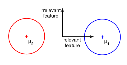
Figure 1: Illustration of the toy experiment for ${{\boldsymbol{\theta}}}=(1,0)^{\top}$.

We generate an $n$-element balanced sample $\mathcal{D}=\{(\boldsymbol{x}_{i},y_{i})\}_{i=1}^{n}$ from two $d=50$-dimensional isotropic Gaussian distributions with equal covariance matrices $C=I_{d\times d}$ and equal, but opposite, means $\mu_{1}=\frac{\rho}{\|{{\boldsymbol{\theta}}}\|_{2}}{{\boldsymbol{\theta}}}$ and $\mu_{2}=-\mu_{1}$. Thereby ${{\boldsymbol{\theta}}}$ is a binary vector, i.e., $\forall i:{\theta_{i}}\in\{0,1\}$, encoding the true underlying data sparsity as follows. Zero components ${\theta_{i}}=0$ clearly imply identical means of the two classes’ distributions in the $i$th feature set; hence the latter does not carry any discriminating information. In summary, the fraction of zero components, $\nu({{\boldsymbol{\theta}}})=1-\frac{1}{d}\sum_{i=1}^{d}{\theta_{i}}$, is a measure for the feature sparsity of the learning problem.

For several values of $\nu$ we generate $m=250$ data sets $\mathcal{D}_{1},\ldots,\mathcal{D}_{m}$ fixing $\rho=1.75$. Then, each feature is input to a linear kernel and the resulting kernel matrices are multiplicatively normalized as described in Section 4.4.2. Hence, $\nu({{\boldsymbol{\theta}}})$ gives the fraction of noise kernels in the working kernel set. Then, classification models are computed by training $\ell_{p}$-norm MKL for $p=1,4/3,2,4,\infty$ on each $\mathcal{D}_{i}$. Soft margin parameters $C$ are tuned on independent $10,000$-elemental validation sets by grid search over $C\in 10^{[-4,3.5,\ldots,0]}$ (optimal $C$s are attained in the interior of the grid). The relative duality gaps were optimized up to a precision of $10^{-3}$. We report on test errors evaluated on $10,000$-elemental independent test sets and pure mean $\ell_{2}$ model errors of the computed kernel mixtures, that is ${\rm ME}({\widehat{{\boldsymbol{\theta}}}})=\|\zeta({\widehat{{\boldsymbol{\theta}}}})-\zeta({{\boldsymbol{\theta}}})\|_{2}$, where $\zeta(\boldsymbol{x})=\frac{\boldsymbol{x}}{\|\boldsymbol{x}\|_{2}}$.

The results are shown in Fig. 2 for $n=50$ and $n=800$, where the figures on the left show the test errors and the ones on the right the model errors ${\rm ME}({\widehat{{\boldsymbol{\theta}}}})$. Regarding the latter, model errors reflect the corresponding test errors for $n=50$. This observation can be explained by statistical learning theory. The minimizer of the empirical risk performs unstable for small sample sizes and the model selection results in a strongly regularized hypothesis, leading to the observed agreement between test error and model error.

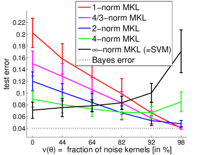
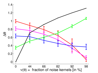
Figure 2: Results of the artificial experiment for sample sizes of $n=50$ (top) and $n=800$ (below) training instances in terms of test errors (left) and mean $\ell_{2}$ model errors ${\rm ME}({\widehat{{\boldsymbol{\theta}}}})$ (right).

Unsurprisingly, $\ell_{1}$ performs best and reaches the Bayes error in the sparse scenario, where only a single kernel carries the whole discriminative information of the learning problem. However, in the other scenarios it mostly performs worse than the other MKL variants. This is remarkable because the underlying ground truth, i.e. the vector ${{\boldsymbol{\theta}}}$, is sparse in all but the uniform scenario. In other words, selecting this data set may imply a bias towards $\ell_{1}$-norm. In contrast, the vanilla SVM using an unweighted sum kernel performs best when all kernels are equally informative, however, its performance does not approach the Bayes error rate. This is because it corresponds to a $\ell_{2,2}$-block norm regularization (see Sect. 4.5) but for a truly uniform regularization a $\ell_{\infty}$-block norm penalty (as employed in Nath et al., 2009) would be needed. This indicates a limitation of our framework; it shall, however, be kept in mind that such a uniform scenario might quite artificial. The non-sparse $\ell_{4}$- and $\ell_{2}$-norm MKL variants perform best in the balanced scenarios, i.e., when the noise level is ranging in the interval 64%-92%. Intuitively, the non-sparse $\ell_{4}$-norm MKL is the most robust MKL variant, achieving a test error of less than $10\%$ in all scenarios. Tuning the sparsity parameter $p$ for each experiment, $\ell_{p}$-norm MKL achieves the lowest test error across all scenarios.

When the sample size is increased to $n=800$ training instances, test errors decrease significantly. Nevertheless, we still observe differences of up to 1% test error between the best ($\ell_{\infty}$-norm MKL) and worst ($\ell_{1}$-norm MKL) prediction model in the two most non-sparse scenarios. Note that all $\ell_{p}$-norm MKL variants perform well in the sparse scenarios. In contrast with the test errors, the mean model errors depicted in Figure 2 (bottom, right) are relatively high. Similarly to above reasoning, this discrepancy can be explained by the minimizer of the empirical risk becoming stable when increasing the sample size (see theoretical Analysis in Appendix A, where we show that speed of the minimizer becoming stable is $O(1/\sqrt{n})$). Again, $\ell_{p}$-norm MKL achieves the smallest test error for all scenarios for appropriately chosen $p$ and for a fixed $p$ across all experiments, the non-sparse $\ell_{4}$-norm MKL performs the most robustly.

In summary, the choice of the norm parameter $p$ is important for small sample sizes, whereas its impact decreases with an increase of the training data. As expected, sparse MKL performs best in sparse scenarios, while non-sparse MKL performs best in moderate or non-sparse scenarios, and for uniform scenarios the unweighted-sum kernel SVM performs best. For appropriately tuning the norm parameter, $\ell_{p}$-norm MKL proves robust in all scenarios.

5.2 Protein Subcellular Localization—a Sparse Scenario

The prediction of the subcellular localization of proteins is one of the rare empirical success stories of $\ell_{1}$-norm-regularized MKL (Ong and Zien, 2008; Zien and Ong, 2007): after defining 69 kernels that capture diverse aspects of protein sequences, $\ell_{1}$-norm-MKL could raise the predictive accuracy significantly above that of the unweighted sum of kernels, and thereby also improve on established prediction systems for this problem. This has been demonstrated on 4 data sets, corresponding to 4 different sets of organisms (plants, non-plant eukaryotes, Gram-positive and Gram-negative bacteria) with differing sets of relevant localizations. In this section, we investigate the performance of non-sparse MKL on the same 4 data sets.

We downloaded the kernel matrices of all 4 data sets. The kernel matrices are multiplicatively normalized as described in Section 4.4.2. The experimental setup used here is related to that of Ong and Zien (2008), although it deviates from it in several details. For each data set, we perform the following steps for each of the 30 predefined splits in training set and test set (downloaded from the same URL): We consider norms $p\in\{1,32/31,16/15,8/7,4/3,2,4,8,\infty\}$ and regularization constants $C\in\{1/32,1/8,1/2,1,2,4,8,32,128\}$. For each parameter setting $(p,C)$, we train $\ell_{p}$-norm MKL using a 1-vs-rest strategy on the training set. The predictions on the test set are then evaluated w.r.t. average (over the classes) MCC (Matthews correlation coefficient). As we are only interested in the influence of the norm on the performance, we forbear proper cross-validation (the so-obtained systematical error affects all norms equally). Instead, for each of the 30 data splits and for each $p$, the value of $C$ that yields the highest MCC is selected. Thus we obtain an optimized $C$ and $MCC$ value for each combination of data set, split, and norm $p$. For each norm, the final $MCC$ value is obtained by averaging over the data sets and splits (i.e., $C$ is selected to be optimal for each data set and split).

The results, shown in Table 1, indicate that indeed, with proper choice of a non-sparse regularizer, the accuracy of $\ell_{1}$-norm can be recovered. On the other hand, non-sparse MKL can approximate the $\ell_{1}$-norm arbitrarily close, and thereby approach the same results. However, even when $1$-norm is clearly superior to $\infty$-norm, as for these 4 data sets, it is possible that intermediate norms perform even better. As the table shows, this is indeed the case for the PSORT data sets, albeit only slightly and not significantly so.

Table 1: Results for Protein Subcellular Localization. For each of the 4 data sets (rows) and each considered norm (columns), we present a measure of prediction error together with its standard error. As measure of prediction error we use 1 minus the average MCC, displayed as percentage.

$\ell_{p}$-norm	$1$	$32/31$	$16/15$	$8/7$	$4/3$	$2$	$4$	$8$	$16$	$\infty$
plant	8.18	8.22	8.20	8.21	8.43	9.47	11.00	11.61	11.91	11.85
std. err.	$\pm$0.47	$\pm$0.45	$\pm$0.43	$\pm$0.42	$\pm$0.42	$\pm$0.43	$\pm$0.47	$\pm$0.49	$\pm$0.55	$\pm$0.60
nonpl	8.97	9.01	9.08	9.19	9.24	9.43	9.77	10.05	10.23	10.33
std. err.	$\pm$0.26	$\pm$0.25	$\pm$0.26	$\pm$0.27	$\pm$0.29	$\pm$0.32	$\pm$0.32	$\pm$0.32	$\pm$0.32	$\pm$0.31
psortNeg	9.99	9.91	9.87	10.01	10.13	11.01	12.20	12.73	13.04	13.33
std. err.	$\pm$0.35	$\pm$0.34	$\pm$0.34	$\pm$0.34	$\pm$0.33	$\pm$0.32	$\pm$0.32	$\pm$0.34	$\pm$0.33	$\pm$0.35
psortPos	13.07	13.01	13.41	13.17	13.25	14.68	15.55	16.43	17.36	17.63
std. err.	$\pm$0.66	$\pm$0.63	$\pm$0.67	$\pm$0.62	$\pm$0.61	$\pm$0.67	$\pm$0.72	$\pm$0.81	$\pm$0.83	$\pm$0.80

We briefly mention that the superior performance of $\ell_{p\approx 1}$-norm MKL in this setup is not surprising. There are four sets of 16 kernels each, in which each kernel picks up very similar information: they only differ in number and placing of gaps in all substrings of length 5 of a given part of the protein sequence. The situation is roughly analogous to considering (inhomogeneous) polynomial kernels of different degrees on the same data vectors. This means that they carry large parts of overlapping information. By construction, also some kernels (those with less gaps) in principle have access to more information (similar to higher degree polynomials including low degree polynomials). Further, Ong and Zien (2008) studied single kernel SVMs for each kernel individually and found that in most cases the 16 kernels from the same subset perform very similarly. This means that each set of 16 kernels is highly redundant and the excluded parts of information are not very discriminative. This renders a non-sparse kernel mixture ineffective. We conclude that $\ell_{1}$-norm must be the best prediction model.

5.3 Gene Start Recognition—a Weighted Non-Sparse Scenario

This experiment aims at detecting transcription start sites (TSS) of RNA Polymerase II binding genes in genomic DNA sequences. Accurate detection of the transcription start site is crucial to identify genes and their promoter regions and can be regarded as a first step in deciphering the key regulatory elements in the promoter region that determine transcription.

Transcription start site finders exploit the fact that the features of promoter regions and the transcription start sites are different from the features of other genomic DNA (Bajic et al., 2004). Many such detectors thereby rely on a combination of feature sets which makes the learning task appealing for MKL. For our experiments we use the data set from Sonnenburg et al. (2006b) which contains a curated set of 8,508 TSS annotated genes utilizing dbTSS version 4 (Suzuki et al., 2002) and refseq genes. These are translated into positive training instances by extracting windows of size $[-1000,+1000]$ around the TSS. Similar to Bajic et al. (2004), 85,042 negative instances are generated from the interior of the gene using the same window size.

Following Sonnenburg et al. (2006b), we employ five different kernels representing the TSS signal (weighted degree with shift), the promoter (spectrum), the 1st exon (spectrum), angles (linear), and energies (linear). Optimal kernel parameters are determined by model selection in Sonnenburg et al. (2006b). The kernel matrices are spherically normalized as described in section 4.4.2. We reserve 13,000 and 20,000 randomly drawn instances for validation and test sets, respectively, and use the remaining 60,000 as the training pool. Soft margin parameters $C$ are tuned on the validation set by grid search over $C\in 2^{[-2,-1,\ldots,5]}$ (optimal $C$s are attained in the interior of the grid). Figure 3 shows test errors for varying training set sizes drawn from the pool; training sets of the same size are disjoint. Error bars indicate standard errors of repetitions for small training set sizes.

Regardless of the sample size, $\ell_{1}$-norm MKL is significantly outperformed by the sum-kernel. On the contrary, non-sparse MKL significantly achieves higher AUC values than the $\ell_{\infty}$-norm MKL for sample sizes up to 20k. The scenario is well suited for $\ell_{2}$-norm MKL which performs best. Finally, for 60k training instances, all methods but $\ell_{1}$-norm MKL yield the same performance. Again, the superior performance of non-sparse MKL is remarkable, and of significance for the application domain: the method using the unweighted sum of kernels (Sonnenburg et al., 2006b) has recently been confirmed to be leading in a comparison of 19 state-of-the-art promoter prediction programs (Abeel et al., 2009), and our experiments suggest that its accuracy can be further elevated by non-sparse MKL.

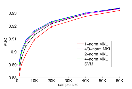
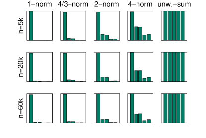
Figure 3: (left) Area under ROC curve (AUC) on test data for TSS recognition as a function of the training set size. Notice the tiny bars indicating standard errors w.r.t. repetitions on disjoint training sets. (right) Corresponding kernel mixtures. For $p=1$ consistent sparse solutions are obtained while the optimal $p=2$ distributes weights on the weighted degree and the 2 spectrum kernels in good agreement to (Sonnenburg et al., 2006b).

We give a brief explanation of the reason for optimality of a non-sparse $\ell_{p}$-norm in the above experiments. It has been shown by Sonnenburg et al. (2006b) that there are three highly and two moderately informative kernels. We briefly recall those results by reporting on the AUC performances obtained from training a single-kernel SVM on each kernel individually: TSS signal $0.89$, promoter $0.86$, 1st exon $0.84$, angles $0.55$, and energies $0.74$, for fixed sample size $n=2000$. While non-sparse MKL distributes the weights over all kernels (see Fig. 3), sparse MKL focuses on the best kernel. However, the superior performance of non-sparse MKL means that dropping the remaining kernels is detrimental, indicating that they may carry additional discriminative information.

To investigate this hypothesis we computed the pairwise alignments of the centered kernel matrices, i.e., $\mathcal{A}(i,j)=\frac{<K_{i},K_{j}>_{F}}{\|K_{i}\|_{F}\|K_{j}\|_{F}}$, with respect to the Frobenius dot product (e.g., Golub and van Loan, 1996). The computed alignments are shown in Fig. 4. One can observe that the three relevant kernels are highly aligned as expected since they are correlated via the labels.

However, the energy kernel shows only a slight correlation with the remaining kernels, which is surprisingly little compared to its single kernel performance (AUC=$0.74$). We conclude that this kernel carries complementary and orthogonal information about the learning problem and should thus be included in the resulting kernel mixture. This is precisely what is done by non-sparse MKL, as can be seen in Fig. 3(right), and the reason for the empirical success of non-sparse MKL on this data set.

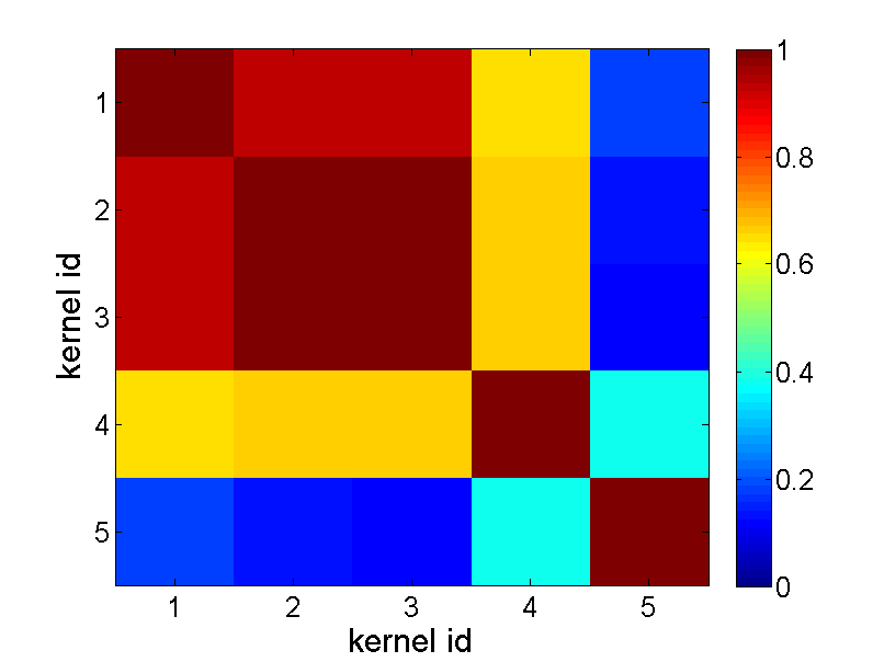
Figure 4: Pairwise alignments of the kernel matrices are shown for the gene start recognition experiment. From left to right, the ordering of the kernel matrices is TSS signal, promoter, 1st exon, angles, and energies. The first three kernels are highly correlated, as expected by their high AUC performances (AUC=$0.84$–$0.89$) and the angle kernel correlates decently (AUC=$0.55$). Surprisingly, the energy kernel correlates only few, despite a descent AUC of $0.74$.

5.4 Reconstruction of Metabolic Gene Network—a Uniformly Non-Sparse Scenario

In this section, we apply non-sparse MKL to a problem originally studied by Yamanishi et al. (2005). Given 668 enzymes of the yeast Saccharomyces cerevisiae and 2782 functional relationships extracted from the KEGG database (Kanehisa et al., 2004), the task is to predict functional relationships for unknown enzymes. We employ the experimental setup of Bleakley et al. (2007) who phrase the task as graph-based edge prediction with local models by learning a model for each of the 668 enzymes. They provided kernel matrices capturing expression data (EXP), cellular localization (LOC), and the phylogenetic profile (PHY); additionally we use the integration of the former 3 kernels (INT) which matches our definition of an unweighted-sum kernel.

Following Bleakley et al. (2007), we employ a $5$-fold cross validation; in each fold we train on average 534 enzyme-based models; however, in contrast to Bleakley et al. (2007) we omit enzymes reacting with only one or two others to guarantee well-defined problem settings. As Table 2 shows, this results in slightly better AUC values for single kernel SVMs where the results by Bleakley et al. (2007) are shown in brackets.

As already observed (Bleakley et al., 2007), the unweighted-sum kernel SVM performs best. Although its solution is well approximated by non-sparse MKL using large values of $p$, $\ell_{p}$-norm MKL is not able to improve on this $p=\infty$ result. Increasing the number of kernels by including recombined and product kernels does improve the results obtained by MKL for small values of $p$, but the maximal AUC values are not statistically significantly different from those of $\ell_{\infty}$-norm MKL. We conjecture that the performance of the unweighted-sum kernel SVM can be explained by all three kernels performing well invidually. Their correlation is only moderate, as shown in Fig. 5, suggesting that they contain complementary information. Hence, downweighting one of those three orthogonal kernels leads to a decrease in performance, as observed in our experiments. This explains why $\ell_{\infty}$-norm MKL is the best prediction model in this experiment.

Table 2: Results for the reconstruction of a metabolic gene network. Results by Bleakley et al. (2007) for single kernel SVMs are shown in brackets.

	AUC $\pm$ stderr
EXP	$71.69\pm 1.1$     ($69.3\pm 1.9$)
LOC	$58.35\pm 0.7$     ($56.0\pm 3.3$)
PHY	$73.35\pm 1.9$     ($67.8\pm 2.1$)
INT ($\infty$-norm MKL)	$\mathbf{82.94}\pm\mathbf{1.1}$     ($\mathbf{82.1}\pm\mathbf{2.2}$)
$1$-norm MKL	$75.08\pm 1.4$
${4/3}$-norm MKL	$78.14\pm 1.6$
$2$-norm MKL	$80.12\pm 1.8$
$4$-norm MKL	$81.58\pm 1.9$
$8$-norm MKL	$81.99\pm 2.0$
$10$-norm MKL	$\mathbf{82.02}\pm\mathbf{2.0}$
Recombined and product kernels
$1$-norm MKL	$79.05\pm 0.5$
$4/3$-norm MKL	$80.92\pm 0.6$
$2$-norm MKL	$81.95\pm 0.6$
$4$-norm MKL	$\mathbf{83.13}\pm\mathbf{0.6}$

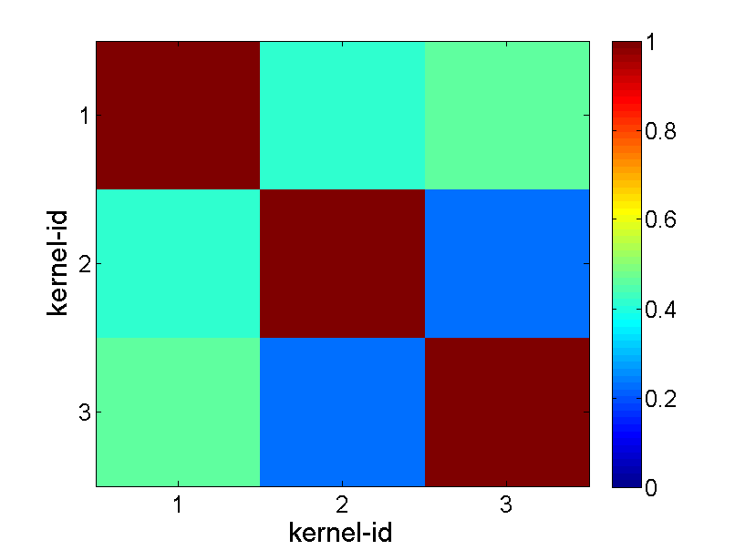
Figure 5: Pairwise alignments of the kernel matrices are shown for the metabolic gene network experiment. From left to right, the ordering of the kernel matrices is EXP, LOC, and PHY. One can see that all kernel matrices are equally correlated. Generally, the alignments are relatively low, suggesting that combining all kernels with equal weights is beneficial.

5.5 Execution Time

In this section we demonstrate the efficiency of our implementations of non-sparse MKL. We experiment on the MNIST data set, where the task is to separate odd vs. even digits. The digits in this $n=60,000$-elemental data set are of size 28x28 leading to $d=784$ dimensional examples. We compare our analytical solver for non-sparse MKL (Section 4.1–4.2) with the state-of-the art for $\ell_{1}$-norm MKL, namely SimpleMKL (Rakotomamonjy et al., 2008), HessianMKL (Chapelle and Rakotomamonjy, 2008), SILP-based wrapper, and SILP-based chunking optimization (Sonnenburg et al., 2006a). We also experiment with the analytical method for $p=1$, although convergence is only guaranteed by our Theorem 4 for $p>1$. We also compare to the semi-infinite program (SIP) approach to $\ell_{p}$-norm MKL presented in Kloft et al. (2009a). In addition, we solve standard SVMs using the unweighted-sum kernel ($\ell_{\infty}$-norm MKL) as baseline.

We experiment with MKL using precomputed kernels (excluding the kernel computation time from the timings) and MKL based on on-the-fly computed kernel matrices measuring training time including kernel computations. Naturally, runtimes of on-the-fly methods should be expected to be higher than the ones of the precomputed counterparts. We optimize all methods up to a precision of $10^{-3}$ for the outer SVM-$\varepsilon$ and $10^{-5}$ for the “inner” SIP precision, and computed relative duality gaps. To provide a fair stopping criterion to SimpleMKL and HessianMKL, we set their stopping criteria to the relative duality gap of their $\ell_{1}$-norm SILP counterpart. SVM trade-off parameters are set to $C=1$ for all methods.

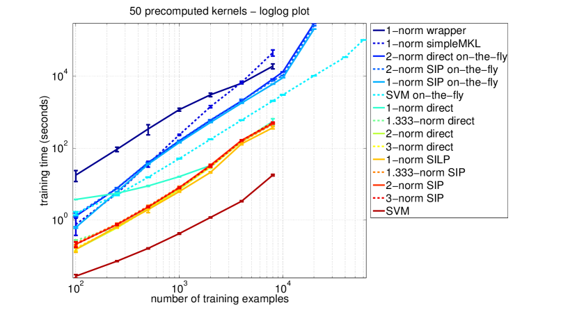
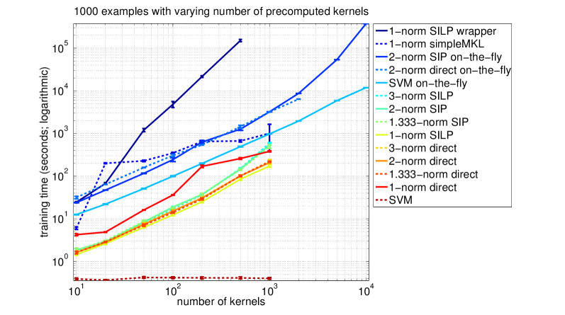
Figure 6: Execution times of SVM and $\ell_{p}$-norm MKL based on interleaved optimization via analytical optimization and semi-infinite programming (SIP), respectively, and wrapper-based optimization via SimpleMKL wrapper and SIP wrapper. Top: Training using fixed number of 50 kernels varying training set size. Bottom: For 1000 examples and varying numbers of kernels. Notice the tiny error bars and that these are log-log plots.

Scalability of the Algorithms w.r.t. Sample Size

Figure 6 (top) displays the results for varying sample sizes and 50 precomputed or on-the-fly computed Gaussian kernels with bandwidths $2\sigma^{2}\in 1.2^{0,\dots,49}$. Error bars indicate standard error over 5 repetitions. As expected, the SVM with the unweighted-sum kernel using precomputed kernel matrices is the fastest method. The classical MKL wrapper based methods, SimpleMKL and the SILP wrapper, are the slowest; they are even slower than methods that compute kernels on-the-fly. Note that the on-the-fly methods naturally have higher runtimes because they do not profit from precomputed kernel matrices.

Notably, when considering 50 kernel matrices of size 8,000 times 8,000 (memory requirements about 24GB for double precision numbers), SimpleMKL is the slowest method: it is more than 120 times slower than the $\ell_{1}$-norm SILP solver from Sonnenburg et al. (2006a). This is because SimpleMKL suffers from having to train an SVM to full precision for each gradient evaluation. In contrast, kernel caching and interleaved optimization still allow to train our algorithm on kernel matrices of size $20000\times 20000$, which would usually not completely fit into memory since they require about 149GB.

Non-sparse MKL scales similarly as $\ell_{1}$-norm SILP for both optimization strategies, the analytic optimization and the sequence of SIPs. Naturally, the generalized SIPs are slightly slower than the SILP variant, since they solve an additional series of Taylor expansions within each ${\boldsymbol{\theta}}$-step. HessianMKL ranks in between on-the-fly and non-sparse interleaved methods.

Scalability of the Algorithms w.r.t. the Number of Kernels

Figure 6 (bottom) shows the results for varying the number of precomputed and on-the-fly computed RBF kernels for a fixed sample size of 1000. The bandwidths of the kernels are scaled such that for $M$ kernels $2\sigma^{2}\in 1.2^{0,\dots,M-1}$. As expected, the SVM with the unweighted-sum kernel is hardly affected by this setup, taking an essentially constant training time. The $\ell_{1}$-norm MKL by Sonnenburg et al. (2006a) handles the increasing number of kernels best and is the fastest MKL method. Non-sparse approaches to MKL show reasonable run-times, being just slightly slower. Thereby the analytical methods are somewhat faster than the SIP approaches. The sparse analytical method performs worse than its non-sparse counterpart; this might be related to the fact that convergence of the analytical method is only guaranteed for $p>1$. The wrapper methods again perform worst.

However, in contrast to the previous experiment, SimpleMKL becomes more efficient with increasing number of kernels. We conjecture that this is in part owed to the sparsity of the best solution, which accommodates the $l_{1}$-norm model of SimpleMKL. But the capacity of SimpleMKL remains limited due to memory restrictions of the hardware. For example, for storing 1,000 kernel matrices for 1,000 data points, about 7.4GB of memory are required. On the other hand, our interleaved optimizers which allow for effective caching can easily cope with 10,000 kernels of the same size (74GB). HessianMKL is considerably faster than SimpleMKL but slower than the non-sparse interleaved methods and the SILP. Similar to SimpleMKL, it becomes more efficient with increasing number of kernels but eventually runs out of memory.

Overall, our proposed interleaved analytic and cutting plane based optimization strategies achieve a speedup of up to one and two orders of magnitude over HessianMKL and SimpleMKL, respectively. Using efficient kernel caching, they allow for truely large-scale multiple kernel learning well beyond the limits imposed by having to precompute and store the complete kernel matrices. Finally, we note that performing MKL with 1,000 precomputed kernel matrices of size 1,000 times 1,000 requires less than 3 minutes for the SILP. This suggests that it focussing future research efforts on improving the accuracy of MKL models may pay off more than further accelerating the optimization algorithm.

6 Conclusion

We translated multiple kernel learning into a regularized risk minimization problem for arbitrary convex loss functions, Hilbertian regularizers, and arbitrary-norm penalties on the mixing coefficients. Our formulation can be motivated by both Tikhonov and Ivanov regularization approaches, the latter one having an additional regularization parameter. Applied to previous MKL research, our framework provides a unifying view and shows that so far seemingly different MKL approaches are in fact equivalent.

Furthermore, we presented a general dual formulation of multiple kernel learning that subsumes many existing algorithms. We devised an efficient optimization scheme for non-sparse $\ell_{p}$-norm MKL with $p\geq 1$, based on an analytic update for the mixing coefficients, and interleaved with chunking-based SVM training to allow for application at large scales. It is an open question whether our algorithmic approach extends to more general norms. Our implementations are freely available and included in the SHOGUN toolbox. The execution times of our algorithms revealed that the interleaved optimization vastly outperforms commonly used wrapper approaches. Our results and the scalability of our MKL approach pave the way for other real-world applications of multiple kernel learning.

In order to empirically validate our $\ell_{p}$-norm MKL model, we applied it to artificially generated data and real-world problems from computational biology. For the controlled toy experiment, where we simulated various levels of sparsity, $\ell_{p}$-norm MKL achieved a low test error in all scenarios for scenario-wise tuned parameter $p$. Moreover, we studied three real-world problems showing that the choice of the norm is crucial for state-of-the art performance. For the TSS recognition, non-sparse MKL raised the bar in predictive performance, while for the other two tasks either sparse MKL or the unweighted-sum mixture performed best. In those cases the best solution can be arbitrarily closely approximated by $\ell_{p}$-norm MKL with $1<p<\infty$. Hence it seems natural that we observed non-sparse MKL to be never worse than an unweighted-sum kernel or a sparse MKL approach. Moreover, empirical evidence from our experiments along with others suggests that the popular $\ell_{1}$-norm MKL is more prone to bad solutions than higher norms, despite appealing guarantees like the model selection consistency (Bach, 2008).

A first step towards a learning-theoretical understanding of this empirical behaviour may be the convergence analysis undertaken in the appendix of this paper. It is shown that in a sparse scenario $\ell_{1}$-norm MKL converges faster than non-sparse MKL due to a bias that well is well-taylored to the ground truth. In their current form the bounds seem to suggest that furthermore, in all other cases, $\ell_{1}$-norm MKL is at least as good as non-sparse MKL. However this would be inconsistent with both the no-free-lunch theorem and our empirical results, which indicate that there exist scenarios in which non-sparse models are advantageous. We conjecture that the non-sparse bounds are not yet tight and need further improvement, for which the results in Appendix A may serve as a starting point.

A related—and obtruding!—question is whether the optimality of the parameter $p$ can retrospectively be explained or, more profitably, even be estimated in advance. Clearly, cross-validation based model selection over the choice of $p$ will inevitably tell us which cases call for sparse or non-sparse models. The analyses of our real-world applications suggests that both the correlation amongst the kernels with each other and their correlation with the target (i.e., the amount of discriminative information that they carry) play a role in the distinction of sparse from non-sparse scenarios. However, the exploration of theoretical explanations is beyond the scope of this work. Nevertheless, we remark that even completely redundant but uncorrelated kernels may improve the predictive performance of a model, as averaging over several of them can reduce the variance of the predictions (cf., e.g., Guyon and Elisseeff, 2003, Sect. 3.1). Intuitively speaking, we observe clearly that in some cases all features, even though they may contain redundant information, should be kept, since putting their contributions to zero worsens prediction, i.e. all of them are informative to our MKL models.

Finally, we would like to note that it may be worthwhile to rethink the current strong preference for sparse models in the scientific community. Already weak connectivity in a causal graphical model may be sufficient for all variables to be required for optimal predictions (i.e., to have non-zero coefficients), and even the prevalence of sparsity in causal flows is being questioned (e.g., for the social sciences Gelman (2010) argues that ”There are (almost) no true zeros”). A main reason for favoring sparsity may be the presumed interpretability of sparse models. This is not the topic and goal of this article; however we remark that in general the identified model is sensitive to kernel normalization, and in particular in the presence of strongly correlated kernels the results may be somewhat arbitrary, putting their interpretation in doubt. However, in the context of this work the predictive accuracy is of focal interest, and in this respect we demonstrate that non-sparse models may improve quite impressively over sparse ones.

Acknowledgments

The authors wish to thank Vojtech Franc, Peter Gehler, Pavel Laskov, Motoaki Kawanabe, and Gunnar Rätsch for stimulating discussions, and Chris Hinrichs and Klaus-Robert Müller for helpful comments on the manuscript. We acknowledge Peter L. Bartlett and Ulrich Rückert for contributions to parts of an earlier version of the theoretical analysis that appeared at ECML 2010. We thank the anonymous reviewers for comments and suggestions that helped to improve the manuscript. This work was supported in part by the German Bundesministerium für Bildung und Forschung (BMBF) under the project REMIND (FKZ 01-IS07007A), and by the FP7-ICT program of the European Community, under the PASCAL2 Network of Excellence, ICT-216886. Sören Sonnenburg acknowledges financial support by the German Research Foundation (DFG) under the grant MU 987/6-1 and RA 1894/1-1, and Marius Kloft acknowledges a scholarship by the German Academic Exchange Service (DAAD).

A Theoretical Analysis

In this section we present a theoretical analysis of $\ell_{p}$-norm MKL, based on Rademacher complexities. We prove a theorem that converts any Rademacher-based generalization bound on $\ell_{1}$-norm MKL into a generalization bound for $\ell_{p}$-norm MKL (and even more generally: arbitrary-norm MKL). Remarkably this $\ell_{1}$-to-$\ell_{p}$ conversion is obtained almost without any effort: by a simple 5-line proof. The proof idea is based on Kloft et al. (2010). We remark that an $\ell_{p}$-norm MKL bound was already given in Cortes et al. (2010a), but first their bound is only valid for the special cases $p=n/(n-1)$ for $n=1,2,\ldots$, and second it is not tight for all $p$, as it diverges to infinity when $p>1$ and $p$ approaches one. By contrast, beside a rather unsubstantial $\log(M)$-factor, our result matches the best known lower bounds, when $p$ approaches one.

Let us start by defining the hypothesis set that we want to investigate. Following Cortes et al. (2010a), we consider the following hypothesis class for $p\in[1,\infty]$:

$$H_{M}^{p}:=\left\{h:\mathcal{X}\rightarrow\mathbb{R}~{}\bigg{|}~{}h(\boldsymbol{x})=\sum_{m=1}^{M}\sqrt{\theta_{m}}\langle\boldsymbol{w}_{m},\psi_{m}(\boldsymbol{x})\rangle_{\mathcal{H}_{m}},~{}\|\boldsymbol{w}\|_{\mathcal{H}}\leq 1,~{}\|{\boldsymbol{\theta}}\|_{p}\leq 1\right\}.$$

Solving our primal MKL problem (P) corresponds to empirical risk minimization in the above hypothesis class. We are thus interested in bounding the generalization error of the above class w.r.t. an i.i.d. sample $(\boldsymbol{x}_{1},y_{1}),...,(\boldsymbol{x}_{n},y_{n})\in\mathcal{X}\times\{-1,1\}$ from an arbitrary distribution $P=P_{X}\times P_{Y}$. In order to do so, we compute the Rademacher complexity,

$${\mathscr{R}}(H_{M}^{p}):=\mathbb{E}\bigg{[}\sup_{h\in H_{M}^{p}}\frac{1}{n}\sum_{i=1}^{n}\sigma_{i}h(\boldsymbol{x}_{i})\bigg{]},$$

where $\sigma_{1},\ldots,\sigma_{n}$ are independent Rademacher variables (i.e. they obtain the values -1 or +1 with the same probability 0.5) and the $\mathbb{E}$ is the expectation operator that removes the dependency on all random variables, i.e. $\sigma_{i}$, $\boldsymbol{x}_{i}$, and $y_{i}$ ($i=1,...,n$). If the Rademacher complexity is known, there is a large body of results which can be used to bound the generalization error (e.g., Koltchinskii and Panchenko, 2002; Bartlett and Mendelson, 2002).

We now show a simple $\ell_{1}$-to-$\ell_{p}$ conversion technique for the Rademacher complexity, which is the main result of this section:

Theorem 6 ($\ell_{1}$-to-$\ell_{p}$ Conversion).

For any sample of size $n$ and $p\in[1,\infty]$, the Rademacher complexity of the hypothesis set $H_{M}^{p}$ can be bounded as follows:

$${\mathscr{R}}(H_{M}^{p})\leq\sqrt{M^{1/p^{*}}}{\mathscr{R}}(H_{M}^{1}),$$

where $p^{*}:=p/(p-1)$ is the conjugated exponent of $p$.

Proof.

By Hölder’s inequality (e.g., Steele, 2004), we have

$$\forall{\boldsymbol{\theta}}\in\mathbb{R}^{M}:~{}\quad\|{\boldsymbol{\theta}}\|_{1}=\mathbf{1}^{\top}{\boldsymbol{\theta}}\leq\|\mathbf{1}\|_{p^{*}}\|{\boldsymbol{\theta}}\|_{p}=M^{1/p^{*}}\|{\boldsymbol{\theta}}\|_{p}~{}.\hskip 14.22636pt$$ (32)

Hence,

$${\mathscr{R}}(H_{M}^{p}) \stackrel{{\scriptstyle\rm Def.}}{{=}} \mathbb{E}\bigg{[}\sup_{\boldsymbol{w}:\|\boldsymbol{w}\|_{\mathcal{H}}\leq 1,~{}{\boldsymbol{\theta}}:\|{\boldsymbol{\theta}}\|_{p}\leq 1}\frac{1}{n}\sum_{i=1}^{n}\sigma_{i}\sum_{m=1}^{M}\sqrt{\theta_{m}}\langle\boldsymbol{w}_{m},\psi_{m}(\boldsymbol{x}_{i})\rangle_{\mathcal{H}_{m}}\bigg{]}$$

$$\stackrel{{\scriptstyle\eqref{hoelder_trick}}}{{\leq}} \mathbb{E}\bigg{[}\sup_{\boldsymbol{w}:\|\boldsymbol{w}\|_{\mathcal{H}}\leq 1,~{}{\boldsymbol{\theta}}:\|{\boldsymbol{\theta}}\|_{1}\leq M^{1/p^{*}}}\frac{1}{n}\sum_{i=1}^{n}\sigma_{i}\sum_{m=1}^{M}\sqrt{\theta_{m}}\langle\boldsymbol{w}_{m},\psi_{m}(\boldsymbol{x}_{i})\rangle_{\mathcal{H}_{m}}\bigg{]}$$

$$= \mathbb{E}\bigg{[}\sup_{\boldsymbol{w}:\|\boldsymbol{w}\|_{\mathcal{H}}\leq 1,~{}{\boldsymbol{\theta}}:\|{\boldsymbol{\theta}}\|_{1}\leq 1}\frac{1}{n}\sum_{i=1}^{n}\sigma_{i}\sum_{m=1}^{M}\sqrt{\theta_{m}M^{1/p^{*}}}\langle\boldsymbol{w}_{m},\psi_{m}(\boldsymbol{x})\rangle_{\mathcal{H}_{m}}\bigg{]}$$

$$\stackrel{{\scriptstyle\rm Def.}}{{=}} \sqrt{M^{1/p^{*}}}{\mathscr{R}}(H_{M}^{1}).$$

∎

Remark 7.

More generally we have that for any norm $\|\cdot\|_{\star}$ on $\mathbb{R}^{M}$, because all norms on $\mathbb{R}^{M}$ are equivalent (e.g., Rudin, 1991), there exists a $c_{\star}\in\mathbb{R}$ such that

$${\mathscr{R}}(H_{M}^{p})\leq c_{\star}{\mathscr{R}}(H_{M}^{\star}).$$

This means the conversion technique extends to arbitrary norms: for any given norm ${\|\cdot\|_{\star}}$, we can convert any bound on ${\mathscr{R}}(H_{M}^{p})$ into a bound on the Rademacher complexity ${\mathscr{R}}(H_{M}^{\star})$ of hypothesis set induced by $\|\cdot\|_{\star}$.

A nice thing about the above bound is that we can make use of any existing bound on the Rademacher complexity of $H_{M}^{1}$ in order to obtain a generalization bound for $H_{M}^{p}$. This fact is illustrated in the following. For example, the tightest result bounding ${\mathscr{R}}(H_{M}^{1})$ known so far is:

Theorem 8 (Cortes et al. (2010a)).

Let $M>1$ and assume that $k_{m}(\boldsymbol{x},\boldsymbol{x})\leq R^{2}$ for all $\boldsymbol{x}\in\mathcal{X}$ and $m=1,\ldots,M$. Then, for any sample of size $n$, the Rademacher complexity of the hypothesis set $H_{M}^{1}$ can be bounded as follows (where $c:=23/22$):

$${\mathscr{R}}(H_{M}^{1})\leq\sqrt{\frac{ce\lceil\log M\rceil R^{2}}{n}}.$$

The above result directly leads to a $O(\sqrt{\log M})$ bound on the generalization error and thus substantially improves on a series of loose results given within the past years (see Cortes et al., 2010a, and references therein). We can use the above result (or any other similar result) to obtain a bound for $H_{M}^{p}$:

Corollary (of the previous two theorems).

Let $M>1$ and assume that $k_{m}(\boldsymbol{x},\boldsymbol{x})\leq R^{2}$ for all $\boldsymbol{x}\in\mathcal{X}$ and $m=1,\ldots,M$. Then, for any sample of size $n$, the Rademacher complexity of the hypothesis set $H_{M}^{1}$ can be bounded as follows:

$$\forall p\in[1,...,\infty]:\quad{\mathscr{R}}(H_{M}^{p})\leq\sqrt{\frac{ceM^{1/p^{*}}\lceil\log M\rceil R^{2}}{n}},$$

where $p^{*}:=p/(p-1)$ is the conjugated exponent of $p$ and $c:=23/22$.

It is instructive to compare the above bound, which we obtained by our $\ell_{1}$-to-$\ell_{p}$ conversion technique, with the one given in Cortes et al. (2010a): that is ${\mathscr{R}}(H_{M}^{p})\leq\sqrt{\frac{cep^{*}M^{1/p^{*}}R^{2}}{n}}$ for any $p\in[1,...,\infty]$ such that $p^{*}$ is an integer. First, we observe that for $p=2$ the bounds’ rates almost coincide: they only differ by a $\log M$-factor, which is unsubstantial due to the presence of a polynomial term that domiates the asymptotics. Second, we observe that for small $p$ (close to one), the $p^{*}$-factor in the Cortes-bound leads to considerably high constants. When $p$ approaches one, it even diverges to infinity. In contrast, our bound converges to ${\mathscr{R}}(H_{M}^{p})\leq\sqrt{\frac{ce\lceil\log M\rceil R^{2}}{n}}$ when $p$ approaches one, which is precisely the tight 1-norm bound of Thm. 8. Finally, it is also interesting to consider the case $p\geq 2$ (which is not covered by the Cortes et al. (2010a) bound): if we let $p\rightarrow\infty$, we obtain ${\mathscr{R}}(H_{M}^{p})\leq\sqrt{\frac{ceM\lceil\log M\rceil R^{2}}{n}}$. Beside the unsubstantial $\log M$-factor, our so obtained ${\cal O}\left(\sqrt{M}\ln(M)\right)$ bound matches the well-known ${\cal O}\left(\sqrt{M}\right)$ lower bounds based on the VC-dimension (e.g., Devroye et al., 1996, Section 14).

We now make use of the above analysis of the Rademacher complexity to bound the generalization error. There are many results in the literature that can be employed to this aim. Ours is based on Thm. 7 in Bartlett and Mendelson (2002):

Corollary 9.

Let $M>1$ and $p\in[1,...,\infty]$. Assume that $k_{m}(\boldsymbol{x},\boldsymbol{x})\leq R^{2}$ for all $\boldsymbol{x}\in\mathcal{X}$ and $m=1,\ldots,M$. Assume the loss $V:\mathbb{R}\rightarrow[0,1]$ is Lipschitz with constant $L$ and $V(t)\geq 1$ for all $t\leq 0$. Set $p^{*}:=p/(p-1)$ and $c:=23/22$. Then, the following holds with probability larger than $1-\delta$ over samples of size $n$ for all classifiers $h\in H_{M}^{p}$:

$$R(h)\leq\widehat{R}(h)+2L\sqrt{\frac{ceM^{1/p^{*}}\lceil\log M\rceil R^{2}}{n}}+\sqrt{\frac{\ln(2/\delta)}{2n}},$$ (33)

where $R(h)={\rm P}\big{[}yh(\boldsymbol{x})\leq 0\big{]}$ is the expected risk w.r.t. 0-1 loss and $\widehat{R}(h)=\frac{1}{n}\sum_{i=1}^{n}V(y_{i}h(x_{i}))$ is the empirical risk w.r.t. loss $V$.

The above theorem is formulated for general Lipschitz loss functions. Since the margin loss $V(t)=\min\big{(}1,[1-t/{\gamma}]_{+}\big{)}$ is Lipschitz with constant $1/\gamma$ and upper bounding the 0-1 loss, it fulfills the preliminaries of the above corollary. Hence, we immediately obtain the following radius-margin bound (see also Koltchinskii and Panchenko, 2002):

Corollary 10 ($\ell_{p}$-norm MKL Radius-Margin Bound).

Fix the margin ${\gamma}>0$. Let $M>1$ and $p\in[1,...,\infty]$. Assume that $k_{m}(\boldsymbol{x},\boldsymbol{x})\leq R^{2}$ for all $\boldsymbol{x}\in\mathcal{X}$ and $m=1,\ldots,M$. Set $p^{*}:=p/(p-1)$ and $c:=23/22$. Then, the following holds with probability larger than $1-\delta$ over samples of size $n$ for all classifiers $h\in H_{M}^{p}$:

$$R(h)\leq\widehat{R}(h)+\frac{2R}{{\gamma}}\sqrt{\frac{ceM^{1/p^{*}}\lceil\log M\rceil}{n}}+\sqrt{\frac{\ln(2/\delta)}{2n}},$$ (34)

where $R(h)={\rm P}\big{[}yh(\boldsymbol{x})\leq 0\big{]}$ is the expected risk w.r.t. 0-1 loss and $\widehat{R}(h)=\frac{1}{n}\sum_{i=1}^{n}\min\big{(}1,[1-y_{i}h(\boldsymbol{x}_{i})/{\gamma}]_{+}\big{)}$ the empirical risk w.r.t. margin loss.

Finally, we would like to point out that, for reasons stated in Remark 7, our $\ell_{1}$-to-$\ell_{p}$ conversion technique lets us easily extend the above bounds to norms different than $\ell_{p}$ . This includes, for example, block norms and sums of block norms as used in elastic-net regularization (see Kloft et al., 2010, for such bounds), but also non-isotropic norms such as weighted $\ell_{p}$-norms.

A.1 Case-based Analysis of a Sparse and a Non-Sparse Scenario

From the results given in the last section it seems that it is beneficial to use a sparsity-inducing $\ell_{1}$-norm penalty when learning with multiple kernels. This however somewhat contradicts our empirical evaluation, which indicated that the optimal norm parameter $p$ depends on the true underlying sparsity of the problem. Indeed, as we show below, a refined theoretical analysis supports this intuitive claim. We show that if the underlying truth is uniformly non-sparse, then a priori there is no $p$-norm which is more promising than another one. On the other hand, we illustrate that in a sparse scenario, the sparsity-inducing $\ell_{1}$-norm indeed can be beneficial.

We start by reparametrizing our hypothesis set based on block norms: by Prop. 5 it holds that

$$H_{M}^{p}=\left\{h:\mathcal{X}\rightarrow\mathbb{R}~{}\bigg{|}~{}h(\boldsymbol{x})=\sum_{m=1}^{M}\langle\boldsymbol{w}_{m},\psi_{m}(\boldsymbol{x})\rangle_{\mathcal{H}_{m}},~{}\|\boldsymbol{w}\|_{2,q}\leq 1,~{}q:=2p/(p+1)\right\},$$

where $||\boldsymbol{w}||_{2,q}:=\left(\sum_{m=1}^{M}||\boldsymbol{w}_{m}||_{\mathcal{H}_{m}}^{q}\right)^{1/q}$ is the $\ell_{2,q}$-block norm. This means we can equivalently parametrize our hypothesis set in terms of block norms. Second, let us generalize the set by introducing an additional parameter $C$ as follows

$${\text{\small{${}^{C}$}}}{H_{M}^{p}}:=\left\{h:\mathcal{X}\rightarrow\mathbb{R}~{}\bigg{|}~{}h(\boldsymbol{x})=\sum_{m=1}^{M}\langle\boldsymbol{w}_{m},\psi_{m}(\boldsymbol{x})\rangle_{\mathcal{H}_{m}},~{}\|\boldsymbol{w}\|_{2,q}\leq C,~{}q:=2p/(p+1)\right\}.$$

Clearly, ${\text{\small{${}^{C}$}}}H_{M}^{p}=H_{M}^{p}$ for $C=1$, which explains why the parametrization via $C$ is more general. It is straight forward to verify that ${\mathscr{R}}\left({\text{\small{${}^{C}$}}}H_{M}^{p}\right)=C{\mathscr{R}}\left(H_{M}^{p}\right)$ for any $C$. Hence, under the preliminaries of Corollary 9, we have

$$R(h)\leq\widehat{R}(h)+2L\sqrt{\frac{ceM^{1/p^{*}}\lceil\log M\rceil R^{2}C^{2}}{n}}+\sqrt{\frac{\ln(2/\delta)}{2n}}.$$ (35)

We will exploit the above bound in the following two illustrate examples.

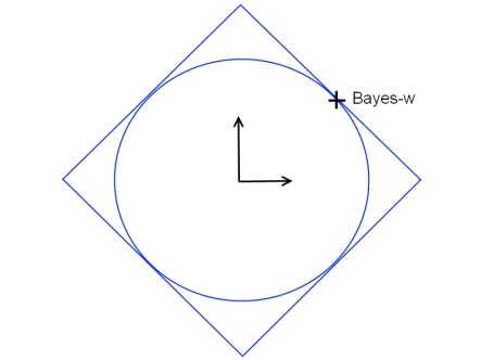
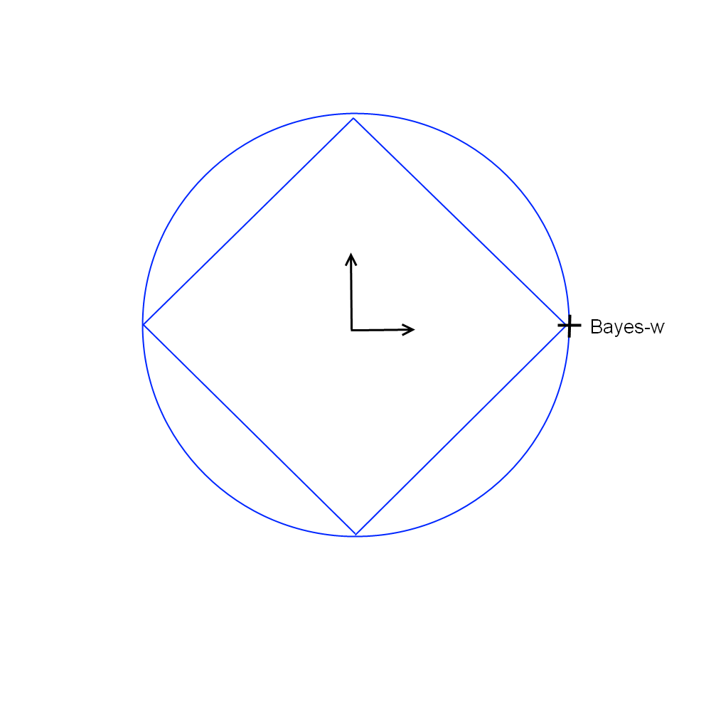
Figure 7: Illustration of the two analyzed cases: a uniformly non-sparse (Example 1, left) and a sparse (Example 2, right) Scenario.

Example 1.

Let the input space be $\mathcal{X}=\mathbb{R}^{M}$, and the feature map be $\psi_{m}(\boldsymbol{x})=x_{m}$ for all $m=1,\ldots,M$ and $\boldsymbol{x}=(x_{1},...,x_{M})\in\mathcal{X}$ (in other words, $\psi_{m}$ is a projection on the $m$th feature). Assume that the Bayes-optimal classifier is given by

$$\boldsymbol{w}_{\rm Bayes}=(1,\ldots,1)^{\top}\in\mathbb{R}^{M}.$$

This means the best classifier possible is uniformly non-sparse (see Fig. 7, left). Clearly, it can be advantageous to work with a hypothesis set that is rich enough to contain the Bayes classifier, i.e. $(1,\ldots,1)^{\top}\in{\text{\small{${}^{C}$}}}H_{M}^{p}$. In our example, this is the case if and only if $\|(1,\ldots,1)^{\top}\|_{2p/(p+1)}\leq C$, which itself is equivalent to $M^{(p+1)/2p}\leq C$. The bound (35) attains its minimal value under the latter constraint for $M^{(p+1)/2p}=C$. Resubstitution into the bound yields

$$R(h)\leq\widehat{R}(h)+2L\sqrt{\frac{ceM^{2}\lceil\log M\rceil R^{2}}{n}}+\sqrt{\frac{\ln(2/\delta)}{2n}}.$$

Interestingly, the obtained bound does not depend on the norm parameter $p$ at all! This means that in this particular (non-sparse) example all $p$-norm MKL variants yield the same generalization bound. There is thus no theoretical evidence which norm to prefer a priori.

Example 2.

In this second example we consider the same input space and kernels as before. But this time we assume a sparse Bayes-optimal classifier (see Fig. 7, right)

$$\boldsymbol{w}_{\rm Bayes}=(1,0,\ldots,0)^{\top}\in\mathbb{R}^{M}.$$

As in the previous example, in order $\boldsymbol{w}_{\rm Bayes}$ to be in the hypothesis set, we have to require $\|(1,0,\ldots,0)^{\top}\|_{2p/(p+1)}\leq C$. But this time this simply solves to $C\geq 1$, which is independent of the norm parameter $p$. Thus, inserting $C=1$ in the bound (35), we obtain

$$R(h)\leq\widehat{R}(h)+2L\sqrt{\frac{ceM^{1/p^{*}}\lceil\log M\rceil R^{2}}{n}}+\sqrt{\frac{\ln(2/\delta)}{2n}},$$

which is precisely the bound of Corollary 9. It is minimized for $p=1$; thus, in this particular sparse example, the bound is considerably smaller for sparse MKL—especially, if the number of kernels is high compared to the sample size. This is also intuitive: if the underlying truth is sparse, we expect a sparsity-inducing norm to match well the ground truth.

We conclude from the previous two examples that the optimal norm parameter $p$ depends on the underlying ground truth: if it is sparse, then choosing a sparse regularization is beneficial; otherwise, any norm $p$ can perform well. I.e., without any domain knowledge there is no norm that a priori should be preferred. Remarkably, this still holds when we increase the number of kernels. This is somewhat contrary to anecdotal reports, which claim that sparsity-inducing norms are beneficial in high (kernel) dimensions. This is because those analyses implicitly assume the ground truth to be sparse. The present paper, however, clearly shows that we might encounter a non-sparse ground truth in practical applications (see experimental section).

B Switching between Tikhonov and Ivanov Regularization

In this appendix, we show a useful result that justifies switching from Tikhonov to Ivanov regularization and vice versa, if the bound on the regularizing constraint is tight. It is the key ingredient of the proof of Theorem 1. We state the result for arbitrary convex functions, so that it can be applied beyond the multiple kernel learning framework of this paper.

Proposition 11.

Let $D\subset\mathbb{R}^{d}$ be a convex set, let $f,g:D\rightarrow\mathbb{R}$ be convex functions. Consider the convex optimization tasks

$$~{}\min_{\boldsymbol{x}\in D}\quad f(\boldsymbol{x})+\sigma g(\boldsymbol{x}),$$ (36a)

$$\min_{\boldsymbol{x}\in D:g(\boldsymbol{x})\leq\tau}\quad\quad\quad f(\boldsymbol{x}).$$ (36b)

Assume that the minima exist and that a constraint qualification holds in (36b), which gives rise to strong duality, e.g., that Slater’s condition is satisfied. Furthermore assume that the constraint is active at the optimal point, i.e.

$$\inf_{\boldsymbol{x}\in D}~{}f(\boldsymbol{x})~{}<~{}\inf_{\boldsymbol{x}\in D:g(\boldsymbol{x})\leq\tau}~{}f(\boldsymbol{x}).$$ (37)

Then we have that for each $\sigma>0$ there exists $\tau>0$—and vice versa—such that OP (36a) is equivalent to OP (36b), i.e., each optimal solution of one is an optimal solution of the other, and vice versa.

Proof.

(a). Let be $\sigma>0$ and $\boldsymbol{x}^{*}$ be the optimal of (36a). We have to show that there exists a $\tau>0$ such that $\boldsymbol{x}^{*}$ is optimal in (36b). We set $\tau=g(\boldsymbol{x}^{*})$. Suppose $\boldsymbol{x}^{*}$ is not optimal in (36b), i.e., it exists $\tilde{\boldsymbol{x}}\in D:g(\tilde{\boldsymbol{x}})\leq\tau$ such that $f(\tilde{\boldsymbol{x}})<f(\boldsymbol{x}^{*})$. Then we have

$$f(\tilde{\boldsymbol{x}})+\sigma g(\tilde{\boldsymbol{x}})<f(\boldsymbol{x}^{*})+\sigma\tau,$$

which by $\tau=g(\boldsymbol{x}^{*})$ translates to

$$f(\tilde{\boldsymbol{x}})+\sigma g(\tilde{\boldsymbol{x}})<f(\boldsymbol{x}^{*})+\sigma g(\boldsymbol{x}^{*}).$$

This contradics the optimality of $\boldsymbol{x}^{*}$ in (36a), and hence shows that $\boldsymbol{x}^{*}$ is optimal in (36b), which was to be shown.
(b). Vice versa, let $\tau>0$ be $\boldsymbol{x}^{*}$ optimal in (36b). The Lagrangian of (36b) is given by

$$\mathcal{L}(\sigma)=f(\boldsymbol{x})+\sigma\left(g(\boldsymbol{x})-\tau\right),\quad\sigma\geq 0.$$

By strong duality $\boldsymbol{x}^{*}$ is optimal in the saddle point problem

$$\sigma^{*}:=\operatorname*{argmax}_{\sigma\geq 0}~{}\min_{\boldsymbol{x}\in D}\quad f(\boldsymbol{x})+\sigma\left(g(\boldsymbol{x})-\tau\right),$$

and by the strong max-min property (cf. (Boyd and Vandenberghe, 2004), p. 238) we may exchange the order of maximization and minimization. Hence $\boldsymbol{x}^{*}$ is optimal in

$$\min_{\boldsymbol{x}\in D}\quad f(\boldsymbol{x})+\sigma^{*}\left(g(\boldsymbol{x})-\tau\right).$$ (38)

Removing the constant term $-\sigma^{*}\tau$, and setting $\sigma=\sigma^{*}$, we have that $\boldsymbol{x}^{*}$ is optimal in (36a), which was to be shown. Moreover by (37) we have that

$$\boldsymbol{x}^{*}\neq\operatorname*{argmin}_{\boldsymbol{x}\in D}f(\boldsymbol{x}),$$

and hence we see from Eq. (38) that $\sigma^{*}>0$, which completes the proof of the proposition. ∎

References

- Abeel et al. (2009) T. Abeel, Y. V. de Peer, and Y. Saeys. Towards a gold standard for promoter prediction evaluation. Bioinformatics, 2009.
- Aflalo et al. (2009) J. Aflalo, A. Ben-Tal, C. Bhattacharyya, J. S. Nath, and S. Raman. Variable sparsity kernel learning—algorithms and applications. Journal of Machine Learning Research, 2009. Submitted 12/2009. Preprint: http://mllab.csa.iisc.ernet.in/vskl.html.
- Argyriou et al. (2008) A. Argyriou, T. Evgeniou, and M. Pontil. Convex multi-task feature learning. Machine Learning, 73(3):243–272, 2008.
- Bach (2009) F. Bach. Exploring large feature spaces with hierarchical multiple kernel learning. In D. Koller, D. Schuurmans, Y. Bengio, and L. Bottou, editors, Advances in Neural Information Processing Systems 21, pages 105–112, 2009.
- Bach (2008) F. R. Bach. Consistency of the group lasso and multiple kernel learning. J. Mach. Learn. Res., 9:1179–1225, 2008.
- Bach et al. (2004) F. R. Bach, G. R. G. Lanckriet, and M. I. Jordan. Multiple kernel learning, conic duality, and the SMO algorithm. In Proc. 21st ICML. ACM, 2004.
- Bajic et al. (2004) V. B. Bajic, S. L. Tan, Y. Suzuki, and S. Sugano. Promoter prediction analysis on the whole human genome. Nature Biotechnology, 22(11):1467–1473, 2004.
- Bartlett and Mendelson (2002) P. Bartlett and S. Mendelson. Rademacher and gaussian complexities: Risk bounds and structural results. Journal of Machine Learning Research, 3:463–482, Nov. 2002.
- Bertsekas (1999) D. Bertsekas. Nonlinear Programming, Second Edition. Athena Scientific, Belmont, MA, 1999.
- Bleakley et al. (2007) K. Bleakley, G. Biau, and J.-P. Vert. Supervised reconstruction of biological networks with local models. Bioinformatics, 23:i57–i65, 2007.
- Bousquet and Herrmann (2002) O. Bousquet and D. Herrmann. On the complexity of learning the kernel matrix. In Advances in Neural Information Processing Systems, 2002.
- Bousquet et al. (2004) O. Bousquet, S. Boucheron, and G. Lugosi. Introduction to statistical learning theory. In O. Bousquet, U. von Luxburg, and G. Rätsch, editors, Advanced Lectures on Machine Learning, volume 3176 of Lecture Notes in Computer Science, pages 169–207. Springer Berlin / Heidelberg, 2004.
- Boyd and Vandenberghe (2004) S. Boyd and L. Vandenberghe. Convex Optimization. Cambrigde University Press, Cambridge, UK, 2004.
- Chapelle (2006) O. Chapelle. Training a support vector machine in the primal. Neural Computation, 2006.
- Chapelle and Rakotomamonjy (2008) O. Chapelle and A. Rakotomamonjy. Second order optimization of kernel parameters. In Proc. of the NIPS Workshop on Kernel Learning: Automatic Selection of Optimal Kernels, 2008.
- Chapelle et al. (2002) O. Chapelle, V. Vapnik, O. Bousquet, and S. Mukherjee. Choosing multiple parameters for support vector machines. Machine Learning, 46(1):131–159, 2002.
- Cortes et al. (2008) C. Cortes, A. Gretton, G. Lanckriet, M. Mohri, and A. Rostamizadeh. Proceedings of the NIPS Workshop on Kernel Learning: Automatic Selection of Optimal Kernels, 2008. URL http://www.cs.nyu.edu/learning_kernels.
- Cortes et al. (2009a) C. Cortes, M. Mohri, and A. Rostamizadeh. L2 regularization for learning kernels. In Proceedings of the International Conference on Uncertainty in Artificial Intelligence, 2009a.
- Cortes et al. (2009b) C. Cortes, M. Mohri, and A. Rostamizadeh. Learning non-linear combinations of kernels. In Y. Bengio, D. Schuurmans, J. Lafferty, C. K. I. Williams, and A. Culotta, editors, Advances in Neural Information Processing Systems 22, pages 396–404, 2009b.
- Cortes et al. (2010a) C. Cortes, M. Mohri, and A. Rostamizadeh. Generalization bounds for learning kernels. In Proceedings, 27th ICML, 2010a.
- Cortes et al. (2010b) C. Cortes, M. Mohri, and A. Rostamizadeh. Two-stage learning kernel algorithms. In Proceedings of the 27th Conference on Machine Learning (ICML 2010), 2010b.
- Cristianini et al. (2002) N. Cristianini, J. Kandola, A. Elisseeff, and J. Shawe-Taylor. On kernel-target alignment. In Advances in Neural Information Processing Systems, 2002.
- Devroye et al. (1996) L. Devroye, L. Györfi, and G. Lugosi. A Probabilistic Theory of Pattern Recognition. Number 31 in Applications of Mathematics. Springer, New York, 1996.
- Fan et al. (2008) R. Fan, K. Chang, C. Hsieh, X. Wang, and C. Lin. LIBLINEAR: A library for large linear classification. Journal of Machine Learning Research, 9:1871–1874, 2008.
- Fan et al. (2005) R.-E. Fan, P.-H. Chen, and C.-J. Lin. Working set selection using the second order information for training support vector machines. Journal of Machine Learning Research, 6:1889–1918, 2005.
- Franc and Sonnenburg (2008) V. Franc and S. Sonnenburg. OCAS optimized cutting plane algorithm for support vector machines. In Proceedings of the 25nd International Machine Learning Conference. ACM Press, 2008. URL http://ida.first.fraunhofer.de/~franc/ocas/html/index.html.
- Gehler and Nowozin (2008) P. Gehler and S. Nowozin. Infinite kernel learning. In Proceedings of the NIPS 2008 Workshop on Kernel Learning: Automatic Selection of Optimal Kernels, 2008.
- Gelman (2010) A. Gelman. Causality and statistical learning. American Journal of Sociology, 0, 2010.
- Golub and van Loan (1996) G. Golub and C. van Loan. Matrix Computations. John Hopkins University Press, Baltimore, London, 3rd edition, 1996.
- Gönen and Alpaydin (2008) M. Gönen and E. Alpaydin. Localized multiple kernel learning. In ICML ’08: Proceedings of the 25th international conference on Machine learning, pages 352–359, New York, NY, USA, 2008. ACM. ISBN 978-1-60558-205-4. doi: http://doi.acm.org/10.1145/1390156.1390201.
- Guyon and Elisseeff (2003) I. Guyon and A. Elisseeff. An introduction to variable and feature selection. J. Mach. Learn. Res., 3:1157–1182, 2003. ISSN 1532-4435.
- Ivanov et al. (2002) V. Ivanov, V. Vasin, and V. Tanana. Theory of Linear Ill-Posed Problems and its application. VSP, Zeist, 2002.
- Ji et al. (2009) S. Ji, L. Sun, R. Jin, and J. Ye. Multi-label multiple kernel learning. In Advances in Neural Information Processing Systems, 2009.
- Joachims (1999) T. Joachims. Making large–scale SVM learning practical. In B. Schölkopf, C. Burges, and A. Smola, editors, Advances in Kernel Methods — Support Vector Learning, pages 169–184, Cambridge, MA, 1999. MIT Press.
- Kakade et al. (2009) S. M. Kakade, S. Shalev-Shwartz, and A. Tewari. Applications of strong convexity–strong smoothness duality to learning with matrices. CoRR, abs/0910.0610, 2009.
- Kanehisa et al. (2004) M. Kanehisa, S. Goto, S. Kawashima, Y. Okuno, and M. Hattori. The KEGG resource for deciphering the genome. Nucleic Acids Res, 32:D277–D280, 2004.
- Kimeldorf and Wahba (1971) G. Kimeldorf and G. Wahba. Some results on tchebycheffian spline functions. J. Math. Anal. Applic., 33:82–95, 1971.
- Kloft et al. (2008) M. Kloft, U. Brefeld, P. Laskov, and S. Sonnenburg. Non-sparse multiple kernel learning. In Proc. of the NIPS Workshop on Kernel Learning: Automatic Selection of Kernels, dec 2008.
- Kloft et al. (2009a) M. Kloft, U. Brefeld, S. Sonnenburg, P. Laskov, K.-R. Müller, and A. Zien. Efficient and accurate lp-norm multiple kernel learning. In Y. Bengio, D. Schuurmans, J. Lafferty, C. K. I. Williams, and A. Culotta, editors, Advances in Neural Information Processing Systems 22, pages 997–1005. MIT Press, 2009a.
- Kloft et al. (2009b) M. Kloft, S. Nakajima, and U. Brefeld. Feature selection for density level-sets. In W. L. Buntine, M. Grobelnik, D. Mladenic, and J. Shawe-Taylor, editors, Proceedings of the European Conference on Machine Learning and Knowledge Discovery in Databases (ECML/PKDD), pages 692–704, 2009b.
- Kloft et al. (2010) M. Kloft, U. Rückert, and P. L. Bartlett. A unifying view of multiple kernel learning. In Proceedings of the European Conference on Machine Learning and Knowledge Discovery in Databases (ECML/PKDD), 2010. To appear. ArXiv preprint: http://arxiv.org/abs/1005.0437.
- Koltchinskii and Panchenko (2002) V. Koltchinskii and D. Panchenko. Empirical margin distributions and bounding the generalization error of combined classifiers. Annals of Statistics, 30:1–50, 2002.
- Lanckriet et al. (2004) G. Lanckriet, N. Cristianini, L. E. Ghaoui, P. Bartlett, and M. I. Jordan. Learning the kernel matrix with semi-definite programming. JMLR, 5:27–72, 2004.
- Liu and Nocedal (1989) D. Liu and J. Nocedal. On the limited memory method for large scale optimization. Mathematical Programming B, 45(3):503–528, 1989.
- Mahalanobis (1936) P. C. Mahalanobis. On the generalised distance in statistics. In Proceedings National Institute of Science, India, volume 2, no. 1, April 1936.
- Markou and Singh (2003a) M. Markou and S. Singh. Novelty detection: a review – part 1: statistical approaches. Signal Processing, 83:2481–2497, 2003a.
- Markou and Singh (2003b) M. Markou and S. Singh. Novelty detection: a review – part 2: neural network based approaches. Signal Processing, 83:2499–2521, 2003b.
- Micchelli and Pontil (2005) C. A. Micchelli and M. Pontil. Learning the kernel function via regularization. Journal of Machine Learning Research, 6:1099–1125, 2005.
- Müller et al. (2001) K.-R. Müller, S. Mika, G. Rätsch, K. Tsuda, and B. Schölkopf. An introduction to kernel-based learning algorithms. IEEE Neural Networks, 12(2):181–201, May 2001.
- Nash and Sofer (1996) S. Nash and A. Sofer. Linear and Nonlinear Programming. McGraw-Hill, New York, NY, 1996.
- Nath et al. (2009) J. S. Nath, G. Dinesh, S. Ramanand, C. Bhattacharyya, A. Ben-Tal, and K. R. Ramakrishnan. On the algorithmics and applications of a mixed-norm based kernel learning formulation. In Y. Bengio, D. Schuurmans, J. Lafferty, C. K. I. Williams, and A. Culotta, editors, Advances in Neural Information Processing Systems 22, pages 844–852, 2009.
- Nemirovski (2004) A. Nemirovski. Prox-method with rate of convergence o(1/t) for variational inequalities with lipschitz continuous monotone operators and smooth convex-concave saddle point problems. SIAM Journal on Optimization, 15:229–251, 2004.
- Ong and Zien (2008) C. S. Ong and A. Zien. An Automated Combination of Kernels for Predicting Protein Subcellular Localization. In Proc. of the 8th Workshop on Algorithms in Bioinformatics, 2008.
- Ong et al. (2005) C. S. Ong, A. J. Smola, and R. C. Williamson. Learning the kernel with hyperkernels. Journal of Machine Learning Research, 6:1043–1071, 2005.
- Özögür-Akyüz and Weber (2008) S. Özögür-Akyüz and G. Weber. Learning with infinitely many kernels via semi-infinite programming. In Proceedings of Euro Mini Conference on Continuous Optimization and Knowledge Based Technologies, 2008.
- Platt (1999) J. Platt. Fast training of support vector machines using sequential minimal optimization. In B. Schölkopf, C. Burges, and A. Smola, editors, Advances in Kernel Methods — Support Vector Learning, pages 185–208, Cambridge, MA, 1999. MIT Press.
- Rakotomamonjy et al. (2007) A. Rakotomamonjy, F. Bach, S. Canu, and Y. Grandvalet. More efficiency in multiple kernel learning. In ICML, pages 775–782, 2007.
- Rakotomamonjy et al. (2008) A. Rakotomamonjy, F. Bach, S. Canu, and Y. Grandvalet. SimpleMKL. Journal of Machine Learning Research, 9:2491–2521, 2008.
- Rifkin and Lippert (2007) R. M. Rifkin and R. A. Lippert. Value regularization and Fenchel duality. J. Mach. Learn. Res., 8:441–479, 2007.
- Roth and Fischer (2007) V. Roth and B. Fischer. Improved functional prediction of proteins by learning kernel combinations in multilabel settings. BMC Bioinformatics, 8(Suppl 2):S12, 2007. ISSN 1471-2105. URL http://www.biomedcentral.com/1471-2105/8/S2/S12.
- Roth and Fischer (2008) V. Roth and B. Fischer. The group-lasso for generalized linear models: uniqueness of solutions and efficient algorithms. In Proceedings of the Twenty-Fifth International Conference on Machine Learning (ICML 2008), volume 307, pages 848–855. ACM, 2008.
- Rubinstein (2005) E. Rubinstein. Support vector machines via advanced optimization techniques. Master’s thesis, Faculty of Electrical Engineering, Technion, 2005, Nov 2005.
- Rudin (1991) W. Rudin. Functional Analysis. McGraw-Hill, 1991.
- Schölkopf and Smola (2002) B. Schölkopf and A. Smola. Learning with Kernels. MIT Press, Cambridge, MA, 2002.
- Schölkopf et al. (1998) B. Schölkopf, A. Smola, and K.-R. Müller. Nonlinear component analysis as a kernel eigenvalue problem. Neural Computation, 10:1299–1319, 1998.
- Schölkopf et al. (1999) B. Schölkopf, S. Mika, C. Burges, P. Knirsch, K.-R. Müller, G. Rätsch, and A. Smola. Input space vs. feature space in kernel-based methods. IEEE Transactions on Neural Networks, 10(5):1000–1017, September 1999.
- Schölkopf et al. (2001) B. Schölkopf, J. Platt, J. Shawe-Taylor, A. Smola, and R. Williamson. Estimating the support of a high-dimensional distribution. Neural Computation, 13(7):1443–1471, 2001.
- Sonnenburg et al. (2005) S. Sonnenburg, G. Rätsch, and C. Schäfer. Learning interpretable SVMs for biological sequence classification. In RECOMB 2005, LNBI 3500, pages 389–407. Springer-Verlag Berlin Heidelberg, 2005.
- Sonnenburg et al. (2006a) S. Sonnenburg, G. Rätsch, C. Schäfer, and B. Schölkopf. Large Scale Multiple Kernel Learning. Journal of Machine Learning Research, 7:1531–1565, July 2006a.
- Sonnenburg et al. (2006b) S. Sonnenburg, A. Zien, and G. Rätsch. ARTS: Accurate Recognition of Transcription Starts in Human. Bioinformatics, 22(14):e472–e480, 2006b.
- Sonnenburg et al. (2010) S. Sonnenburg, G. Rätsch, S. Henschel, C. Widmer, J. Behr, A. Zien, F. de Bona, A. Binder, C. Gehl, and V. Franc. The SHOGUN Machine Learning Toolbox. Journal of Machine Learning Research, 2010.
- Steele (2004) J. M. Steele. The Cauchy-Schwarz Master Class: An Introduction to the Art of Mathematical Inequalities. Cambridge University Press, New York, NY, USA, 2004. ISBN 052154677X.
- Stone (1974) M. Stone. Cross-validatory choice and assessment of statistical predictors (with discussion). Journal of the Royal Statistical Society, B36:111–147, 1974.
- Suzuki et al. (2002) Y. Suzuki, R. Yamashita, K. Nakai, and S. Sugano. dbTSS: Database of human transcriptional start sites and full-length cDNAs. Nucleic Acids Research, 30(1):328–331, 2002.
- Szafranski et al. (2008) M. Szafranski, Y. Grandvalet, and A. Rakotomamonjy. Composite kernel learning. In Proceedings of the International Conference on Machine Learning, 2008.
- Szafranski et al. (2010) M. Szafranski, Y. Grandvalet, and A. Rakotomamonjy. Composite kernel learning. Mach. Learn., 79(1-2):73–103, 2010. ISSN 0885-6125. doi: http://dx.doi.org/10.1007/s10994-009-5150-6.
- Tax and Duin (1999) D. Tax and R. Duin. Support vector domain description. Pattern Recognition Letters, 20(11–13):1191–1199, 1999.
- Tikhonov and Arsenin (1977) A. N. Tikhonov and V. Y. Arsenin. Solutions of Ill-posed problems. W. H. Winston, Washington, 1977.
- Varma and Babu (2009) M. Varma and B. R. Babu. More generality in efficient multiple kernel learning. In Proceedings of the 26th Annual International Conference on Machine Learning (ICML), pages 1065–1072, New York, NY, USA, 2009. ACM.
- Varma and Ray (2007) M. Varma and D. Ray. Learning the discriminative power-invariance trade-off. In IEEE 11th International Conference on Computer Vision (ICCV), pages 1–8, 2007.
- Xu et al. (2009) Z. Xu, R. Jin, I. King, and M. Lyu. An extended level method for efficient multiple kernel learning. In D. Koller, D. Schuurmans, Y. Bengio, and L. Bottou, editors, Advances in Neural Information Processing Systems 21, pages 1825–1832, 2009.
- Xu et al. (2010) Z. Xu, R. Jin, H. Yang, I. King, and M. Lyu. Simple and efficient multiple kernel learning by group lasso. In Proceedings of the 27th Conference on Machine Learning (ICML 2010), 2010.
- Yamanishi et al. (2005) Y. Yamanishi, , J.-P. Vert, and M. Kanehisa. Supervised enzyme network inference from the integration of genomic data and chemical information. Bioinformatics, 21:i468–i477, 2005.
- Ying et al. (2009) Y. Ying, C. Campbell, T. Damoulas, and M. Girolami. Class prediction from disparate biological data sources using an iterative multi-kernel algorithm. In V. Kadirkamanathan, G. Sanguinetti, M. Girolami, M. Niranjan, and J. Noirel, editors, Pattern Recognition in Bioinformatics, volume 5780 of Lecture Notes in Computer Science, pages 427–438. Springer Berlin / Heidelberg, 2009.
- Yu et al. (2010) S. Yu, T. Falck, A. Daemen, L.-C. Tranchevent, J. Suykens, B. De Moor, and Y. Moreau. L2-norm multiple kernel learning and its application to biomedical data fusion. BMC Bioinformatics, 11(1):309, 2010. ISSN 1471-2105.
- Yuan and Lin (2006) M. Yuan and Y. Lin. Model selection and estimation in regression with grouped variables. Journal of the Royal Statistical Society, Series B, 68:49–67, 2006.
- Zien and Ong (2007) A. Zien and C. S. Ong. Multiclass multiple kernel learning. In Proceedings of the 24th international conference on Machine learning (ICML), pages 1191–1198. ACM, 2007.