Security Analysis of Online Centroid Anomaly Detection

Abstract

Security issues are crucial in a number of machine learning applications, especially in scenarios dealing with human activity rather than natural phenomena (e.g., information ranking, spam detection, malware detection, etc.). It is to be expected in such cases that learning algorithms will have to deal with manipulated data aimed at hampering decision making. Although some previous work addressed the handling of malicious data in the context of supervised learning, very little is known about the behavior of anomaly detection methods in such scenarios. In this contribution, we analyze the performance of a particular method – online centroid anomaly detection – in the presence of adversarial noise. Our analysis addresses the following security-related issues: formalization of learning and attack processes, derivation of an optimal attack, analysis of its efficiency and constraints. We derive bounds on the effectiveness of a poisoning attack against centroid anomaly under different conditions: bounded and unbounded percentage of traffic, and bounded false positive rate. Our bounds show that whereas a poisoning attack can be effectively staged in the unconstrained case, it can be made arbitrarily difficult (a strict upper bound on the attacker’s gain) if external constraints are properly used. Our experimental evaluation carried out on real HTTP and exploit traces confirms the tightness of our theoretical bounds and practicality of our protection mechanisms.

1 Introduction

Machine learning methods have been instrumental in enabling numerous novel data analysis applications. Currently indispensable technologies such as object recognition, user preference analysis, spam filtering – to name only a few – all rely on accurate analysis of massive amounts of data. Unfortunately, the increasing use of machine learning methods brings about a threat of their abuse. A convincing example of this phenomenon are emails that bypass spam protection tools. Abuse of machine learning can take on various forms. A malicious party may affect the training data, for example, when it is gathered from a real operation of a system and cannot be manually verified. Another possibility is to manipulate objects observed by a deployed learning system so as to bias its decisions in favor of an attacker. Yet another way to defeat a learning system is to send a large amount of nonsense data in order to produce an unacceptable number of false alarms and hence force a system’s operator to turn it off. Manipulation of a learning system may thus range from simple cheating to complete disruption of its operations.

A potential insecurity of machine learning methods stems from the fact that they are usually not designed with adversarial input in mind. Starting from the mainstream computational learning theory (Vapnik, 1998; Schölkopf and Smola, 2002), a prevalent assumption is that training and test data are generated from the same, fixed but unknown, probability distribution. This assumption obviously does not hold for adversarial scenarios. Furthermore, even the recent work on learning with differing training and test distributions (Sugiyama et al., 2007) is not necessarily appropriate for adversarial input, as in the latter case one must account for a specific worst-case difference.

The most important application field in which robustness of learning algorithms against adversarial input is crucial is computer security. Modern security infrastructures are facing an increasing professionalization of attacks motivated by monetary profit. A wide-scale deployment of insidious evasion techniques, such as encryption, obfuscation and polymorphism, is manifested in an exploding diversity of malicious software observed by security experts. Machine learning methods offer a powerful tool to counter a rapid evolution of security threats. For example, anomaly detection can identify unusual events that potentially contain novel, previously unseen exploits (Wang and Stolfo, 2004; Rieck and Laskov, 2006; Wang et al., 2006; Rieck and Laskov, 2007). Another typical application of learning methods is automatic signature generation which drastically reduces the time needed for a production and deployment of attack signatures (Newsome et al., 2006; Li et al., 2006). Machine learning methods can also help researchers to better understand the design of malicious software by using classification or clustering techniques together with special malware acquisition and monitoring tools (Bailey et al., 2007; Rieck et al., 2008).

In order for machine learning methods to be successful in security applications – and in general in any application where adversarial input may be encountered – they should be equipped with countermeasures against potential attacks. The current understanding of security properties of learning algorithms is rather patchy. Earlier work in the PAC-framework has addressed some scenarios in which training data is deliberately corrupt (Angluin and Laird, 1988; Littlestone, 1988; Kearns and Li, 1993; Auer, 1997; Bschouty et al., 1999). These results, however, are not connected to modern learning algorithms used in classification, regression and anomaly detection problems. On the other hand, several examples of effective attacks have been demonstrated in the context of specific security and spam detection applications (Lowd and Meek, 2005a; Fogla et al., 2006; Fogla and Lee, 2006; Perdisci et al., 2006; Newsome et al., 2006; Nelson et al., 2008), which has motivated a recent work on taxonomization of such attacks (Barreno et al., 2006, 2008). However, it remains largely unclear whether machine learning methods can be protected against adversarial impact.

We believe that an unequivocal answer to the problem of “security of machine learning” does not exist. The security properties cannot be established experimentally, as the notion of security deals with events that do not just happen on average but rather only potentially may happen. Hence, a theoretical analysis of machine learning algorithms for adversarial scenarios is indispensable. It is hard to imagine, however, that such analysis can offer meaningful results for any attack and any circumstances. Hence, to be a useful guide for practical applications of machine learning in adversarial environments, such analysis must address specific attacks against specific learning algorithms. This is precisely the approach followed in this contribution.

The main focus of our work is a security analysis of online centroid anomaly detection against the so-called “poisoning” attacks. The centroid anomaly detection is a very simple method which has been widely used in computer security applications (e.g., Forrest et al., 1996; Warrender et al., 1999; Wang and Stolfo, 2004; Rieck and Laskov, 2006; Wang et al., 2006; Rieck and Laskov, 2007). In the learning phase, centroid anomaly detection computes the mean of all training data points:

$$\mathbf{c}=\frac{1}{n}\sum_{i=1}^{n}\mathbf{x}_{i}.$$

Detection is carried out by computing the distance of a new example $\mathbf{x}$ from the centroid $\mathbf{c}$ and comparing it with an appropriate threshold:

$$f(\mathbf{x})=\begin{cases}1,\quad\text{if $||\mathbf{x}-\mathbf{c}||>\theta$}\\ 0,\quad\text{otherwise.}\end{cases}$$

Notice that all operations can be carried out using kernel functions – a standard trick known since the kernel PCA (Schölkopf et al., 1998; Shawe-Taylor and Cristianini, 2004) – which substantially increases the discriminative power of this method.

More often than not, anomaly detection algorithms are deployed in non-stationary environments, hence need to be regularly re-trained. In the extreme case, an algorithm learns online by updating its hypothesis after every data point it has received. Since the data is fed into the learning phase without any verification, this opens a possibility for an adversary to force a learning algorithm to learn a representation suitable for an attacker. One particular kind of attack is the so-called “poisoning” in which specially crafted data points are injected so as to cause a hypothesis function to misclassify a given malicious point as benign. This attack makes sense when an attacker does not have “write” permission to the training data, hence cannot manipulate it directly. Therefore, his goal is to trick an algorithm by merely using an “append” permission, by sending new data.

The poisoning attack against online centroid anomaly detection has been considered by Nelson and Joseph (2006) for the case of infinite window, i.e., when a learning algorithm memorizes all data seen so far. Their main result was surprisingly optimistic: it was shown that the number of attack data points to be injected grows exponentially as a function of the impact over a learned hypothesis. However, the assumption of an infinite window also hinders the ability of a learning algorithm to adjust to legitimate changes in the data distribution.

As a main contribution of this work, we present the security analysis of online centroid anomaly detection for the finite window case, i.e., when only a fixed number of data points can be used at any time to form a hypothesis. We show that, in this case, an attacker can easily compromise a learning algorithm by using only a linear amount of injected data unless additional constraints are imposed. As a further contribution, we analyze the algorithm under two additional constraints on the attacker’s part: (a) the fraction of the traffic controlled by an attacker is bounded by $\nu$, and (b) the false positive rate induced by an attack is bounded by $\alpha$. Both of such constraints can be motivated by an operational practice of anomaly detection systems. Overall, we significantly extend the analysis of Nelson and Joseph (2006) by considering a more realistic learning scenario, explicitly treating potential constraints on the attacker’s part and providing tighter bounds.

The methodology of our analysis follows the following framework, which we believe can be used for a quantitative security analysis of learning algorithms (Laskov and Kloft, 2009):

1. Axiomatic formalization of the learning and attack processes. The first step in the analysis is to formally specify the learning and attack processes. Such formalization includes definitions of data sources and objective (risk) functions used by each party, as well as the attack goal. It specifies the knowledge available to an attacker, i.e., whether he knows an algorithm, its parameters and internal state, and which data he can potentially manipulate.

2. Specification of an attacker’s constraints. Potential constraints on the attacker’s part may include: percentage of traffic under his control, amount of additional data to be injected, an upper bound on the norm of manipulated part, a maximal allowable false-positive rate (in case an attack must stealthy), etc. Such constraints must be incorporated into the axiomatic formalization.

3. Investigation of an optimal attack policy. Given a formal description of the problem and constraints, an optimal attack policy must be investigated. Such policy may be long-term, i.e., over multiple attack iteration, as well as short-term, for a single iteration. Investigation can be carried out either as a formal proof or numerically, by casting the search for an attack policy as an optimization problem.

4. Bounding of an attacker’s gain under an optimal policy. The ultimate goal of our analysis is to quantify an attacker’s gain or effort under his optimal policy. Such analysis may take different forms, for example calculation of the probability for an attack to succeed, estimation of the required number of attack iterations, calculation of the geometric impact of an attack (a shift towards an insecure state), etc.

Organization of this paper reflects the main steps of the proposed methodology. In a preliminary Section 2 the models of the learning and the attack processes are introduced. The analytical part is arranged in two sections as follows. Section 4 addresses the steps (1), (3) and (4) under an assumption that an attacker has full control of the network traffic. Section 5 introduces an additional assumption that attacker’s control is limited to a certain fixed fraction of network traffic, as required in step (2). Another constraint of the bounded false positive rate is considered in Section 6. This section also removes a somewhat unrealistic assumption of Section 5 that all innocuous points are accepted by the algorithm. The analytic results are experimentally verified in Section 7 on real HTTP data and attacks used in intrusion detection systems. Some proofs and the auxiliary technical material are presented in the Appendix.

Before moving on to the detailed presentation of our analysis, it may be instructive to discuss the place of a poisoning attack in the overall attack taxonomy and practical implication of its assumptions. For two-class learning problems, attacks against learning algorithms can be generally classified according to the following two criteria (the terminology in the taxonomy of Barreno et al. (2006) is given in brackets):

• whether an attack is staged during the training (causative) or the deployment of an algorithm (causative/exploratory), or

• whether an attack attempts to increase the false negative or the false positive rate at the deployment stage (integrity/availability).

The poisoning attack addressed in our work can be classified as a causative integrity attack. This scenario is quite natural, e.g., in web application scenarios in which the data on a server can be assumed secure but the injection of adversarial data cannot be easily prevented. Other common attack types are a mimicry attack – alteration of malicious data to resemble innocuous data (an exploratory integrity attack), or a “red herring” attack – sending of junk data that causes false alarms (an exploratory availability attack). Attacks of the latter two kinds are beyond the scope of our investigation.

As a final remark, we must consider the extent to which the attacker is familiar with the learning algorithm and trained model. One of the key principles of computer security, known as Kerckhoff’s principle, is that the robustness of any security instrument must not depend on keeping its operational functionality secret. Similar to modern cryptographic methods, we must assume that the attacker knows which machine learning algorithm is deployed and how it operates (he can even use machine learning to reverse engineer deployed classifiers, as shown by Lowd and Meek (2005b)). A more serious difficulty on the attacker’s part may be to get hold of the training data or of the particular learned model. In the case of anomaly detection, it is relatively easy for an attacker to retrieve a learned model: it suffices to sniff on the same application that is protected by an algorithm to get approximately the same innocuous data the algorithm is trained on. Hence, we will assume that an attacker has precise knowledge of the trained model at any time during the attack.

2 Learning and Attack Models

Before proceeding with the analysis, we first present the precise models of the learning and the attack processes. Our focus on anomaly detection is motivated by its ability to detect potentially novel attacks, a crucial demand of modern information security.

2.1 Centroid Anomaly Detection

Given the data set $X=\{\mathbf{x}_{1},\ldots,\mathbf{x}_{n}\}$, the goal of anomaly detection (also often referred to as “novelty detection”) is to determine whether an example $\mathbf{x}$ is unlikely to have been generated by the same distribution as the set $X$. A natural way to perform anomaly detection is to estimate a probability density function of the distribution from which the set $X$ was drawn and flag $\mathbf{x}$ as anomalous if it comes from a region with low density. In general, however, density estimation is a difficult problem, especially in high dimensions. A large amount of data is usually needed to reliably estimate the density in all regions of the space. For anomaly detection, knowing the density in the entire space is superfluous, as we are only interested in deciding whether a specific point falls into a “sparsely populated” area. Hence several direct methods have been proposed for anomaly detection, e.g., one-class SVM (Schölkopf et al., 2001), support vector data description (SVDD) (Tax and Duin, 1999a, b), and density level set estimation (Polonik, 1995; Tsybakov, 1997; Steinwart et al., 2005). A comprehensive survey of anomaly detection techniques can be found in Markou and Singh (2003a, b).

In the centroid anomaly detection, a Euclidean distance from an empirical mean of the data is used as a measure of anomality:

$$f(\mathbf{x})=||\mathbf{x}-\frac{1}{n}\sum_{i=1}^{n}\mathbf{x}_{i}||.$$

If a hard decision is desired instead of a soft anomality score, the data point is considered anomalous if its anomaly score exceeds a fixed threshold $r$.

Centroid anomaly detection can be seen as a special case for the SVDD with outlier fraction $\eta=1$ and of the Parzen window density estimator (Parzen, 1962) with the Gaussian kernel function $k(\mathbf{x},\mathbf{y})=\frac{1}{\sqrt{2\pi}}\exp(-\frac{1}{2}\mathbf{x}\cdot\mathbf{y})$. Despite its straightforwardness, a centroid model can represent arbitrary complex density level sets using a kernel mapping (Schölkopf and Smola, 2002; Müller et al., 2001) (see Fig. 1).

Figure 1: Illustration of the density level estimation using a centroid model with a non-linear kernel.

It has been successfully used in a variety of anomaly detection applications such as intrusion detection (Hofmeyr et al., 1998; Yeung and Chow, 2002; Laskov et al., 2004a; Wang and Stolfo, 2004; Rieck and Laskov, 2006; Wang et al., 2006; Rieck and Laskov, 2007), wireless sensor networks (Rajasegarar et al., 2007) and jet engine vibration data analysis (Nairac et al., 1999). It can be shown (cf. Shawe-Taylor and Cristianini (2004), Section 4.1) that even in high-dimensional spaces induced by nonlinear feature maps, the empirical estimator of the center of mass of the data is stable and the radius of a sphere anchored at the center of mass is related to a level set of the corresponding probability density.

2.2 Online Anomaly Detection

The majority of anomaly detection applications have to deal with non-stationary data. This is especially typical for computer security, as usually the processes being monitored change over time: e.g., network traffic profile is strongly influenced by the time of the day and system call sequences depend on the applications running on a computer. Hence the model of normality constructed by anomaly detection algorithms usually needs to be updated during their operations. In the extreme case, such an update can be performed after the arrival of each data point resulting in the online operation. Obviously, re-training the model from scratch every time is computationally infeasible; however, incorporation of new data points and the removal of irrelevant ones can be done with acceptable effort (Laskov et al., 2006).

For the centroid anomaly detection, re-calculation of the center of mass is straightforward and requires $O(1)$ work. If all examples are “memorized”, i.e., the index $n$ is growing with the arrival of each example, the index $n$ is incremented for every new data point, and the update is computed as

$$\mathbf{c}^{\prime}=\left(1-\frac{1}{n}\right)\mathbf{c}+\frac{1}{n}\mathbf{x}.$$ (1)

For the finite horizon, i.e. constant $n$, some previous example $\mathbf{x}_{i}$ is replaced by a new one, and the update is performed as

$$\mathbf{c}^{\prime}=\mathbf{c}+\frac{1}{n}(\mathbf{x}-\mathbf{x}_{i}).$$ (2)

Various strategies can be used to determine the “least relevant” point $\mathbf{x}_{i}$ to be removed from a working set:

• oldest-out: The point with the oldest timestamp is removed.

• random-out: A randomly chosen point is removed.

• nearest-out: The nearest-neighbor of the new point $\mathbf{x}$ is removed.

• average-out: The center of mass is removed. The new center of mass is recalculated as $\mathbf{c}^{\prime}=\mathbf{c}+\frac{1}{n}(\mathbf{x}-\mathbf{c})$, which is equivalent to Eq. (1) with constant $n$.

The strategies (a)–(c) require the storage of all points in the working set, whereas the strategy (d) can be implemented by holding only the center of mass in memory.

2.3 Poisoning attack

The goal of a poisoning attack is to force an anomaly detection algorithm to accept an attack point $\mathbf{A}$ that lies outside of the normal ball, i.e., $||\mathbf{A}-\mathbf{c}||>r$. It is assumed that an attacker knows the anomaly detection algorithm and all the training data. However, an attacker cannot modify any existing data except for adding new points. These assumptions model a scenario in which an attacker can sniff data on the way to a particular host and can send his own data, while not having write access to that host. As illustrated in Fig. 2, the poisoning attack attempts to inject specially crafted points that are accepted as innocuous and push the center of mass in the direction of an attack point until the latter appears innocuous.

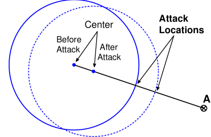
Figure 2: Illustration of a poisoning attack. By iteratively inserting malicious training points an attacker can gradually corrupt “drag” the centroid into a direction of an attack.

What points should be used by an attacker in order to subvert online anomaly detection? Intuitively one can expect that the optimal one-step displacement of the center of mass is achieved by placing attack point $\mathbf{x}_{i}$ at the line connecting $\mathbf{c}$ and $\mathbf{A}$ such that $||\mathbf{x}_{i}-\mathbf{c}||=r$. A formal proof of the optimality of such strategy and estimation of its efficiency constitutes the main objective of security analysis of online anomaly detection.

In order to quantify the effectiveness of a poisoning attack, we define the $i$-th relative displacement of the center of mass. This quantity measures the relative length of the projection of $\mathbf{c}_{i}$ onto the “attack direction” $\mathbf{a}$ in terms of the radius of the normality ball.

Definition 1 (Relative displacement)

(a) Let $\mathbf{A}$ be an attack point and define by $\mathbf{a}=\frac{\mathbf{A}-\mathbf{c}_{0}}{||\mathbf{A}-\mathbf{c}_{0}||}$ the according attack direction vector. The $i$-th relative displacement, denoted by $D_{i}$, is defined as

$$D_{i}=\frac{(\mathbf{c}_{i}-\mathbf{c}_{0})\cdot\mathbf{a}}{r}$$

. W.l.o.g. we assume that $\mathbf{c}_{0}=\mathbf{0}$.

(b) Attack strategies maximizing the displacement $D_{i}$ in each iteration $i$ are referred to as greedy optimal attack strategies.

3 Attack Effectiveness for Infinite Horizon Centroid Learner

The effectiveness of a poisoning attack for an infinite horizon has been analyzed in Nelson and Joseph (2006). We provide an alternative proof that follows the framework proposed in the introduction.

Theorem 2

The $i$-th relative displacement $D_{i}$ of the online centroid learner with an infinite horizon under the poisoning attack is bounded by

$$D_{i}\leq\,{\rm ln}\left(1+\frac{i}{n}\right)~{},$$ (3)

where $i$ is the number of attack points and $n$ the number of initial training points.

Proof  We first determine an optimal attack strategy and then bound the attack progress.

(a) Let $\mathbf{A}$ be an attack point and denote by $\mathbf{a}$ the corresponding attack direction vector. Let $\{\mathbf{a}_{i}|i\in\mathbb{N}\}$ be adversarial training points. The center of mass at the $i$-the iteration is given in the following recursion:

$$\mathbf{c}_{i+1}=\left(1-\frac{1}{n+i}\right)\mathbf{c}_{i}+\frac{1}{n+i}\mathbf{a}_{i+1},$$ (4)

with initial value $\mathbf{c}_{0}=0$. By the construction of the poisoning attack, $||\mathbf{a}_{i}-\mathbf{c}_{i}||\leq r$, which is equivalent to $\mathbf{a}_{i}=\mathbf{c}_{i}+\mathbf{b}_{i}$ with $||\mathbf{b}_{i}||\leq r$. Eq. (4) can thus be transformed into

$$\mathbf{c}_{i+1}=\mathbf{c}_{i}+\frac{1}{n+i}\mathbf{b}_{i}.$$

Taking scalar product with $\mathbf{a}$ and using the definition of a relative displacement, we obtain:

$$D_{i+1}=D_{i}+\frac{1}{n+i}\cdot\frac{\mathbf{b}_{i}\cdot\mathbf{a}}{r},$$ (5)

with $D_{0}=0$. The right-hand side of the Eq. (5) is clearly maximized under $||\mathbf{b}_{i}||\leq 1$ by setting $\mathbf{b}_{i}=r\mathbf{a}$. Thus the optimal attack is defined by

$$\mathbf{a}_{i}=\mathbf{c}_{i}+r\mathbf{a}.$$ (6)

(b) Plugging the optimal strategy $\mathbf{b}_{i}=r\mathbf{a}$ into Eq (5), we have:

$$D_{i+1}=D_{i}+\frac{1}{n+i}.$$

This recursion can be explicitly solved, taking into account that $d_{0}=0$, resulting in:

$$D_{i}=\sum_{k=1}^{i}\frac{1}{n+k}=\sum_{k=1}^{n+i}\frac{1}{k}-\sum_{k=1}^{n}\frac{1}{k}~{}.$$

Inserting the upper bound on the harmonic series, $\sum_{k=1}^{m}\frac{1}{k}=\ln(m)+\epsilon_{m}$ with $\epsilon_{m}\geq 0$ into the above formula, and noting that $\epsilon_{m}$ is monotonically decreasing, we obtain

$$D_{i}\leq{\rm ln}(n+i)-{\rm ln}(n)={\rm ln}\left(\frac{n+i}{n}\right)={\rm ln}\left(1+\frac{i}{n}\right),$$

which completes the proof.  

Since the bound in Eq. (3) is monotonically increasing, we can invert it to obtain the estimate of the effort needed by an attacker to achieve his goal:

$$i\geq n\cdot\left(\exp\left(D^{*}\right)-1\right)~{}.$$

It can be seen that an effort need to poison a online centroid learner is exponential in terms of the relative displacement of the center of mass. In other words, an attacker’s effort grows prohibitively fast with respect to the separability of an attack from the innocuous data. However, this is not surprising since due the infinitely growing training window the contribution of new points to the computation of the center of mass is steadily decreasing.

4 Poisoning Attack against Finite Horizon Centroid Learner

As it was shown in Section 2.3, the poisoning attack is ineffective against online centroid anomaly detection if all points are kept “in memory”. Unfortunately, memorizing the points defeats the main purpose of online algorithms, i.e., their ability to adjust to non-stationarity. Hence it is important to understand how the removal of data points from a working set affects the security of online anomaly detection. For that, the specific removal strategies presented in Section 2.2 must be considered.

It will turn out that for the average- and random-out rules the analysis can be carried out theoretically. For the nearest-out rule the analysis is more complicated but an optimal attack can be stated as mathematical optimization problem, and the attack effectiveness can be analyzed empirically.

4.1 Poisoning Attack for Average- and Random-out Rules

We begin our analysis with the average-out learner which follows exactly the same update rule as the infinite-horizon online centroid learner with the exception that the window size $n$ remains fixed instead of growing indefinitely (cf. Section 2.2). Despite the similarity to the infinite-horizon case, the result presented in the following theorem is surprisingly pessimistic.

Theorem 3

The $i$-th relative displacement $D_{i}$ of the online centroid learner with the average-out update rule under an worst-case optimal poisoning attack is

$$D_{i}=\frac{i}{n},$$ (7)

where $i$ is the number of attack points and $n$ is the training window size.

Proof  The proof is similar to the proof of Theorem 2. By explicitly writing out the recurrence between subsequent displacements, we conclude that the optimal attack is also attained by placing an attack point on the line connecting $\mathbf{c}_{i}$ and $\mathbf{a}$ at the edge of the sphere (cf. Eq. (6)):

$$\mathbf{a}_{i}=\mathbf{c}_{i}+r\mathbf{a}.$$

It follows that the relative displacement under the optimal attack is

$$D_{i+1}=D_{i}+\frac{1}{n}.$$

Since this recurrence is independent of the running index $i$, the displacement is simply accumulated over each iteration, which yields the bound of the theorem.  

One can see, that unlike the logarithmic bound in Theorem 2, the average-out learner is characterized by a linear bound on the displacement. As a result, an attacker only needs a linear amount of injected points – instead of an exponential one – in order to subvert an average-out learner. This cannot be considered secure.

We obtain a similar result for the random-out removal strategy.

Theorem 4

For the $i$-th relative displacement $D_{i}$ of the online centroid learner with the random-out update rule under an worst-case optimal poisoning attack it holds

$$E(D_{i})=\frac{i}{n},$$ (8)

where $i$ is the number of attack points, $n$ is the training window size, and the expectation is drawn over the choice of the removed data points.

Proof  The proof is based on the observation that the random-out rule in expectation boils down to average-out, and hence is reminiscent to the proof of Th. 3.  

4.2 Poisoning Attack for Nearest-out Rule

Let us consider the alternative update strategies mentioned in Section 2.1. The update rule $\mathbf{c}^{\prime}=\mathbf{c}+\frac{1}{n}(\mathbf{x}-\mathbf{x}_{0})$ of the oldest-out strategy is essentially equivalent to the update rule of the average-out except that the outgoing center $\mathbf{c}$ is replaced by the oldest point $\mathbf{x}_{0}$. In both cases the point to be removed is fixed in advance regardless of an attacker’s moves, hence the pessimistic result developed in Section 4.1 remains valid for this case. On average, the random-out update strategy is – despite its nondeterministic nature – equivalent to the average-out strategy. Hence, it also cannot be considered secure against a poisoning attack.

One might expect that the nearest-out strategy poses a stronger challenge to an attacker, as it tries to keep as much of a working set diversity as possible by retaining the most similar data to a new point. It turns out, however, that even this strategy can be broken with a feasible amount of work if an attacker follows a greedy optimal strategy. The latter is a subject of our investigation in this section.

4.2.1 An optimal attack

Our investigation focuses on a greedy optimal attack, i.e., an attack that provides a maximal gain for an attacker in a single iteration. For the infinite-horizon learner (and hence also for the average-out learner, as it uses the same recurrence in a proof), it is possible to show that the optimal attack yields the maximum gain for the entire sequence of attack iterations. For the nearest-out learner, it is hard to analyze a full sequence of attack iterations, hence we limit our analysis to a single-iteration gain. Empirically, even a greedy optimal attack turns out to be effective.

To construct a greedy optimal attack, it suffices to determine for each point $\mathbf{x}_{i}$ the location of an optimal attack point $\mathbf{x}_{i}^{*}$ to replace $\mathbf{x}_{i}$. This can be formulated as the following optimization problem:

Optimization Problem 5 (greedy optimal attack)

$$\{\mathbf{x}_{i}^{*},f_{i}\}\;=\;\; \max_{\mathbf{x}}\;\; (\mathbf{x}-\mathbf{x}_{i})\cdot\mathbf{a}$$ (9.a)

s.t. $$\|\mathbf{x}-\mathbf{x}_{i}\|\leq\|\mathbf{x}-\mathbf{x}_{j}\|,\quad\forall j=1,...,n$$ (9.b)

$$\|\mathbf{x}-\textstyle\frac{1}{n}\sum_{j=1}^{n}\mathbf{x}_{j}\|\leq r.$$ (9.c)

The objective of the optimization problem 5 reflects an attacker’s goal of maximizing the projection of $\mathbf{x}-\mathbf{x}_{i}$ onto the attack direction vector $\mathbf{a}$. The constraint (9.b) specifies the condition that the point $\mathbf{x}_{i}$ is the nearest neighbor of $\mathbf{x}$ (i.e., $\mathbf{x}$ falls into a Voronoi cell induced by $\mathbf{x}_{i}$). The constraint (9.c), when active, enforces that no solution lies outside of the sphere. Hence the geometric intuition behind an optimal attack, illustrated in Figure 3, is to replace some point with an attack point placed at the “corner” of the former’s Voronoi cell (including possibly a round boundary of the centroid) that provides a highest displacement of the center in the attack point’s direction.

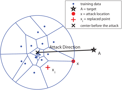
Figure 3: The geometry of a poisoning attack for the nearest-out rule. An optimal attack is achieved at the boundary of a Voronoi cell.

The maximization of Eq. (5) over all points in a current working set yields the index of the point to be replaced by an attacker:

$$\alpha=\text{argmax}\,_{i\in{1,...,n}}\;f_{i}$$ (10)

By plugging the definition of a Euclidean norm into the inner optimization problem (5) and multiplying out the quadratic constraints, all but one norm constraints reduce to simpler linear constraints:

$$\{\mathbf{x}_{i}^{*},f_{i}\}\;=\;\; \max_{\mathbf{x}}\;\; (\mathbf{x}-\mathbf{x}_{i})\cdot\mathbf{a}$$ (11.a)

s.t. $$2(\mathbf{x}_{j}-\mathbf{x}_{i})\cdot\mathbf{x}\leq\mathbf{x}_{j}\cdot\mathbf{x}_{j}-\mathbf{x}_{i}\cdot\mathbf{x}_{i},\quad\forall j=1,...,n$$ (11.b)

$$\mathbf{x}\cdot\mathbf{x}-\textstyle\frac{2}{n}\sum_{j=1}^{n}\mathbf{x}\cdot\mathbf{x}_{j}\leq r^{2}-\textstyle\frac{1}{n^{2}}\sum_{j,k=1}^{n}\mathbf{x}_{j}\cdot\mathbf{x}_{k}.$$ (11.c)

Due to the quadratic constraint (11.c), the inner optimization task is not as simple as a linear or a quadratic program. However, several standard optimization packages, e.g., CPLEX or MOSEK, can handle such so-called quadratically constrained linear programs (QCLP) rather efficiently, especially when there is only one quadratic constraint. Alternatively, one can use specialized algorithms for linear programming with a single quadratic constraint (van de Panne, 1966; Martein and Schaible, 2005) or convert the quadratic constraint to a second-order cone (SOC) constraint and use general-purpose conic optimization methods.

4.2.2 Implementation of a greedy optimal attack

Some additional work is needed for a practical implementation of a greedy optimal attack against a nearest-out learner.

A point can become “immune” to a poisoning attack, if its Voronoi cell does not overlap with the hypersphere of radius $r$ centered at $\mathbf{c}_{k}$, at some iteration $k$. The quadratic constraint (9.c) is never satisfied in this case, and the inner optimization problem (5) becomes infeasible. From then on, a point remains in the working set forever and slows down the attack progress. To avoid this awkward situation, an attacker must keep track of all optimal solutions $\mathbf{x}_{i}^{*}$ of the inner optimization problems. If any $\mathbf{x}_{i}^{*}$ slips out of the hypersphere after replacing the point $\mathbf{x}_{\alpha}$ with $\mathbf{x}_{\alpha}^{*}$, an attacker should ignore the outer loop decision (10) and instead replace $\mathbf{x}_{i}$ with $\mathbf{x}_{i}^{*}$.

A significant speedup can be attained by avoiding the solution of unnecessary QCLP problems. Let $S=\{1,\ldots,i-1\}$ and $\alpha_{S}$ be the current best solution of the outer loop problem (10) over the set $S$. Let $f_{\alpha_{S}}$ be the corresponding objective value of an inner optimization problem (3). Consider the following auxiliary quadratic program (QP):

$$\text{max}_{\mathbf{x}}\;\; \|\mathbf{x}-\textstyle\frac{1}{n}\sum_{j=1}^{n}\mathbf{x}_{j}\|$$ (12.a)

s.t. $$2(\mathbf{x}_{j}-\mathbf{x}_{i})\cdot\mathbf{x}\leq\mathbf{x}_{j}\cdot\mathbf{x}_{j}-\mathbf{x}_{i}\cdot\mathbf{x}_{i},\quad\forall j=1,...,n$$ (12.b)

$$(\mathbf{x}-\mathbf{x}_{i})\cdot\mathbf{a}\geq f_{\alpha_{S}}.$$ (12.c)

Its feasible set comprises the Voronoi cell of $\mathbf{x}_{i}$, defined by constraints (12.b), further reduced by constraint (12.c) to the points that improve the current value $f_{\alpha_{S}}$ of the global objective function. If the objective function value provided by the solution of the auxiliary QP (4.2.2) exceeds $r$ then the solution of the local QCLP (3) does not provide an improvement of the global objective function $f_{\alpha_{S}}$. Hence an expensive QCLP optimization can be skipped.

4.2.3 Attack Effectiveness

To evaluate the effectiveness of a greedy optimal attack, we perform a simulation on an artificial geometric data. The goal of this simulation is investigate the behavior of the relative displacement $D_{i}$ during the progress of a greedy optimal attack.

An initial working set of size $n=100$ is sampled from a $d$-dimensional Gaussian distribution with unit covariance (experiments are repeated for various values of $d\in\{2,...,100\}$). The radius $r$ of the online centroid learner is chosen such that the expected false positive rate is bounded by $\alpha=0.001$. An attack direction $\mathbf{a}$, $\|\mathbf{a}\|=1$ is chosen randomly, and 500 attack iterations ($5*n$) are generated using the procedure presented in Sections 4.2.1 – 4.2.2. The relative displacement of the center in the direction of attack is measured at each iteration. For statistical significance, the results are averaged over $10$ runs.

Figure 4 shows the observed progress of the greedy optimal attack against the nearest-out learner and compares it to the behavior of the theoretical bounds for the infinite-horizon learner (the bound of Nelson et al.) and the average-out learner. The attack effectiveness is measured for all three cases by the relative displacement as a function of the number of iterations. Plots for the nearest-out learner are presented for various dimensions $d$ of the artificial problems tested in simulations. The following two observations can be made from the plots provided in Figure 4:

Firstly, the attack progress, i.e., the functional dependence of the relative displacement of the greedy optimal attack against the nearest-out learner with respect to the number of iterations, is linear. Hence, contrary to the initial intuition, the removal of nearest neighbors to incoming points does not add security against a poisoning attack.

Secondly, the slope of the linear attack progress increases with the dimensionality of the problem. For low dimensionality, the relative displacement of the nearest-out learner is comparable, in absolute terms, with that of the infinite-horizon learner. For high dimensionality, the nearest-out learner becomes even less secure than the simple average-out learner. By increasing the dimensionality beyond $d>n$ the attack effectiveness cannot be increased. Mathematical reasons for such behavior are investigated in Section B.1.

A further illustration of the behavior of the greedy optimal attack is given in Figure 4, showing the dependence of the average attack slope on the dimensionality. One can see that the attack slope increases logarithmically with the dimensionality and wanes out to a constant factor after the dimensionality exceeds the number of training data points. A theoretical explanation of the observed experimental results is given in the next section.

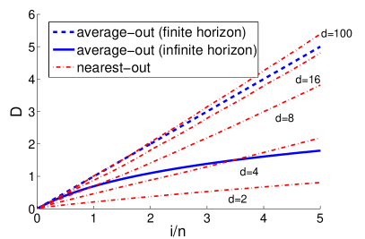
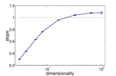
Figure 4: Effectiveness of a poisoning attack for the nearest-out rule as a function of input space dimensionality. The displacement of a centroid into a direction of an attack grows linearly with the number of injected points. The slope of the linear growth increases with the input space dimensionality. Upper bounds on the displacement of the average-out rule rule are plotted for comparison.

4.3 Concluding Remarks

To summarize our analysis for the case of attacker’s full control over the data, we conclude that an optimal poisoning attack can successfully subvert a finite-horizon online centroid learner for all outgoing point selection rules. This conclusion contrasts with the analysis of the infinite-horizon learner carried out in Barreno et al. (2006) that yields a logarithmic attack progress. As a compromise, one can in practice choose a large working set size $n$, which reduces the slope of a linear attack progress.

Among the different outgoing point selection rules, the nearest-out rule presents some challenges to the implementation of an optimal attack; however, some approximations can make such an attack feasible while still maintaining a reasonable progress rate. The key factor for the success of a poisoning attack in the nearest-out case lies in the high dimensionality of the feature space. The progress of an optimal poisoning attack depends on the size of Voronoi cells induced by the training data points. The size of Voronoi cells is related linearly to the volume of the sphere corresponding to attack’s feasible region. The increasing dimensionality of a feature space blows up the volume of the sphere and hence causes a higher attack progress rate.

In the following sections we analyze two additional factors that can affect the progress of a poisoning attack. First, we consider the case of an attacker being able to control only a fixed fraction $\nu$ of the training data. Subsequently we analyze a scenario in which an attacker is not allowed to exceed a certain false positive rate $\alpha$, e.g., by stopping online learning when a high false positive rate is observed. In will be shown that both of these possible constraints significantly reduce the effectiveness of a poisoning attack.

5 Poisoning Attack with Limited Bandwidth Constraint

We now proceed with investigation of a poisoning attack under a limited bandwidth constraint imposed on an attacker. We assume that an attacker can only inject up to a fraction of $\nu$ of the training data. In security applications, such an assumption is natural, as it may be difficult for an attacker to surpass a certain amount of innocuous traffic. For simplicity, we restrict ourselves to the average-out learner, as we have seen that it only differs by a constant from a nearest-out one and in expectation equals a random-out one.

5.1 Learning and Attack model

The initial online centroid learner is centered at the position $\mathbf{X}_{0}$ and has the radius $r$ (w.l.o.g. assume $X_{0}=0$ and $r=1$). At each iteration a new training point arrives which is either inserted by an adversary or is drawn independently from the distribution of innocuous points, and a new center of mass $\mathbf{X}_{i}$ is calculated. The mixing of innocuous and attack points is modeled by a Bernoulli random variable with the parameter $\nu$. Adversarial points $\mathbf{A}_{i}$ are chosen according to an attack function $f$ depending on the actual state of the learner $\mathbf{X}_{i}$. The innocuous pool is modeled by a probability distribution, from which the innocuous points ${\boldsymbol{\epsilon}}_{i}$ are independently drawn. We assume that the expectation of innocuous points ${\boldsymbol{\epsilon}}_{i}$ coincides with the initial center of mass: $E({\boldsymbol{\epsilon}}_{i})=\mathbf{X}_{0}$. Furthermore, we assume that all innocuous points are accepted by the initial learner, i.e., $\|{\boldsymbol{\epsilon}}_{i}-X_{0}\|\leq r$.

Moreover, for didactical reasons, we make a rather artificial assumption, which we will drop in the next chapter: all innocuous points are accepted by the learner, at any time of the attack, independent of their actual distance to the center of mass. In the next section we drop this assumption, such that the learner only accept points which fall within the actual radius.

The described probabilistic model is formalized by the following axiom.

Axiom 6

$\{B_{i}|i\in\mathbb{N}\}$ are independent Bernoulli random variables with parameter $\nu>0$. ${\boldsymbol{\epsilon}}_{i}$ are i.i.d. random variables in a reproducing kernel Hilbert space $\mathcal{H}$, drawn from a fixed but unknown distribution $P_{\boldsymbol{\epsilon}}$, satisfying $E({\boldsymbol{\epsilon}}_{i})=\mathbf{0}$ and $\|{\boldsymbol{\epsilon}}_{i}\|\leq r=1$ for each $i$. $B_{i}$ and ${\boldsymbol{\epsilon}}_{j}$ are mutually independent for each $i,j$. $f:\mathcal{H}\rightarrow\mathcal{H}$ is an attack strategy satisfying $\|f(x)-x\|\leq r$. $\{X_{i}|i\in\mathbb{N}\}$ is a collection of random vectors such that $\mathbf{X}_{0}=0$ and

$$\mathbf{X}_{i+1}=\mathbf{X}_{i}+\frac{1}{n}\left(B_{i}f(\mathbf{X}_{i})+(1-B_{i}){\boldsymbol{\epsilon}}_{i}-\mathbf{X}_{i}\right).$$ (13)

For simplicity of notation, we in this section refer to a collection of random vectors $\{\mathbf{X}_{i}|i\in\mathbb{N}\}$ satisfying Axiom 6 as online centroid learner denoted by $\mathcal{C}$. Furthermore we denote $\epsilon:={\boldsymbol{\epsilon}}\cdot\mathbf{a}$. Any function $f$ satisfying Ax. 6 is called attack strategy.

According to the above axiom an adversary’s attack strategy is formalized by an arbitrary function $f$. This raises the question which attack strategies are optimal in the sense that an attacker reaches his goal of concealing a predefined attack direction vector in a minimal number of iterations. An attack’s progress is measured by projecting the current center of mass onto the attack direction vector:

Definition 7

(a) Let $\mathbf{a}$ be an attack direction vector (w.l.o.g. $||\mathbf{a}||=1$), and let $\mathcal{C}=\{\mathbf{X}_{i}|i\in\mathbb{N}\}$ be a online centroid learner. The $i$-th displacement of $\mathcal{C}$, denoted by $D_{i}$, is defined by

$$D_{i}=\frac{X_{i}\cdot\mathbf{a}}{R}~{}.$$

(b) Attack strategies maximizing the displacement $D_{i}$ in each iteration $i$ are referred to as optimal attack strategies.

5.2 An Optimal Attack

The following result characterizes an optimal attack strategy for the model specified in Axiom 6.

Proposition 8

Let $\mathbf{a}$ be an attack direction vector and let $\mathcal{C}$ be a centroid learner. Then the optimal attack strategy $f$ is given by

$$f(X_{i}):=X_{i}+\mathbf{a}~{}.$$ (14)

Proof  Since by Axiom 6 we have $\|f(x)-x\|\leq r,$ any valid attack strategy can be written as $f(x)=x+g(x)$, such that $\|g\|\leq r=1.$ It follows that

$$\begin{split}D_{i+1}&\leq\mathbf{X}_{i+1}\cdot\mathbf{a}\\ &=\left(\mathbf{X}_{i}+\frac{1}{n}\left(B_{i}f(\mathbf{X}_{i})+(1-B_{i}){\boldsymbol{\epsilon}}_{i}-\mathbf{X}_{i}\right)\right)\cdot\mathbf{a}\\ &=D_{i}+\frac{1}{n}(B_{i}D_{i}+B_{i}g(\mathbf{X}_{i})\!\cdot\!\mathbf{a}+(1\!-\!B_{i})\epsilon_{i}-D_{i})\,.\end{split}$$

Since $B_{i}\geq 0$, the optimal attack strategy should maximize $g(\mathbf{X}_{i})\cdot\mathbf{a}$ subject to $||g(\mathbf{X}_{i})||\leq 1$. The maximum is clearly attained by setting $g(\mathbf{X}_{i})=\mathbf{a}$.  

5.3 Attack Effectiveness

The estimate of an optimal attack’s effectiveness in the limited control case is given in the following theorem.

Theorem 9

Let $\mathcal{C}$ be a centroid learner under an optimal poisoning attack. Then, for the displacement $D_{i}$ of $\mathcal{C}$, it holds:

$${\rm(a)}~{}~{}~{} E(D_{i}) =~{}(1-c_{i})\frac{\nu}{1-\nu}$$

$${\rm(b)}~{}~{}~{} {\rm Var}(D_{i}) \leq~{}\gamma_{i}\left(\frac{\nu}{1-\nu}\right)^{2}+\delta_{n}$$

where $\gamma_{i}=c_{i}-d_{i}$, $c_{i}:=\left(1-\frac{1-\nu}{n}\right)^{i}$, $d_{i}=\left(1-\frac{1-\nu}{n}\left(2-\frac{1}{n}\right)\right)^{i}$ and $\delta_{n}:=\frac{\nu^{2}+(1-d_{i})}{(2n-1)(1-\nu)^{2}}$.

Proof  (a) Inserting the optimal attack strategy of Eq. (14) into Eq. (13) of Ax. 6, we have:

$$\mathbf{X}_{i+1}=\mathbf{X}_{i}+\frac{1}{n}\left(B_{i}\left(\mathbf{X}_{i}+\mathbf{a}\right)+(1-B_{i}){\boldsymbol{\epsilon}}_{i}-\mathbf{X}_{i}\right)~{},$$

which can be rewritten as:

$$\mathbf{X}_{i+1}=\left(1-\frac{1-B_{i}}{n}\right)\mathbf{X}_{i}+\frac{B_{i}}{n}\mathbf{a}+\frac{(1-B_{i})}{n}{\boldsymbol{\epsilon}}_{i}~{}.$$ (15)

Taking the expectation on the latter equation, and noting that by Axiom 6 $E({\boldsymbol{\epsilon}})=0$ and $E(B_{i})=\nu$ holds, we have

$$E\left(\mathbf{X}_{i+1}\right)=\left(1-\frac{1-\nu}{n}\right)E(\mathbf{X}_{i})+\frac{\nu}{n}\mathbf{a}~{},$$

which by Def. 7 translates to

$$E(D_{i+1})=\left(1-\frac{1-\nu}{n}\right)E(D_{i})+\frac{\nu}{n}~{}.$$

The statement (a) follows from the latter recursive eequation by Prop. 17 (formula of the geometric series). For the more demanding proof of (b), see Appendix B.2.  

The following corollary shows the asymptotic behavior of the above theorem.

Corollary 10

Let $\mathcal{C}$ be a centroid learner satisfying under an optimal poisoning attack. Then. for the displacement $D_{i}$ of $\mathcal{C}$, it holds:

$${\rm(a)}\quad\quad E(D_{i}) \leq \frac{\nu}{1-\nu}~{}~{}\text{for all}~{}i$$

$${\rm(b)}\hskip 2.0pt\quad{\rm Var}(D_{i}) \rightarrow 0\quad\quad~{}~{}\text{for}~{}i,n\rightarrow\infty.$$

Proof  The corollary follows by   $\gamma_{i},\delta_{n}\rightarrow 0$   for $i,n\rightarrow\infty$.  

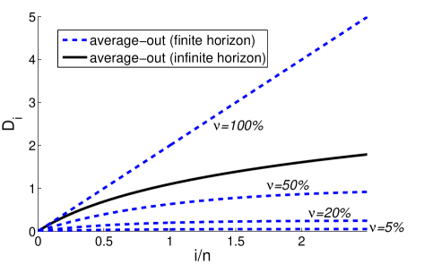
Figure 5: Theoretical behavior of the displacement of a centroid under a poisoning attack for a bounded fraction of traffic under attacker’s control. The infinite horizon bound of Nelson et al. is shown for comparison (solid line).

The growth of the above bounds as a function of an number of attack iterations is illustrated in Fig. 5. One can see that the attack’s success strongly depends on the fraction of the training data controlled by an attacker. For small $\nu$, the attack progress is bounded by a constant, which implies that an attack fails even with an infinite effort. This result provides a much stronger security guarantee than the exponential bound for the infinite horizon case.

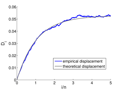
Figure 6: Comparison of empirical displacemend of the centroid under poisoning attack with attacker’s limited control ($\nu=0.05$) with a theoretical bound for the same setup. Emprical results are averaged over 10 runs; standard deviation is shown by vertical bars.

To empirically investigate the tightness of the derived bound we compute a Monte Carlo simulation of Axiom 6 with the parameters $\nu=0.05$, $n=100000$, $\mathcal{H}=\mathbb{R}^{2}$, and $\epsilon$ being a uniform distribution over the unit circle. Fig. 6 shows a typical displacement curve over the first $500,000$ attack iterations. Errorbars are computed over $10$ repetitions of the simulation.

6 Poisoning Attack under False Positive Constraints

In the last section we have assumed, that innocuous training points ${\boldsymbol{\epsilon}}_{i}$ are always accepted by the online centroid learner. But while an attacker displaces the hypersphere, it may happen that some innocuous points drop out of the hypersphere’s boundary. We have seen that an attacker’s impact highly depends on the fraction of points he places. If an attacker succeeds in pushing the hypersphere far enough such that sufficiently many innocuous points drop out, he can quickly displace the hypersphere.

6.1 Learning and Attack Model

Motivated by the above considerations we modify the probabilistic model of the last section as follows. Again we consider a online centroid learner initially anchored at a position $\mathbf{X}_{0}$ having a radius $r$, for the sake of simplicity and without loss of generality $\mathbf{X}_{0}=0$ and $r=1$. Then innocuous and adversarial points are mixed into the training data according to a fixed fraction, controlled by a binary valued random variable $B_{i}$. But now, in contrast to the last section, innocuous points ${\boldsymbol{\epsilon}}_{i}$ are only accepted if and only if they fall within a radius of $r$ of the hypersphere’s center $\mathbf{X}_{i}$. In addition, to avoid the learner being quickly displaced, we require that the false alarm rate is bounded by $\alpha$. If the latter is exceeded, we assume the adversary’s attack to have failed, i.e., a safe state of the learner is loaded and the online update mechanism is temporarily switched off.

We formalize the probabilistic model as follows:

Axiom 11

$\{B_{i}|i\in\mathbb{N}\}$ are independent Bernoulli random variables with parameter $\nu>0$. ${\boldsymbol{\epsilon}}_{i}$ are i.i.d. random variables in a reproducing kernel Hilbert space $\mathcal{H}$, drawn from a fixed but unknown distribution $P_{\boldsymbol{\epsilon}}=P_{-{\boldsymbol{\epsilon}}}$, satisfying $E({\boldsymbol{\epsilon}}_{i})=\mathbf{0}$, and $\|{\boldsymbol{\epsilon}}_{i}\|\leq r=1$ for each $i$. $B_{i}$ and ${\boldsymbol{\epsilon}}_{j}$ are mutually independent for each $i,j$. $f:\mathcal{H}\rightarrow\mathcal{H}$ is an attack strategy satisfying $\|f(x)-x\|\leq r$. $\{X_{i}|i\in\mathbb{N}\}$ is a collection of random vectors such that $\mathbf{X}_{0}=\mathbf{0}$ and

$$\mathbf{X}_{i+1}=\mathbf{X}_{i}+\frac{1}{n}\left(B_{i}\left(f(\mathbf{X}_{i})-\mathbf{X}_{i}\right)+(1-B_{i})I_{\{\|{\boldsymbol{\epsilon}}_{i}-\mathbf{X}_{i}\|\leq r\}}\left({\boldsymbol{\epsilon}}_{i}-\mathbf{X}_{i}\right)\right)~{},$$ (16)

if $E_{{\boldsymbol{\epsilon}}_{i}}\left(I_{\{\|{\boldsymbol{\epsilon}}_{i}-\mathbf{X}_{i}\|\leq r\}}\right)\leq 1-\alpha$ and by $\mathbf{X}_{i+1}=\mathbf{0}$ elsewise.

For simplicity of notation, we in this section refer to a collection of random vectors $\{\mathbf{X}_{i}|i\in\mathbb{N}\}$ satisfying Ax. 11 as online centroid learner with maximal false positive rate $\alpha$ denoted by $\mathcal{C}$. Any function $f$ satisfying Ax. 11 is called attack strategy. Optimal attack strategies are characterized in term of the displacement as in the previous section (see Def. 7).

6.2 Optimal Attack and Attack Effectiveness

The following result characterizes an optimal attack strategy for the model specified in Axiom 11.

Proposition 12

Let $\mathbf{a}$ be an attack direction vector and let $\mathcal{C}$ be a centroid learner with maximal false positive rate $\alpha$. Then an optimal attack strategy $f$ is given by

$$f(X_{i}):=X_{i}+\mathbf{a}~{}.$$

Proof  Since by Axiom 11 we have $\|f(x)-x\|\leq r,$ any valid attack strategy can be written as $f(x)=x+g(x)$, such that $\|g\|\leq r=1.$ It follows that either $D_{i}=0$, in which case the optimal $f$ is arbitrary, or we have

$$D_{i+1} = \mathbf{X}_{i+1}\cdot\mathbf{a}$$

$$= \left(\mathbf{X}_{i}+\frac{1}{n}\left(B_{i}f(\mathbf{X}_{i})+(1-B_{i}){\boldsymbol{\epsilon}}_{i}-\mathbf{X}_{i}\right)\right)\cdot\mathbf{a}$$

$$= D_{i}+\frac{1}{n}\left(B_{i}\left(D_{i}+g(\mathbf{X}_{i})\right)+(1-B_{i}){\boldsymbol{\epsilon}}_{i}-D_{i}\right)$$

Since $B_{i}\geq 0$, the optimal attack strategy should maximize $g(\mathbf{X}_{i})\cdot\mathbf{a}$ subject to $||g(\mathbf{X}_{i})||\leq 1$. The maximum is clearly attained by setting $g(\mathbf{X}_{i})=\mathbf{a}$.  

The estimate of an optimal attack’s effectiveness in the limited control case is given in the following main theorem of this paper.

Theorem 13

Let $\mathcal{C}$ be a centroid learner with maximal false positive rate $\alpha$ under a poisoning attack. Then, for the displacement $D_{i}$ of $\mathcal{C}$, it holds:

$${\rm(a)}~{}~{}~{} E(D_{i}) \leq(1-c_{i})\frac{\nu+\alpha(1-\nu)}{(1-\nu)(1-\alpha)}$$

$${\rm(b)}~{}~{}~{} {\rm Var}(D_{i}) \leq\gamma_{i}\frac{\nu^{2}}{(1-\alpha)^{2}(1-\nu)^{2}}+\rho(\alpha)+\delta_{n}$$

where $c_{i}:=\left(1-\frac{(1-\nu)(1-\alpha)}{n}\right)^{i}$,   $d_{i}=\left(1-\frac{1-\nu}{n}(2-\frac{1}{n})(1-\alpha)\right)^{i}$,   $\gamma_{i}=(c_{i}-d_{i})$,   $\rho(\alpha)=\alpha\frac{(1-c_{i})(1-d_{i})(2\nu(1-\alpha)+\alpha)}{(1-\frac{1}{2n})(1-\nu)^{2}(1-\alpha)^{2}}$,   and $\delta_{n}=\frac{(1-d_{i})(\nu+(1-\nu)E(\epsilon_{i}^{2}))}{(2n-1)(1-\nu)(1-\alpha)}$.

The proof is technically demanding and is given in App. B.3. Despite the more general proof reasoning, we recover the tightness of the bounds of the previous section for the special case of $\alpha=0$, as shown by the following corollary.

Corollary 14

Suppose a maximal false positive rate of $\alpha=0$. Then, the bounds on the expected displacement $D_{i}$, as given by Th. 9 and Th. 13, coincident. Furthermore, the variance bound of Th. 13 upper bounds the one of Th. 9.

Proof  We start by setting $\alpha=0$ in Th. 13(a). Then, clearly the latter bound coincidents with its counterpart in Th. 9. For the proof of the second part of the corollary, we observe that $\rho(\alpha)=0$ and that the quantities $c_{i},d_{i},$ and $\gamma_{i}$ coincident with its counterparts in Th. 9. Moreover, removing the distribution dependence by upper bounding $E(\epsilon_{i})\leq 1$ reveals that $\delta_{i}$ is upper bounded by its counter part of Th. 9. Hence, the whole expression on the right hand side of Th. 13(b) is upper bounded by its counterpart in Th. 9(b).  

The following corollary shows the asymptotic behavior of the above theorem. It follows from $\gamma_{i},\delta_{n},\rho(\alpha)\rightarrow 0$ for $i,n\rightarrow\infty$, and $\alpha\rightarrow 0$, respectively.

Corollary 15

Let $\mathcal{C}$ be a centroid learner with maximal false positive rate $\alpha$ satisfying the optimal attack strategy. Then for the displacement of $\mathcal{C}$, denoted by $D_{i}$, we have:

$${\rm(a)}~{}~{}~{} E(D_{i}) \leq~{}~{}\frac{\nu+\alpha(1-\nu)}{(1-\nu)(1-\alpha)}~{}~{}~{}~{}~{}~{}~{}~{}~{}~{}\text{for all}~{}i\hskip 108.12054pt$$

$${\rm(b)}~{}~{}~{} {\rm Var}(D_{i}) \rightarrow~{}0\quad\quad\quad\quad\quad\quad\quad\quad\quad~{}\text{for}~{}i,n\rightarrow\infty,\alpha\rightarrow 0~{}.$$

From the previous theorem, we can see that for small false positive rates $\alpha\approx 0$, which are common in many applications, e.g., Intrusion Detection (see Sect. 7 for an extensive analysis), the bound approximately equals the one of the previous section, i.e., we have $E(D_{i})\leq\frac{\nu}{1-\nu}+\delta$ where $\delta>0$ is a small constant with $\delta\rightarrow 0$. Inverting the bound we obtain the useful formula

$$\nu\geq\frac{E(D_{i})}{1+E(D_{i})}$$ (17)

which gives a lower bound on the minimal $\nu$ an adversary has to employ for an attack to succeed.

The bound of Th. 13 is shown in Fig. 5 for different levels of false positive protection $\alpha\in[0,0.025]$. We are especially interested in low positive rates which are common in anomaly detection applications. One can see that much of the tightness of the bounds of the previous section is preserved. In the extreme case $\alpha=0$ the bounds coincident, as been shown in Cor. 14.

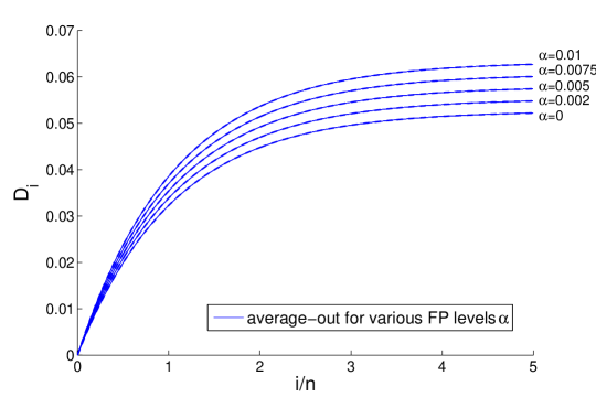
Figure 7: Theoretical behavior of the displacement of a centroid under a poisoning attack for different levels of false positive protection $\alpha$. The predicted displacement curve for $\alpha=0$ coincides with the one shown in Fig. 6.

7 Case Study: Application to Intrusion Detection

In this section we present the experimental evaluation of the developed analytical instruments in the context of a particular computer security application: intrusion detection. Centroid anomaly detection has been previously used in several intrusion detection systems (e.g., Hofmeyr et al., 1998; Lazarevic et al., 2003; Wang and Stolfo, 2004; Laskov et al., 2004b; Wang et al., 2005; Rieck and Laskov, 2006; Wang et al., 2006; Rieck and Laskov, 2007). After a short presentation of data collection, preprocessing and model selection, our experiments aim at verification of the theoretically obtained growth rates for attack progress as well as computation of constant factors for specific exploits.

7.1 Data Corpus and Preprocessing

The data to be used in our case study represents real HTTP traffic recorded at Fraunhofer FIRST. We consider the intermediate granularity level of requests which are the basic application-layer syntactic elements of the HTTP protocol. Packet headers have been stripped, and requests spread across multiple packets have been merged together. The resulting benign dataset consists of 2950 byte strings containing payloads of inbound HTTP requests. The malicious dataset consists of 69 attack instances from 20 classes generated using the Metasploit penetration testing framework. All exploits were normalized to match the frequent attributes of innocuous HTTP requests such that the malicious payload provides the only indicator for identifying the attacks.

As byte sequences are not directly suitable for application of machine learning algorithms, we deploy a $k$-gram spectrum kernel (Leslie et al., 2002; Shawe-Taylor and Cristianini, 2004) for the computation of the inner products. To enable fast comparison of large byte sequences (a typical sequence length 500-1000 bytes), efficient algorithms using sorted arrays (Rieck and Laskov, 2008) have been implemented. Furthermore, kernel values are normalized according to

$$k(\mathbf{x},\bar{\mathbf{x}})\longmapsto\frac{k(\mathbf{x},\bar{\mathbf{x}})}{\sqrt{k(\mathbf{x},\mathbf{x})k(\bar{\mathbf{x}},\bar{\mathbf{x}})}}~{},$$ (18)

to avoid a dependence on the length of a request payload. The resulting inner products subsequently have been processed by an RBF kernel.

7.2 Learning Model

The feature space selected for our experiments depends on two parameters: the $k$-gram length and the RBF kernel width $\sigma$. Prior to the main experiments aimed at the validation of proposed security analysis techniques, we investigate optimal model parameters in our feature space. The parameter range considered is $k=1,2,3$ and $\sigma=2^{-5},2^{-4},...,2^{5}$.

To carry out model selection, we randomly partitioned the innocuous corpus into disjoint training, validation and test sets (of sizes $1000$, $500$ and $500$). The training partition is comprised of the innocuous data only, as the online centroid learner assumes clean training data. The validation and test partitions are mixed with $10$ attack instances randomly chosen from different attack classes. For each partition, different online centroid learner models are trained on a training set and evaluated on a validation and a test sets using the normalized AUC_[0,0.01] as a performance measure. For statistical significance, model selection is repeated $1000$ times with different randomly drawn partitions. The average values of the normalized AUC_[0,0.01] for the different $k$ values on test partitions are given in Table 1.

It can be seen that the $3$-gram model consistently shows better AUC values for both the linear and the best RBF kernels. We have chosen the linear kernel for the remaining experiments, since it allows to carry out computations directly in input space with only a marginal penalty in detection accuracy.

	linear	best RBF kernel	optimal $\sigma$
1-grams	$0.913\pm 0.051$	$0.985\pm 0.021$	$2^{-2.5}$
2-grams	$0.979\pm 0.026$	$0.985\pm 0.025$	$2^{-1.5}$
3-grams	$0.987\pm 0.018$	$0.989\pm 0.017$	$2^{-0.5}$

Table 1: Accuracy of the linear kernel and the best RBF kernel as well as the optimal bandwidth $\sigma$.

7.3 Intrinsic HTTP Data Dimensionality

Dimensionality of training data makes an important contribution to the (in)security of the online centroid learner when using the nearest-out update rule. Simulations on artificial data (cf. Section 4.2.3) show that the slope of a linear progress rate of a poisoning attack increases for larger dimensionalities $d$. This can be also explained theoretically (cf. Section B.1) by the fact that radius of Voronoi cells induced by training data is proportional to $\sqrt[d]{1/n}$, which increases with growing $d$.

For the intrusion detection application at hand, the dimensionality of the chosen feature space ($k$-grams with $k=3$) is $256^{3}$. In view of Th. 16, the dimensionality of the relevant subspace in which attack takes place is bounded by the size of the training data $n$, which is much smaller, in the range of 100 – 1000 for realistic applications. Yet the real progress rate depends on the intrinsic dimensionality of the data. When the latter is smaller than the size of the training data, an attacker can compute a PCA of the data matrix (Schölkopf et al., 1998) and project the original data into a subspace spanned by a smaller number of informative components.

To determine the intrinsic dimensionality of possible training sets drawn from HTTP traffic, we randomly drew $1000$ elements from the training set, calculate a linear kernel matrix in the space of $3$-grams and compute its eigenvalue decomposition. We then determine the number of leading eigen-components preserving as a function of the percentage of variance preserved. The results averaged over 100 repetitions are shown in Fig. 8.

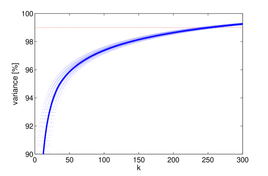
Figure 8: Intrinsic dimensionality of the embedded HTTP data. The preserved variance is plotted as a function of the number of eigencomponents, $k$, employed for calculation of variance (solid blue line). The tube indicates standard deviations.

It can be seen that $250$ kernel PCA components are needed to preserve 99% of the variance. This implies that, although effective dimensionality of HTTP traffic is significantly smaller that the number of training data points, it still remains sufficiently high so that the rate of attack progress approaches 1, which is similar to the simple average-out learner.

7.4 Geometrical Constraints of HTTP Data

Several technical difficulties arising from data geometry have to be overcome in launching a poisoning attack in practice. It turns out, however, that the consideration of the training data geometry provides an attacker with efficient tools for finding reasonable approximations for the above mentioned tasks.

(1) First, we cannot directly simulate a poisoning attack in the $3$-gram input space due to its high dimensionality. An approximately equivalent explicit feature space can be constructed by applying kernel PCA to the kernel matrix $K$. By pruning the eigenvalues “responsible” for dimensions with low variance one can reduce the size of the feature space to the implicit dimensionality of a problem if the kernel matches the data (Braun et al., 2008). In all subsequent experiments we used $d=256$ as suggested by the experiments in Section 7.3.

(2) Second the crucial normalization condition (18) requires that a solution lies on a unit sphere. Unfortunately, this renders the calculation of an optimal attack point non-convex. Therefore we pursue the following heuristic procedure to enforce normalization: we explicitly project local solutions (for each Voronoi cell) to a unit sphere, verify their feasibility (the radius and the cell constraints), and remove infeasible points from the outer loop (10).

(3) In general one cannot expect each feature space vector to correspond to a valid byte sequence since not all combinations of $k$-grams can be “glued” to a valid byte sequence. In fact, finding a sequence with the best approximation to a given $k$-gram feature vector has been shown to be NP-hard (Fogla and Lee, 2006). Fortunately by the fact that an optimal attack lies in the span of training data, i.e. Th. 16, we construct an attack’s byte sequence by concatenating original sequences of basis points with rational coefficients that approximately match the coefficients of the linear combination. A potential disadvantage of this method is the large increase in the sequence lengths. Large requests are conspicuous and may consume significant resources on the attacker’s part.

(4) An attack byte sequence must be embedded in a valid HTML protocol frame. Building a valid HTTP request with arbitrary content is, in general, a non-trivial task, especially if it is required that a request does not cause an error on a server. An HTTP request consists of fixed format headers and a variable format body. A most straightforward way to stealthily introduce arbitrary content is to provide a body in a request whose method (e.g., GET) does not require one. According to an RFC specification of the HTTP protocol, a request body should be ignored by a server in this case.

7.5 Poisoning Attack for Finite Horizon Centroid Learner

The analysis carried out in Section 4 shows that an online centroid learner, in general, does not provide sufficient security if an attacker fully controls the data. Practical efficiency of a poisoning attack, however, depends on the dimensionality and geometry of training data analyzed in the previous section. Theoretical results have been illustrated in simulations on artificial data presented in Section 4.2.3. Experiments in this section are intended to verify whether these findings hold for real attacks against HTTP applications. Our experiments focus on the nearest-out learner, as other update rules can be easily attacked with trivial methods.

We are now in the position to evaluate the progress rate of a poisoning attack on real network traffic and exploits. The goal of these experiments is to verify simulations carried out in Section 4.2.2 on real data.

Our experimental protocol is as follows. We randomly draw $n=250$ training points from the innocuous corpus, calculate the center of mass and fix the radius such that the false positive rate on the training data is $\alpha=0.001$. Then we draw a random instance from each of the 20 attack classes, and for each of these 20 attack instances generate a poisoning attack as described in Section 7.4. An attack succeeds when the attack point is accepted as innocuous by a learning algorithm.

For each attack instance, the number of iterations needed for an attack to succeed and the respective displacement of the center of mass is recorded. Figure 9 shows, for each attack instance, the behavior of the relative displacement at the point of success as a function of a number of iterations. We interpolate a “displacement curve” from these pointwise values by a linear least-squares regression. For comparison, the theoretical upper bounds for the average-out and all-in cases are shown. Notice that the bound for the all-in strategy is also almost linear for the small $i/n$ ratios observed in this experiment.

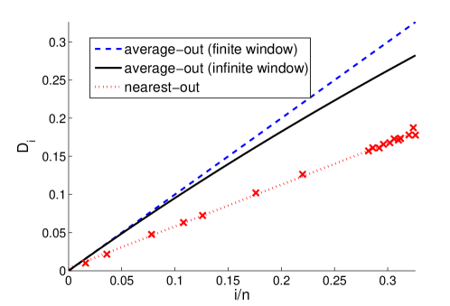
Figure 9: Empirical displacement of the nearest-out centroid for $20$ different exploits (crosses, linear fit shown by a red dotted line). Displacement values are shown at the point of success for each attack. Theoretical bounds are shown for comparison (blue and black lines).

The observed results confirm that the linear progress rate in the full control scenario can be attained in practice for real data. Compared to the simulations of Section 7.4, the progress rate of an attack is approximately half the one for the average-out case. Although this somewhat contradicts our expectation that for a high-dimensional space (of the effective dimensionality $d\sim 256$ as it was found in Section 7.3) the progress rate to the average-out case should be observed, this can be attributed to multiple approximations performed in the generation of an attack for real byte sequences. The practicality of a poisoning attack is further emphasized by a small number of iterations needed for an attack to succeed: from 0 to only 35 percent of the initial number of points in the training data have to be overwritten by an attacker.

7.6 Critical Traffic Ratios of HTTP Attacks

For the case of attacker’s limited control, the success of the poisoning attack largely depends on attacker’s constraints, as shown in the analysis in Sections 5 and 6. The main goal of the experiments in this section is therefore to investigate the impact of potential constraints in practice. In particular, we are interested in the impact of the traffic ratio $\nu$ and the false positive rate $\alpha$.

The analysis in Section 5 (cf. Theorem 9 and Figure 5) shows that the displacement of a poisoning attack is bounded from above by a constant, depending on the traffic ratio $\nu$ controlled by an attacker. Hence the susceptibility of a learner to a particular attack depends on the value of this constant. If an attacker does not control a sufficiently large traffic portion and the potential displacement is bounded by a constant smaller than the distance from the initial center of mass to the attack point, then an attack is bound to fail. To illustrate this observation, we compute critical traffic rates needed for the success of each of the 20 attack classes in our malicious pool.

We randomly draw a $1000$-elemental training set from the innocuous pool and calculate its center of mass (in the space of 3-grams). The radius is fixed such the false positive rate $\alpha=0.001$ on innocuous data is attained. For each of the 20 attack classes we compute the class-wise median distance to the centroid’s boundary. Using these distance values we calculate the “critical value” $\nu_{\text{crit}}$ by solving Th. 9(c) for $\nu$ (cf. Eq. (17)). The experiments have been repeated $10$ times results are shown in Table 2.

Attacks	Rel. dist.	$\boldsymbol{\nu}_{\textbf{crit}}$
ALT-N WebAdmin Overflow	$0.058\pm 0.002$	$0.055\pm 0.002$
ApacheChunkedEncoding	$0.176\pm 0.002$	$0.150\pm 0.001$
AWStats ConfigDir Execution	$0.067\pm 0.002$	$0.063\pm 0.002$
Badblue Ext Overflow	$0.168\pm 0.002$	$0.144\pm 0.001$
Barracuda Image Execution	$0.073\pm 0.002$	$0.068\pm 0.002$
Edirectory Host	$0.153\pm 0.002$	$0.132\pm 0.001$
IAWebmail	$0.178\pm 0.002$	$0.151\pm 0.001$
IIS 5.0 IDQ exploit	$0.162\pm 0.002$	$0.140\pm 0.001$
Pajax Execute	$0.107\pm 0.002$	$0.097\pm 0.002$
PEERCAST URL	$0.163\pm 0.002$	$0.140\pm 0.001$
PHP Include	$0.097\pm 0.002$	$0.088\pm 0.002$
PHP vBulletin	$0.176\pm 0.002$	$0.150\pm 0.001$
PHP XML RPC	$0.172\pm 0.002$	$0.147\pm 0.001$
HTTP tunnel	$0.160\pm 0.002$	$0.138\pm 0.001$
IIS 4.0 HTR exploit	$0.176\pm 0.002$	$0.149\pm 0.002$
IIS 5.0 printer exploit	$0.161\pm 0.002$	$0.138\pm 0.001$
IIS unicode attack	$0.153\pm 0.002$	$0.133\pm 0.001$
IIS w3who exploit	$0.168\pm 0.002$	$0.144\pm 0.001$
IIS 5.0 WebDAV exploit	$0.179\pm 0.002$	$0.152\pm 0.001$
rproxy exploit	$0.155\pm 0.002$	$0.134\pm 0.001$

Table 2: Relative distances (in radii) of exploits to the boundary of a centroid enclosing all training points and critical values of parameter $\nu$.

The results indicate that in order to subvert a online centroid learner an attacker needs to control from 5 to 20 percent of traffic. This could be a significant limitation on highly visible sites. Note that an attacker usually aims at earning money by hacking computer systems. However generating competitive bandwidths at highly visible site is likely to drive the attacker’s cost to exorbitant numbers.

On the other hand, one can see that the traffic rate limiting alone cannot be seen as sufficient protection instrument due to its passive nature. In the following section we investigate a different protection scheme using both traffic ratio and the false positive rate control.

7.7 Poisoning Attack against Learner with False Positive Protection

The analysis in Section 5 (cf. Theorem 9 and Figure 5) shows that the displacement of a poisoning attack is bounded from above by a constant, depending on a traffic ratio $\nu$ and a maximal false positive rate $\alpha$. Hence a detection system can be protected by observing the system’s false positive rate and switching off the online updates if a defined threshold is exceeded.

7.7.1 Experiment 1: Practicability of False Positive Protection

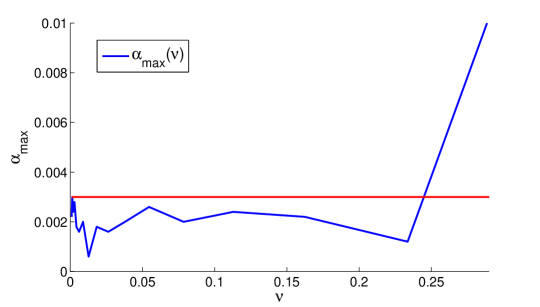
Figure 10: Maximal false positive rate within 10000 attack iterations as a function of $\nu$ (maximum taken over 10 runs).

However in practice the system should be as silent as possible, i.e., an administrator should be only alarmed if a fatal danger to the system is given. We hence in this section investigate how sensible the false positive rate is to small adversarial perturbations of the learner, caused by poisoning attack with small $\nu$.

Therefore the following experiment investigates the rise in the false positive rate $\alpha$ as a function of $\nu$. From the innocuous pool we randomly drew a $1000$-elemental training set on base of which a centroid is calculated. Thereby the radius is fixed to the empirical estimate of the $0.001$-quantile of the innocuous pool based on $100$ randomly drawn subsamples, i.e., we expect the centroid having a false positive rate of $\alpha=0.001$ on the innocuous pool. Moreover we randomly drew a second $500$-elemental training set from the innocuous pool which is reserved for online training and and a $500$-elemental hold out set on base of which a false positive rate can be estimated for a given centroid. Then we iteratively calculated poisoning attacks with fixed IIS 5.0 WebDAV exploit as attack point by subsequently presenting online training points to the centroid learner which are rejected or accepted based on whether they fall within the learner’s radius. For each run of a poisoning attack the false positiv rate is observed on base of the hold out set.

In Fig. 10 we plot for various values of $\nu$ the maximal observed false positive rate as a function of $\nu$, where the maximum is taken over all attack iterations and $10$ runs. One can see from the plot that $\alpha=0.005$ is a reasonable threshold in our setting to ensure the systems’s silentness.

7.7.2 Experiment 2: Attack Simulation for False Positive Protection

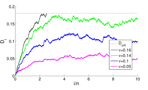
Figure 11: A simulation of a poisoning attack under limited control.

In the previous experiment we have seen that $\alpha=0.005$ is a reasonable threshold for a false positive protection to ensure a systems silentness. We in this section illustrate that the critical values from Section 7.6 computed on base of Th. 9 for maximal false positive rate of $\alpha=0.005$ still give a good approximation of the true impact of a poisoning attack.

We fix a particular exploit in our malicious corpus (IIS WebDAV 5.0 exploit) and run a poisoning attack against the average-out centroid for various values of $\nu\in[0.05,0.10,0.14,0.16]$, recording the actual displacement curves. One can see from Fig. 11 that the attack succeeds for $\nu=0.16$ but fails to reach the required relative displacement of $D_{crit}=0.18$ for $\nu=0.14$. The theoretically computed critical traffic ratio for this attack according to Table 2 is $\nu_{\rm crit}=0.152$. The experiment shows that the derived bounds are surprisingly tight in practice.

7.7.3 Implementation of Poisoning Protection

In Section 5 we have seen, that an attacker’s impact on corrupting the training data highly depends on the fraction of adversarial points in the training data stream. This implies that a high amount of innocuous training points constantly has to come in. In Section 6 we have seen, that we can secure the learner by setting a threshold on the false positive rate $\alpha$. Exceeding the latter enforces further defense processes such as switching off the online training process. Hence an confident estimation of $\alpha$ has to be at hand. How can we achieve the latter?

In practice, this can e.g. be done by caching the training data. When the cache exceeds a certain value at which we have a confident estimation of $\alpha$ (e.g., after 24 hours), the cached training data can be applied to the learner. Since in applications including intrusion detection, we usually deal with a very high amount of training data, a confident estimation is already possible after short time period.

8 Discussion and Conclusions

Understanding of security properties of learning algorithms is essential for their protection against abuse. The latter can take place when learning is used in applications with competitive interests at stake, e.g., security monitoring, games, spam protection, reputation systems, etc. Certain security properties of a learning algorithm must be proved in order to claim its immunity to abuse. To this end, we have developed a methodology for security analysis and applied it for a specific scenario of online centroid anomaly detection. The results of our analysis highlight conditions under which an attacker’s effort to subvert this algorithm is prohibitively high.

Several issues discussed in this contribution have appeared in related work albeit not in the area of anomaly detection. Perhaps the most consummate treatment of learning under an adversarial impact has been carried out by Dalvi et al. (2004). In this work, Bayesian classification is analyzed for robustness against adversarial impact. The choice of their classifier is motivated by widespread application of the naive Bayes classification in the domain of spam detection where real examples of adversarial impact have been observed for a long time. The adversarial classification is considered as a game between an attacker and a learner. Due to the complexity of analysis, only one move by each party can be analyzed. Similar to our approach, Dalvi et al. (2004) formalize the problem by defining cost functions of an attacker and a learner (Step 1) and determine an optimal adversarial strategy (Step 3). Although the attacker’s constraints are not explicitly treated theoretically, several scenarios using specific constraints have been tested experimentally. No analysis of the attacker’s gain is carried out; instead, the learner’s direct response to adversarial impact is considered.

A somewhat related approach has been developed for handling worst-case random noise, e.g., random feature deletion (Globerson and Roweis, 2006; Dekel and Shamir, 2008). Similar to Dalvi et al. (2004), both of these methods construct a classifier that automatically reacts to the worst-case noise or, equivalently, the optimal adversarial strategy. In both methods, the learning problem is formulated as a large-margin classification using a specially constructed risk function. An important role in this approach is played by the consideration of constraints (Step 2), e.g., in the form of the maximal number of corruptible features. Although these approaches do not quantitatively analyze attacker’s gain, (Dekel and Shamir, 2008) contains an interesting learning-theoretic argument that relates classification accuracy, sparseness, and robustness against adversarial noise.

To summarize, we believe that despite recent evidence of possible attacks against machine learning and the currently lacking theoretical foundations for learning under adversarial impact, machine learning algorithms can be protected against such impact. The key to such protection lies in quantitative analysis of security of machine learning. We have shown that such analysis can be rigorously carried out for specific algorithms and attacks. Further work should extend such analysis to more complex learning algorithms and a wider attack spectrum.

Acknowledgments

The authors wish to thank Ulf Brefeld, Konrad Rieck, Vojtech Franc, Peter Bartlett and Klaus-Robert Müller for fruitful discussions and helpful comments. Furthermore we thank Konrad Rieck for providing the network traffic. This work was supported in part by the German Bundesministerium für Bildung und Forschung (BMBF) under the project REMIND (FKZ 01-IS07007A), by the German Academic Exchange Service, and by the FP7-ICT Programme of the European Community, under the PASCAL2 Network of Excellence, ICT-216886.

A Notation Summary

In this paper we use the following notational conventions.

$\mathcal{C},r,\mathbf{c}$	centroid $\mathcal{C}$ with radius $r$ and center $\mathbf{c}$
$i$	$i$-th attack iteration, $i\in\mathbb{N}_{0}$
$\mathbf{x}_{i},\mathbf{X}_{i}$	center of centroid in $i$-th attack iteration
$\mathbf{A}$	attack point
$\mathbf{a}$	attack direction vector

$D_{i}$	$i$-th relative displacement of a centroid in radii into direction of $\mathbf{a}$
$n$	number of training patterns of centroid
$f$	function of $\mathcal{H}\rightarrow\mathcal{H}$ giving an attack strategy
$\nu$	fraction of adversarial training points
$B_{i}$	Bernoulli variable
$\epsilon_{i},{\boldsymbol{\epsilon}}_{i}$	i.i.d. noise
$\alpha$	false alarm rate
$I_{S}$	indicator function of a set $S$

B Auxiliary Material and Proofs

B.1 Auxiliary Material for Section 4

B.1.1 Representer Theorem for Optimal Greedy Attack

First, we show why the attack efficiency cannot be increased beyond dimensions with $d\geq n+1$. This follows from the fact that the optimal attack lies in the span of the working set points and the attack vector. The following representer theorem allows for “kernelization” of the optimal greedy attack.

Theorem 16

There exists an optimal solution of problem (3) satisfying

$$\mathbf{x}^{*}_{i}\in~{}{\rm span}(\mathbf{a},\mathbf{x}_{1},...,\mathbf{x}_{n}).$$ (19)

Proof  The Lagrangian of optimization problem (3) is given by:

$$L(\mathbf{x},{\boldsymbol{\alpha}},\beta) = -(\mathbf{x}-\mathbf{x}_{i})\cdot\mathbf{a}+\sum_{j=1}^{n}\alpha_{j}\left(2(\mathbf{x}_{j}-\mathbf{x}_{i})\cdot\mathbf{x}-\mathbf{x}_{j}\cdot\mathbf{x}_{j}+\mathbf{x}_{i}\cdot\mathbf{x}_{i}\right)$$

$$+\beta\left(\mathbf{x}\cdot\mathbf{x}-\frac{2}{n}\sum_{j=1}^{n}\mathbf{x}\cdot\mathbf{x}_{j}+\frac{1}{n^{2}}\sum_{j,k=1}^{n}\mathbf{x}_{j}\cdot\mathbf{x}_{k}-r^{2}\right)$$

Since the feasible set of problem (3) is bounded by the spherical constraint and is not empty ($\mathbf{x}_{i}$ trivially is contained in the feasible set), there exists at least one optimal solution $\mathbf{x}_{i}^{*}$ to the primal. For optimal $\mathbf{x}_{i}^{*}$, $\alpha^{*}$ and $\beta^{*}$, we have the following first order optimality conditions

$$\frac{\delta L}{\delta\mathbf{x}}=0:~{}~{}~{}~{}-\mathbf{a}-\frac{1}{n}\sum_{j=1}^{n}\mathbf{x}_{j}+2\sum_{j=1}^{n}\alpha_{j}^{*}(\mathbf{x}_{j}-\mathbf{x}_{i})+\beta^{*}\left(2\mathbf{x}_{i}^{*}-\frac{2}{n}\sum_{j=1}^{n}\mathbf{x}_{j}\right)=0~{}.$$ (20)

If $\beta^{*}\neq 0$ the latter equation can be resolved for $\mathbf{x}_{i}^{*}$ leading to:

$$\mathbf{x}_{i}^{*}=\frac{1}{2\beta^{*}}\mathbf{a}+\sum_{j=1}^{n}\left(\frac{1}{2\beta^{*}n}-\frac{\alpha_{j}^{*}}{\beta^{*}}+\frac{1}{n}\right)\mathbf{x}_{j}+\frac{1}{\beta^{*}}\sum_{j=1}^{n}\alpha_{j}^{*}\mathbf{x}_{i}~{}.$$

From the latter equation we see that $\mathbf{x}$ is contained in $S:=\text{span}(\mathbf{x}_{1},...,\mathbf{x}_{n}$ and $\mathbf{a})$.

Now assume $\beta^{*}=0$ and $x_{i}^{*}\notin S$. Basically the idea of the following reasoning is to use $x_{i}^{*}$ to construct an optimal point which is contained in $S$. At first, since $\beta^{*}=0$, we see from Eq. (20) that $\mathbf{a}$ is contained in the subspace $S:=\text{span}(\mathbf{x}_{1},...,\mathbf{x}_{n})$. Hence the objective, $(\mathbf{x}-\mathbf{x}_{i})\cdot\mathbf{a}$, only depends on the optimal $\mathbf{x}$ via inner products with the data $\mathbf{x}_{i}$. The same naturally holds for the constraints. Hence both, the objective value and the constraints, are invariant under the projection of $x_{i}^{*}$ onto $S$, denoted by $P$. Hence $P(x_{i}^{*})$ also is an optimal point. Moreover by construction $P(x_{i}^{*})\in S=\text{span}(x_{1}^{*},...,\mathbf{x}_{n}^{*})$.

 

B.1.2 Theoretical Analysis for the Optimal Greedy Attack

The dependence of an attack’s effectiveness on the data dimensionality results from the geometry of Voronoi cells. Intuitively, the displacement at a single iteration depends on the size of the largest Voronoi cell in a current working set. Although it is hard to derive a precise estimate on the latter, the following “average-case” argument sheds some light on the attack’s behavior, especially since it is the average-case geometry of the working set that determines the overall – as opposed to a single iteration – attack progress.

Consider a simplified case where each of the Voronoi cells $C_{j}$ constitutes a ball of radius $r$ centered at a data point $\mathbf{x}_{j}$, $j=1,\ldots,n$. Clearly, the greedy attack will results in a progress of $r/n$ (we will move one of the points by $r$ but the center’s displacement will be discounted by $1/n$). We will now use the relationships between the volumes of balls in $\mathbb{R}^{d}$ to relate $r$, $R$ and $d$.

The volume of each Voronoi cell $C_{j}$ is given by

$${\rm Vol}(C_{j})=\frac{\pi^{\frac{d}{2}}r^{d}}{\Gamma\left(\frac{d}{2}+1\right)}~{}.$$

Likewise, the volume of the hypersphere $S$ of radius $R$ is

$${\rm Vol}(S)=\frac{\pi^{\frac{d}{2}}R^{d}}{\Gamma\left(\frac{d}{2}+1\right)}~{}.$$

Assuming that the Voronoi cells are “tightly packed” in $S$, we obtain

$${\rm Vol}(S)\approx n\,{\rm Vol}(C_{j}).$$

Hence we conclude that

$$r\approx\sqrt[d]{\frac{1}{n}}~{}R.$$

One can see that the attacker’s gain, approximately represented by the cell radius $r$, is a constant fraction of the threshold $R$, which explains the linear progress of the poisoning attack. The slope of this linear dependence is controlled by two opposing factors: the size of the training data decreases the attack speed whereas the intrinsic dimensionality of the feature space increases it. Both factors depend on fixed parameters of the learning problem and cannot be controlled by an algorithm. In the limit, when $d$ approaches $n$ (the effective dimension is limited by the training data set according to Th. 16) the attack progress rate is approximately described by the function $\sqrt[n]{\textstyle\frac{1}{n}}$ which approaches 1 with increasing $n$.

B.2 Proofs of Section 5

Proposition 17

(Geometric series)   Let $(s)_{i\in\mathbb{N}_{0}}$ be a sequence of real numbers satisfying $s_{0}=0$ and $~{}s_{i+1}=qs_{i}+p~{}$ (or $~{}s_{i+1}\leq qs_{i}+p~{}$ or $~{}s_{i+1}\geq qs_{i}+p~{}$) for some $p,q>0~{}.$ Then it holds:

$$s_{i}=p\frac{1-q^{i}}{1-q}~{},~{}~{}({\rm and}~{}~{}s_{i}\leq p\frac{1-q^{i}}{1-q}~{}~{}{\rm or}s_{i}\geq p\frac{1-q^{i}}{1-q})~{},$$ (21)

respectively.

Proof 

(a)   We prove part (a) of the theorem by induction over $i\in\mathbb{N}_{0}$, the case of $i=0$ being obvious.

In the inductive step we show that if Eq. (21) holds for an arbitrary fixed $i$ it also holds for $i+1$:

$$s_{i+1} = qs_{i}+p=q\left(p\frac{1-q^{i}}{1-q}\right)+p=p\left(q\frac{1-q^{i}}{1-q}+1\right)$$

$$= p\left(\frac{q-q^{i+1}+1-q}{1-q}\right)=p\left(\frac{1-q^{i+1}}{1-q}\right)~{}.$$

(b)   The proof of part (b) is analogous.  

Proof of Th. 9(b)  Multiplying both sides of Eq. (15) with $\mathbf{a}$ and substituting $D_{i}=\mathbf{X}_{i}\cdot\mathbf{a}$ results in

$$D_{i+1}=\left(1-\frac{1-B_{i}}{n}\right)D_{i}+\frac{B_{i}}{n}+\frac{(1-B_{i})}{n}{\boldsymbol{\epsilon}}_{i}\cdot\mathbf{a}~{}.$$

Inserting $B_{i}^{2}=B_{i}$ and $B_{i}(1-B_{i})=0$, which holds because $B_{i}$ is Bernoulli, into the latter equation, we have:

$$D_{i+1}^{2}=\left(1-2\frac{1-B_{i}}{n}+\frac{1-B_{i}}{n^{2}}\right)D_{i}^{2}+\frac{B_{i}}{n^{2}}+\frac{(1-B_{i})}{n^{2}}\|{\boldsymbol{\epsilon}}_{i}\cdot\mathbf{a}\|^{2}+2\frac{B_{i}}{n}D_{i}+2(1-B_{i})(1-\frac{1}{n})D_{i}{\boldsymbol{\epsilon}}_{i}\cdot\mathbf{a}~{}.$$

Taking the expectation on the latter equation, and noting that by Axiom 6 ${\boldsymbol{\epsilon}}_{i}$ and $\mathbf{D}_{i}$ are independent, we have:

$$E\left(D_{i+1}^{2}\right) = \left(1-\frac{1-\nu}{n}\left(2-\frac{1}{n}\right)\right)E\left(D_{i}^{2}\right)+2\frac{\nu}{n}E(D_{i})+\frac{\nu}{n^{2}}+\frac{1-\nu}{n^{2}}E(\|{\boldsymbol{\epsilon}}_{i}\cdot\mathbf{a}\|^{2})$$ (22)

$$\stackrel{{\scriptstyle(1)}}{{\leq}} \left(1-\frac{1-\nu}{n}\left(2-\frac{1}{n}\right)\right)E\left(D_{i}^{2}\right)+2\frac{\nu}{n}E(D_{i})+\frac{1}{n^{2}}$$

where (1) holds because by Axiom 6 we have $\|{\boldsymbol{\epsilon}}_{i}\|^{2}\leq r$ and by Def. 7 $\|\mathbf{a}\|=R$, $R=1$. Inserting the result of (a) in the latter equation results in the following recursive formula:

$$E\left(D_{i+1}^{2}\right)\leq\left(1-\frac{1-\nu}{n}\left(2-\frac{1}{n}\right)\right)E\left(D_{i}^{2}\right)+2(1-c_{i})\frac{\nu}{n}\frac{\nu}{1-\nu}+\frac{1}{n^{2}}~{}.$$

By the formula of the geometric series, i.e., by Prop.17, we have:

$$E\left(D_{i}^{2}\right)\leq\left(2(1-c_{i})\frac{\nu}{n}\frac{\nu}{1-\nu}+\frac{1}{n^{2}}\right)\frac{1-d_{i}}{\frac{1-\nu}{n}\left(2-\frac{1}{n}\right)}~{},$$

denoting $d_{i}:=\left(1-\frac{1-\nu}{n}\left(2-\frac{1}{n}\right)\right)^{i}$. Furthermore by some algebra

$$E\left(D_{i}^{2}\right)\leq\frac{(1-c_{i})(1-d_{i})}{1-\frac{1}{2n}}\frac{\nu^{2}}{\left(1-\nu\right)^{2}}+\frac{1-d_{i}}{(2n-1)(1-\nu)}.$$ (23)

We will need the auxiliary formula

$$\frac{(1-c_{i})(1-d_{i})}{1-\frac{1}{2n}}-(1-c_{i})^{2}\leq\frac{1}{2n-1}+c_{i}-d_{i}~{},$$ (24)

which can be verified by some more algebra and employing $d_{i}<c_{i}$. We finally conclude

$${\rm Var}(D_{i}) = E(D_{i}^{2})-(E(D_{i}))^{2}$$

$$\stackrel{{\scriptstyle\text{Th.}\ref{th:limited-main}(a);~{}\text{Eq.}\eqref{eq:2nd-moment}}}{{\leq}} \left(\frac{(1-c_{i})(1-d_{i})}{1-\frac{1}{2n}}-(1-c_{i})^{2}\right)\left(\frac{\nu}{1-\nu}\right)^{2}+\frac{1-d_{i}}{(2n-1)(1-\nu)^{2}}$$

$$\stackrel{{\scriptstyle\text{Eq.}\eqref{eq:aux-form}}}{{\leq}} \gamma_{i}\left(\frac{\nu}{1-\nu}\right)^{2}+\delta_{n}$$

where $\gamma_{i}:=c_{i}-d_{i}$ and $\delta_{n}:=\frac{\nu^{2}+(1-d_{i})}{(2n-1)(1-\nu)^{2}}$. This completes the proof.

 

B.3 Proofs of Section 6

Lemma 18

Let $\mathcal{C}$ be a protected online centroid learner satisfying the optimal attack strategy. Then we have:

$${\rm(a)}~{}~{}~{} 0\leq E\left(I_{\{\|{\boldsymbol{\epsilon}}_{i}-X_{i}\|>r\}}D_{i}^{q}\right)\leq\alpha E(D_{i}^{q})~{},\quad q=1,2$$

$${\rm(b)}~{}~{}~{} 0\leq E\left(I_{\{\|{\boldsymbol{\epsilon}}_{i}-X_{i}\|\leq r\}}\epsilon_{i}\right)\leq\alpha$$

$${\rm(c)}~{}~{}~{} E\left(I_{\{\|{\boldsymbol{\epsilon}}_{i}-X_{i}\|\leq r\}}\epsilon_{i}D_{i}\right)\leq\alpha E(D_{i})~{}.$$

Proof 

(a)   Let $q=1$ or $q=2$. Since $\epsilon_{i}$ is independent of $\mathbf{X}_{i}$ (and hence of $D_{i}$), we have

$$E_{{\boldsymbol{\epsilon}}_{i}}\left(I_{\{\|{\boldsymbol{\epsilon}}_{i}-X_{i}\|>r\}}D_{i}^{q}\right)=(D_{i})^{q}E_{{\boldsymbol{\epsilon}}_{i}}\left(I_{\{\|{\boldsymbol{\epsilon}}_{i}-X_{i}\|>r\}}\right)~{}.$$

Hence by Ax. 11

$$E_{{\boldsymbol{\epsilon}}_{i}}\left(I_{\{\|{\boldsymbol{\epsilon}}_{i}-X_{i}\|>r\}}D_{i}^{q}\right)=0 e(\mathbf{X}_{i}):=E_{{\boldsymbol{\epsilon}}_{i}}\left(I_{\{\|{\boldsymbol{\epsilon}}_{i}-\mathbf{X}_{i}\|>r\}}\right)>\alpha$$   if   ,

and

$$0\leq E_{{\boldsymbol{\epsilon}}_{i}}\left(I_{\{\|{\boldsymbol{\epsilon}}_{i}-X_{i}\|>r\}}D_{i}^{q}\right)\leq\alpha e(\mathbf{X}_{i})\leq\alpha$$   if   .

By the symmetry of ${\boldsymbol{\epsilon}}_{i}$ we conclude statement (a).

Taking the full expectation $E=E_{\mathbf{X}_{i}}E_{{\boldsymbol{\epsilon}}_{i}}$ on the latter expression yields the statement.

(b)   We denote $I_{\leq}:=I_{\{\|{\boldsymbol{\epsilon}}_{i}-\mathbf{X}_{i}\|\leq r\}}$ and $I_{>}:=I_{\{\|{\boldsymbol{\epsilon}}_{i}-\mathbf{X}_{i}\|>r\}}$. Since it holds

$$E(I_{\leq}\epsilon_{i})+E(I_{>}\epsilon_{i})=E\left(\left(I_{\leq}+I_{>}\right)\epsilon_{i}\right)=E(\epsilon_{i})=0~{},$$

we conclude

$$E(I_{\leq}\epsilon_{i})=-E(I_{>}\epsilon_{i})=E(I_{>}(-\epsilon_{i}))\stackrel{{\scriptstyle(1)}}{{\leq}}\alpha~{},$$

where (1) holds because $||\epsilon_{i}||\leq 1$ and by Ax. 11 we have $E(I_{>})\leq\alpha$.

Furthermore $E(I_{\leq}\epsilon_{i})\geq 0$ is clear.

(c)   The proof of (c) is analogous to that of (a) and (b).  

Proof of Th. 13

(a)   By Ax. 11 we have

$$D_{i+1}=\max\left(0,D_{i}+\frac{1}{n}\left(B_{i}\left(f(\mathbf{X}_{i})-\mathbf{X}_{i}\right)+(1-B_{i})I_{\{\|{\boldsymbol{\epsilon}}_{i}-\mathbf{X}_{i}\|\leq r\}}\left({\boldsymbol{\epsilon}}_{i}-\mathbf{X}_{i}\right)\right)\cdot\mathbf{a}\right)~{}.$$ (25)

By Prop. 12 an optimal attack strategy can be defined by

$$\ f(x)=x+\mathbf{a}~{}.$$

Inserting the latter equation into Eq. (25), using $D_{i}\stackrel{{\scriptstyle\rm Def.}}{{=}}\mathbf{X}_{i}\cdot\mathbf{a}$, and taking the expectation, we have

$$E(D_{i+1})=E\left(\max\left(0,D_{i}+\frac{1}{n}\left(B_{i}+(1-B_{i})I_{\{\|{\boldsymbol{\epsilon}}_{i}-\mathbf{X}_{i}\|\leq r\}}\left(\epsilon_{i}-D_{i}\right)\right)\right)\right)~{},$$ (26)

denoting $\epsilon_{i}={\boldsymbol{\epsilon}}_{i}\cdot\mathbf{a}$. By the symmetry of ${\boldsymbol{\epsilon}}_{i}$ the expectation can be moved inside the maximum, hence the latter equation can be rewritten as

$$E(D_{i+1}) \leq \left(1-\frac{1-\nu}{n}\right)E(D_{i})+\frac{\nu}{n}$$

$$+\frac{1-\nu}{n}\left(E\left(I_{\{\|\epsilon_{i}-X_{i}\|>r\}}D_{i}\right)+E\left(I_{\{\|\epsilon_{i}-X_{i}\|\leq r\}}\epsilon_{i}\right)\right)~{}.$$

Inserting the inequalities (a) and (b) of Lemma 18 into the above equation results in:

$$E(D_{i+1}) \leq \left(1-\frac{1-\nu}{n}\right)E(D_{i})+\frac{\nu}{n}+\frac{1-\nu}{n}\left(\alpha E(D_{i})+\alpha\right)$$

$$= \left(1-\frac{(1-\nu)(1-\alpha)}{n}\right)E(D_{i})+\frac{\nu+\alpha(1-\nu)}{n}~{}.$$

By the formula of the geometric series, i.e., Prop. 17, we have

$$E(D_{i+1})\leq(1-c_{i})\frac{\nu+\alpha(1-\nu)}{(1-\nu)(1-\alpha)}$$ (28)

where $c_{i}=\left(1-\frac{(1-\nu)(1-\alpha)}{n}\right)^{i}$. Moreover we have

$$E(D_{i+1})\geq(1-b_{i})\frac{\nu}{1-\nu}~{},$$ (29)

where $b_{i}=\left(1-\frac{1-\nu}{n}\right)^{i}$, by analogous reasoning. In a sketch we show that by starting at Eq. (26), and subsequently applying Jensen’s inequality, the lower bounds of Lemma 18 and the formula of the geometric series. Since $b_{i}\leq c_{i}$ we conclude

$$E(D_{i+1})\geq(1-c_{i})\frac{\nu}{1-\nu}~{}.$$ (30)

(b)   Rearranging terms in Eq. (25), we have

$$D_{i+1} \leq \max\left(0,\left(1-\frac{1-B_{i}}{n}\right)D_{i}+\frac{B_{i}}{n}+\frac{1-B_{i}}{n}I_{\{\|{\boldsymbol{\epsilon}}_{i}-\mathbf{X}_{i}\|\leq r\}}{\boldsymbol{\epsilon}}_{i}\right.$$

$$\left.+\frac{1-B_{i}}{n}I_{\{\|{\boldsymbol{\epsilon}}_{i}-\mathbf{X}_{i}\|>r\}}D_{i}\right)$$

Squaring the latter equation at both sides and using that $D_{i}$, $I_{\{\|{\boldsymbol{\epsilon}}_{i}-\mathbf{X}_{i}\|\leq r\}}$, and $I_{\{\|{\boldsymbol{\epsilon}}_{i}-\mathbf{X}_{i}\|>r\}}$ are binary-valued, yields

$$D_{i+1}^{2}\leq\left(1-\frac{1-B_{i}}{n}\left(2-\frac{1}{n}\right))\right)D_{i}^{2}+2\frac{B_{i}}{n}D_{i}+\left(\frac{1-B_{i}}{n}\left(2-\frac{1}{n}\right)\right)I_{\{\|{\boldsymbol{\epsilon}}_{i}-\mathbf{X}_{i}\|>r\}}D_{i}$$

$$+2\frac{1-B_{i}}{n}\left(1-\frac{1}{n}\right)I_{\{\|{\boldsymbol{\epsilon}}_{i}-\mathbf{X}_{i}\|\leq r\}}\epsilon_{i}D_{i}+\frac{1-B_{i}}{n^{2}}I_{\{\|{\boldsymbol{\epsilon}}_{i}-\mathbf{X}_{i}\|\leq r\}}\epsilon_{i}^{2}+\frac{B_{i}}{n^{2}}~{}.$$

Taking expectation on the above equation, by Lemma 18, we have

$$E(D_{i+1}^{2}) \leq \left(1-\frac{1-\nu}{n}\left(2-\frac{1}{n})(1-\alpha)\right)\right)E(D_{i}^{2})$$

$$+2\left(\frac{\nu}{n}+\alpha\frac{1-\nu}{n}\left(1-\frac{1}{n}\right)\right)E(D_{i})+\frac{\nu+(1-\nu)E(\epsilon_{i}^{2})}{n^{2}}~{}.$$

We are now in an equivalent situation as in the proof of Th. 8, right after Eq. (22). Similary, we insert the result of (a) into the above equation, obtaining

$$E(D_{i+1}^{2})\leq\left(1-\frac{1-\nu}{n}\left(2-\frac{1}{n})(1-\alpha)\right)\right)E(D_{i}^{2})$$

$$\hskip 42.67912pt+2\left(\frac{\nu}{n}+\alpha\frac{1-\nu}{n}\left(1-\frac{1}{n}\right)\right)(1-c_{i})\frac{\nu+\alpha(1-\nu)}{(1-\nu)(1-\alpha)}+\frac{\nu+(1-\nu)E(\epsilon_{i}^{2})}{n^{2}}$$

$$\hskip 31.2982pt\leq\left(1-\frac{1-\nu}{n}\left(2-\frac{1}{n}\right)\left(1-\alpha\right)\right)E(D_{i}^{2})+2(1-c_{i})\frac{(\nu+\alpha(1-\nu))^{2}}{n(1-\nu)(1-\alpha)}$$

$$\hskip 42.67912pt+\frac{\nu+(1-\nu)E(\epsilon_{i}^{2})}{n^{2}}$$

By the formula of the geometric series we obtain

$$E(D_{i}^{2}) \leq \left(2(1-c_{i})\frac{(\nu+\alpha(1-\nu))^{2}}{n(1-\nu)(1-\alpha)}+\frac{\nu+(1-\nu)E(\epsilon_{i}^{2})}{n^{2}}\right)\frac{1-d_{i}}{\frac{1-\nu}{n}(2-\frac{1}{n})(1-\alpha)}$$ (31)

$$\leq \frac{(1-c_{i})(1-d_{i})(\nu+\alpha(1-\nu))^{2}}{(1-\frac{1}{2n})(1-\nu)^{2}(1-\alpha)^{2}}+\frac{(1-d_{i})(\nu+(1-\nu)E(\epsilon_{i}^{2}))}{(2n-1)(1-\nu)(1-\alpha)}~{},$$

where $d_{i}=\left(1-\frac{1-\nu}{n}(2-\frac{1}{n})(1-\alpha)\right)^{i}$. We finally conclude

$$\text{Var}(D_{i})=E(D_{i}^{2})-\left(E(D_{i})\right)^{2}$$

$$\stackrel{{\scriptstyle\eqref{eq:exp-lower},\eqref{eq:1st-moment}}}{{\leq}} \frac{(1-c_{i})(1-d_{i})(\nu+\alpha(1-\nu))^{2}}{(1-\frac{1}{2n})(1-\nu)^{2}(1-\alpha)^{2}}+\frac{(1-d_{i})(\nu+(1-\nu)E(\epsilon_{i}^{2}))}{(2n-1)(1-\nu)(1-\alpha)}-(1-c_{i})^{2}\frac{\nu^{2}}{(1-\nu)^{2}}$$

$$\stackrel{{\scriptstyle(1)}}{{\leq}} \gamma_{i}\frac{\nu^{2}}{(1-\alpha)^{2}(1-\nu)^{2}}+\rho(\alpha)+\delta_{n}$$

defining $\gamma_{i}=c_{i}-d_{i}$,   $\rho(\alpha)=\alpha\frac{(1-c_{i})(1-d_{i})(2\nu(1-\alpha)+\alpha)}{(1-\frac{1}{2n})(1-\nu)^{2}(1-\alpha)^{2}}$,   and $\delta_{n}=\frac{(1-d_{i})(\nu+(1-\nu)E(\epsilon_{i}^{2}))}{(2n-1)(1-\nu)(1-\alpha)}$, where (1) can be verified employing some algebra and using the auxiliary formula Eq. (24), which holds for all $0<d_{i}<c_{i}<1$. This completes the proof of (b).

Statements (c) and (d) are easily derived from (a) and (b) by noting hat $0\leq c_{i}<1$, $c_{i}\rightarrow 1$ for $i\rightarrow\infty$ and $\delta(n)\rightarrow 0$ for $n\rightarrow\infty$. This completes the proof of the theorem.

References

- Angluin and Laird (1988) D. Angluin and P. Laird. Learning from noisy examples. Machine Learning, 2(4):434–470, 1988.
- Auer (1997) P. Auer. Learning nested differences in the presence of malicious noise. Theoretical Computer Science, 185(1):159–175, 1997.
- Bailey et al. (2007) M. Bailey, J. Oberheide, J. Andersen, Z. M. Mao, F. Jahanian, and J. Nazario. Automated classification and analysis of internet malware. In Recent Adances in Intrusion Detection (RAID), pages 178–197, 2007.
- Barreno et al. (2006) M. Barreno, B. Nelson, R. Sears, A. Joseph, and J. Tygar. Can machine learning be secure? In ACM Symposium on Information, Computer and Communication Security, pages 16–25, 2006.
- Barreno et al. (2008) M. Barreno, P. L. Bartlett, F. J. Chi, A. D. Joseph, B. Nelson, B. I. Rubinstein, U. Saini, and J. D. Tygar. Open problems in the security of learning. In AISec ’08: Proceedings of the 1st ACM workshop on Workshop on AISec, pages 19–26, New York, NY, USA, 2008. ACM. ISBN 978-1-60558-291-7. doi: http://doi.acm.org/10.1145/1456377.1456382.
- Braun et al. (2008) M. L. Braun, J. Buhmann, and K.-R. Müller. On relevant dimensions in kernel feature spaces. Journal of Machine Learning Research, 9:1875–1908, Aug 2008.
- Bschouty et al. (1999) N. H. Bschouty, N. Eiron, and E. Kushilevitz. PAC learning with nasty noise. In Algorithmic Learning Theory (ALT 1999), pages 206–218, 1999.
- Dalvi et al. (2004) N. Dalvi, P. Domingos, M. Sumit, and S. D. Verma. Adversarial classification. In In KDD, pages 99–108. ACM Press, 2004.
- Dekel and Shamir (2008) O. Dekel and O. Shamir. Learning to classify with missing and corrupted features. In International Conference on Machine Learning (ICML), pages 216–223, 2008.
- Fogla and Lee (2006) P. Fogla and W. Lee. Evading network anomaly detection systems: formal reasoning and practical techniques. In ACM Conference on Computer and Communications Security, pages 59–68, 2006.
- Fogla et al. (2006) P. Fogla, M. Sharif, R. Perdisci, O. Kolesnikov, and W. Lee. Polymorphic blending attacks. In Proc. of USENIX Security Symposium, pages 241–256, 2006.
- Forrest et al. (1996) S. Forrest, S. Hofmeyr, A. Somayaji, and T. Longstaff. A sense of self for unix processes. In Proc. of IEEE Symposium on Security and Privacy, pages 120–128, Oakland, CA, USA, 1996. URL cs.unm.edu/~forrest/publications/ieee-sp-96-unix.pdf.
- Globerson and Roweis (2006) A. Globerson and S. Roweis. Nightmare at test time: Robust learning by feature deletion. In International Conference on Machine Learning (ICML), pages 353–360, 2006.
- Hofmeyr et al. (1998) S. Hofmeyr, S. Forrest, and A. Somayaji. Intrusion detection using sequences of system calls. Journal of Computer Security, 6(3):151–180, 1998.
- Kearns and Li (1993) M. Kearns and M. Li. Learning in the presence of malicious errors. SIAM Journal on Computing, 22(4):807–837, 1993.
- Laskov and Kloft (2009) P. Laskov and M. Kloft. A framework for quantitative security analysis of machine learning. In D. Balfanz and J. Staddon, editors, AISec, pages 1–4. ACM, 2009. ISBN 978-1-60558-781-3.
- Laskov et al. (2004a) P. Laskov, C. Schäfer, and I. Kotenko. Intrusion detection in unlabeled data with quarter-sphere support vector machines. In Detection of Intrusions and Malware, and Vulnerability Assessment, Proc. of DIMVA Conference, pages 71–82, 2004a.
- Laskov et al. (2004b) P. Laskov, C. Schäfer, I. Kotenko, and K.-R. Müller. Intrusion detection in unlabeled data with quarter-sphere support vector machines (extended version). Praxis der Informationsverarbeitung und Kommunikation, 27:228–236, 2004b.
- Laskov et al. (2006) P. Laskov, C. Gehl, S. Krüger, and K. R. Müller. Incremental support vector learning: Analysis, implementation and applications. Journal of Machine Learning Research, 7:1909–1936, Sept. 2006.
- Lazarevic et al. (2003) A. Lazarevic, L. Ertoz, V. Kumar, A. Ozgur, and J. Srivastava. A comparative study of anomaly detection schemes in network intrusion detection. In Proc. of SIAM International Conference on Data Mining (SDM), 2003.
- Leslie et al. (2002) C. Leslie, E. Eskin, and W. Noble. The spectrum kernel: A string kernel for SVM protein classification. In Proc. Pacific Symp. Biocomputing, pages 564–575, 2002.
- Li et al. (2006) Z. Li, M. Sandhi, Y. Chen, M.-Y. Kao, and B. Chavez. Hamsa: fast signature generation for zero-day polymorphic worms with provable attack resilience. In ieeesp, pages 32–47, 2006.
- Littlestone (1988) N. Littlestone. Learning quickly when irrelevant attributes abound: A new linear threshold algorithm. Machine Learning, 2:285–318, 1988.
- Lowd and Meek (2005a) D. Lowd and C. Meek. Good word attacks on statistical spam filters. In Proceedings of the ACM SIGKDD International Conference on Knowledge Discovery and Data Mining, pages 641–647, 2005a.
- Lowd and Meek (2005b) D. Lowd and C. Meek. Adversarial learning. In Conference on Email and Anti-Spam, 2005b.
- Markou and Singh (2003a) M. Markou and S. Singh. Novelty detection: a review – part 1: statistical approaches. Signal Processing, 83:2481–2497, 2003a.
- Markou and Singh (2003b) M. Markou and S. Singh. Novelty detection: a review – part 2: neural network based approaches. Signal Processing, 83:2499–2521, 2003b.
- Martein and Schaible (2005) L. Martein and S. Schaible. On solving a linear program with one quadratic constraint. Decisions in Economics and Finance, 10:75–90, 2005.
- Müller et al. (2001) K.-R. Müller, S. Mika, G. Rätsch, K. Tsuda, and B. Schölkopf. An introduction to kernel-based learning algorithms. IEEE Neural Networks, 12(2):181–201, May 2001.
- Nairac et al. (1999) A. Nairac, T. N., R. Carr, S. King, P. Cowley, and L. Tarassenko. A system for the analysis fo jet vibration data. Integrated Computer-Aided Engineering, 1999.
- Nelson and Joseph (2006) B. Nelson and A. D. Joseph. Bounding an attack’s complexity for a simple learning model. In Proc. of the First Workshop on Tackling Computer Systems Problems with Machine Learning Techniques (SysML), Saint-Malo, France, 2006.
- Nelson et al. (2008) B. Nelson, M. Barreno, F. Chi, A. Joseph, B. Rubinstein, U. Saini, C. Sutton, J. Tygar, and K. Xia. Exploiting machine learning to subvert your spam filter. In Proceedings of the First USENIX Workshop on Large-Scale Exploits and Emergent Threats (LEET’08), 2008.
- Newsome et al. (2006) J. Newsome, B. Karp, and D. Song. Paragraph: Thwarting signature learning by training maliciously. In Recent Adances in Intrusion Detection (RAID), pages 81–105, 2006.
- Parzen (1962) E. Parzen. On estimation of probability density function and mode. Annals of Mathematical Statistics, 33:1065–1076, 1962.
- Perdisci et al. (2006) R. Perdisci, D. Dagon, W. Lee, P. Fogla, and M. Sharif. Misleading worm signature generators using deliberate noise injection. In Proc. of IEEE Symposium on Security and Privacy, pages 17–31, 2006.
- Polonik (1995) W. Polonik. Measuring mass concentration and estimating density contour clusters – an excess mass approach. Annals of Statistics, 23:855–881, 1995.
- Rajasegarar et al. (2007) S. Rajasegarar, C. Leckie, M. Palaniswami, and J. Bezdek. Quarter sphere based distributed anomaly detection in wireless sensor networks. In IEEE International Conference on Communications (ICC), pages 3864–3869, 2007.
- Rieck and Laskov (2006) K. Rieck and P. Laskov. Detecting unknown network attacks using language models. In Detection of Intrusions and Malware, and Vulnerability Assessment, Proc. of 3rd DIMVA Conference, LNCS, pages 74–90, July 2006.
- Rieck and Laskov (2007) K. Rieck and P. Laskov. Language models for detection of unknown attacks in network traffic. Journal in Computer Virology, 2(4):243–256, 2007.
- Rieck and Laskov (2008) K. Rieck and P. Laskov. Linear-time computation of similarity measures for sequential data. Journal of Machine Learning Research, 9(Jan):23–48, 2008.
- Rieck et al. (2008) K. Rieck, T. Holz, C. Willems, P. Düssel, and P. Laskov. Learning and classification of malware behavior. In Detection of Intrusions and Malware, and Vulnerability Assessment, Proc. of 5th DIMVA Conference, LNCS, pages 108–125, 2008.
- Schölkopf and Smola (2002) B. Schölkopf and A. Smola. Learning with Kernels. MIT Press, Cambridge, MA, 2002.
- Schölkopf et al. (1998) B. Schölkopf, A. Smola, and K.-R. Müller. Nonlinear component analysis as a kernel eigenvalue problem. Neural Computation, 10:1299–1319, 1998.
- Schölkopf et al. (2001) B. Schölkopf, J. Platt, J. Shawe-Taylor, A. Smola, and R. Williamson. Estimating the support of a high-dimensional distribution. Neural Computation, 13(7):1443–1471, 2001.
- Shawe-Taylor and Cristianini (2004) J. Shawe-Taylor and N. Cristianini. Kernel methods for pattern analysis. Cambridge University Press, 2004.
- Steinwart et al. (2005) I. Steinwart, D. Hush, and C. Scovel. A classification framework for anomaly detection. Journal of Machine Learning Research, 6:211–232, 2005.
- Sugiyama et al. (2007) M. Sugiyama, M. Krauledat, and K.-R. Müller. Covariate shift adaptation by importance weighted cross validation. Journal of Machine Learning Research, 8:1027–1061, 2007.
- Tax and Duin (1999a) D. Tax and R. Duin. Data domain description by support vectors. In M. Verleysen, editor, Proc. ESANN, pages 251–256, Brussels, 1999a. D. Facto Press.
- Tax and Duin (1999b) D. Tax and R. Duin. Support vector domain description. Pattern Recognition Letters, 20(11–13):1191–1199, 1999b.
- Tsybakov (1997) A. Tsybakov. On nonparametric estimation of density level sets. Annals of Statistics, 25:948–969, 1997.
- van de Panne (1966) C. van de Panne. Programming with a quadratic constraint. Management Science, 12:798–815, 1966.
- Vapnik (1998) V. Vapnik. Statistical Learning Theory. Wiley, New York, 1998.
- Wang and Stolfo (2004) K. Wang and S. Stolfo. Anomalous payload-based network intrusion detection. In Recent Adances in Intrusion Detection (RAID), pages 203–222, 2004.
- Wang et al. (2005) K. Wang, G. Cretu, and S. Stolfo. Anomalous payload-based worm detection and signature generation. In Recent Adances in Intrusion Detection (RAID), 2005.
- Wang et al. (2006) K. Wang, J. Parekh, and S. Stolfo. Anagram: A content anomaly detector resistant to mimicry attack. In Recent Adances in Intrusion Detection (RAID), pages 226–248, 2006.
- Warrender et al. (1999) C. Warrender, S. Forrest, and B. Pearlmutter. Detecting intrusions using system calls: alternative data methods. In Proc. of IEEE Symposium on Security and Privacy, pages 133–145, 1999.
- Yeung and Chow (2002) D.-Y. Yeung and C. Chow. Parzen-window network intrusion detectors. In Sixteenth International Conference on Pattern Recognition (ICPR), pages 385–388, 2002.