Search on a Hypercubic Lattice using a Quantum Random Walk: I. $d>2$

Abstract

Random walks describe diffusion processes, where movement at every time step is restricted to only the neighbouring locations. We construct a quantum random walk algorithm, based on discretisation of the Dirac evolution operator inspired by staggered lattice fermions. We use it to investigate the spatial search problem, i.e. find a marked vertex on a $d$-dimensional hypercubic lattice. The restriction on movement hardly matters for $d>2$, and scaling behaviour close to Grover’s optimal algorithm (which has no restriction on movement) can be achieved. Using numerical simulations, we optimise the proportionality constants of the scaling behaviour, and demonstrate the approach to that for Grover’s algorithm (equivalent to the mean field theory or the $d\rightarrow\infty$ limit). In particular, the scaling behaviour for $d=3$ is only about 25% higher than the optimal $d\rightarrow\infty$ value.

I Spatial Search using theDirac Operator

The spatial search problem is to find a marked object from an unsorted database of size $N$ spread over distinct locations. Its characteristic is that one can proceed from any location to only its neighbours, while inspecting the objects. The problem is conventionally represented by a graph, with the vertices denoting the locations of objects and the edges labeling the connectivity of neighbours. Classical algorithms for this problem are $O(N)$, since they can do no better than inspect one location after another until reaching the marked object. On the other hand, quantum algorithms can do better in search problems by working with a superposition of states, Grover’s algorithm being the prime example grover . The spatial search problem has been a focus of investigation in recent years using different quantum algorithmic techniques, both analytical and numerical, and in a variety of spatial geometries ranging from a single hypercube to regular lattices hypsrch1 ; gridsrch1 ; gridsrch2 ; tulsi ; hypsrch2 ; hexsrch . These studies have mainly looked at the asymptotic scaling forms of the algorithms, and have not varied the database size $N$ and its dimension $d$ independently. In this work, we study the specific case of searching for a marked vertex on a $d$-dimensional hypercubic lattice with $N=L^{d}$ vertices. We let $N$ and $d$ be independent, as well as determine the scaling prefactors, and thereby develop a broad picture of how the dimension of the database (or the connectivity of the graph) influences the spatial search problem.

The quantum algorithmic strategy for spatial search is to construct a Hamiltonian evolution, where the kinetic part of the Hamiltonian diffuses the amplitude distribution all over the lattice and the potential part of the Hamiltonian attracts the amplitude distribution toward the marked vertex grover_strategy . The optimization criterion for the algorithm is to concentrate the amplitude distribution toward the marked vertex as quickly as possible. Grover constructed the optimal global diffusion operator, but it requires movement from any vertex to any other vertex in just one step. That corresponds to a fully connected graph, or equivalently the mean field theory limit. When movements are restricted to be local (i.e. one can go from a vertex to only its neighbours in one step), the search algorithm slows down. It is then worthwhile to redesign the search algorithm by understanding the extent of slow down due to local movements, and how it depends on the spatial arrangement of the database. That is the question we address quantitatively in this article. As discussed in what follows, for the best spatial search algorithms, the slow down is in the scaling prefactor for $d>2$ and in the scaling form for $d\leq 2$.

A diffusion process can be modeled either using continuous time and a first order time derivative, or using discrete time and a single time step evolution. In its discrete version, it is generically described as a random walk, whereby a probability distribution evolves in a non-deterministic manner at every time step. Such random walks have been used to tackle a wide range of graph theory problems, usually with a local and translationally symmetric evolution rule. We use a quantum version of this process, i.e. quantum random walks qrw . It provides a unitary evolution of the quantum amplitude distribution, such that the amplitude at each vertex gets redistributed over itself and its neighbours at every time step. It is worth noting that quantum random walks are deterministic, unlike classical random walks, with quantum superposition allowing simultaneous exploration of multiple possibilities. Several quantum algorithms have used them as important ingredients, and an introductory overview can be found in Ref.qrwrev .

On a periodic lattice with translational symmetry, spatial propagation modes are characterized by their wave vectors $\vec{k}$. Quantum diffusion depends on the energy of these modes according to $U(\vec{k},t)=\exp(-iE(\vec{k})t)$. The lowest energy mode, $\vec{k}=0$, corresponding to a uniform distribution, is an eigenstate of the diffusion operator and does not propagate. The slowest propagating modes are the ones with the smallest nonzero $|\vec{k}|$. The commonly used diffusion operator is the Laplacian, with $E(\vec{k})\propto|\vec{k}|^{2}$. The alternative Dirac operator, available in a quantum setting, provides a faster diffusion of the slowest modes with $E(\vec{k})\propto|\vec{k}|$. Its quadratically faster spread makes it better suited to quantum spatial search algorithms gridsrch1 ; gridsrch2 .

An automatic consequence of the Dirac operator is the appearance of an internal degree of freedom corresponding to spin, whereby the quantum state becomes a multi-component spinor. These spinor components can guide the diffusion process, and be interpreted as the states of a coin gridsrch1 ; gridsrch2 . While this is the only possibility for the continuum theory, another option is available for a lattice theory, i.e. the staggered fermion formalism staggered . In this approach, the spinor degrees of freedom are spread in coordinate space over an elementary hypercube, instead of being in an internal space. We follow it to construct a quantum search algorithm on a hypercubic lattice, reducing the total Hilbert space dimension by $2^{d}$ and eliminating the coin toss instruction.

I.1 Bipartite Decomposition

The free particle Dirac Hamiltonian in $d$ dimensions is

$$H_{\rm free}=-i\vec{\alpha}\cdot\vec{\nabla}+\beta m~{}.$$ (1)

On a hypercubic lattice, with the simplest discretization of the gradient operator,

$$\nabla_{n}f(\vec{x})={1\over 2}[f(\vec{x}+\hat{n})-f(\vec{x}-\hat{n})]~{},$$ (2)

and a convenient choice of basis, the anticommuting matrices $\vec{\alpha},\beta$ are spin-diagonalized to location dependent signs:

$$\psi\rightarrow T\psi,~{}H\rightarrow THT^{\dagger}, T=\alpha_{d}^{x_{d}}\alpha_{d-1}^{x_{d-1}}\cdots\alpha_{2}^{x_{2}}\alpha_{1}^{x_{1}},$$ (3)

$$\alpha_{n}\rightarrow\prod_{j=1}^{n-1}(-1)^{x_{j}}~{}, \beta\rightarrow\prod_{j=1}^{d}(-1)^{x_{j}}\beta~{}.$$ (4)

With this choice, translational invariance holds in steps of 2 (instead of 1), and the squared Hamiltonian,

$$H_{\rm free}^{2}=-\vec{\nabla}\cdot\vec{\nabla}+m^{2}~{},$$ (5)

has eigenvalues $\sum_{n}\sin^{2}(k_{n})+m^{2}$ on a hypercubic lattice. Inclusion of a mass term slows down the diffusion process, but it also regulates the $\vec{k}=0$ mode. In the present article, we set $m=0$; in an accompanying article deq2search , we investigate the advantage a nonzero mass offers when the problem has an infrared divergence.

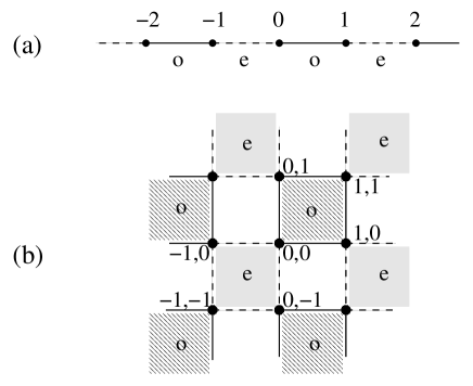
Figure 1: Bipartite decomposition of the hypercubic lattice in to odd and even parts: (a) for $d=1$, (b) for $d=2$.

Even when the Hamiltonian $H$ is local, the discrete time evolution operator $U=\exp(-iH\tau)$ may connect arbitrarily separated vertices. To make $U$ also local, we split $H$ in to block-diagonal Hermitian parts and then exponentiate each part separately qwalk1 . For a bipartite lattice, partitioning of $H$ in to two parts (which we label “odd” and “even”) is sufficient for this purpose spinorsize :

$$H_{\rm free}=H_{o}+H_{e}~{}.$$ (6)

This partition is illustrated in Fig.1 for $d=1$ and $d=2$. Each part contains all the vertices, but only half of the links attached to each vertex. Each link is associated with a term in $H_{\rm free}$ providing propagation along it, and appears in only one of the two parts. $H$ thus gets divided in to a set of non-overlapping blocks of size $2^{d}\times 2^{d}$ (each block corresponds to an elementary hypercube on the lattice) that can be exactly exponentiated. The amplitude distribution then evolves according to

$$\psi(\vec{x};t)=W^{t}\psi(\vec{x};0)~{},~{}~{}W=U_{e}U_{o}=e^{-iH_{e}\tau}e^{-iH_{o}\tau}~{}.$$ (7)

Each block of the unitary matrices $U_{o(e)}$ mixes amplitudes of vertices belonging to a single elementary hypercube, and the amplitude distribution spreads in time because the two alternating matrices do not commute. Note that $W$ does not perform evolution according to $H_{\rm free}$ exactly. Instead, $W=\exp(-iH_{\rm free}\tau)+O(\tau^{2})$. Still, the truncation is such that $W$ is exactly unitary, i.e. $W=\exp(-i\tilde{H}\tau)$ for some $\tilde{H}$.

We adopt the convention where the walk operator $W$ is real. For $d=1$, we set

$$H_{o}|x\rangle = -{i\over 2}\Big{[}(-1)^{x}|x+(-1)^{x}\rangle\Big{]}~{},$$ (8)

$$H_{e}|x\rangle = {i\over 2}\Big{[}(-1)^{x}|x-(-1)^{x}\rangle\Big{]}~{}.$$ (9)

The resultant Hamiltonian blocks are $H_{o}^{B}=-\sigma_{2}/2$, and $H_{e}^{B}=\sigma_{2}/2$ when operating on the block with coordinates flipped in sign. With $(H_{o}^{B})^{2}=(H_{e}^{B})^{2}={1\over 4}I$,

$$U_{o(e)}=cI-2isH_{o(e)}~{},~{}~{}|c|^{2}+|s|^{2}=1~{},$$ (10)

where $s=\sin(\tau/2)$ is a parameter that can be tuned.

These expressions can be rearranged to separate the translationally invariant part of the walk from the location dependent signs. Let the amplitude distribution in a two spinor (or coin) component notation be

$$\Psi(X,t)\equiv\left(\matrix{\psi(2x,t)\cr\psi(2x-1,t)\cr}\right)~{}.$$ (11)

Then the walk operator becomes

$$W = \tilde{U}C~{},~{}~{}C=U_{o}^{B}=\left(\matrix{c&s\cr-s&c\cr}\right)~{},$$ (12)

$$\tilde{U}|X\rangle = c|X\rangle-s\sum_{\pm}(\pm\sigma_{\pm})|X\pm 1\rangle~{}.$$ (13)

The operator $C=U_{o}^{B}$ just mixes the components of $\Psi$ within the block. The first term of the operator $\tilde{U}$ is stationary, while the other moves the amplitude to neighbouring blocks. The movement is accompanied by chirality flip, a characteristic feature of the Dirac operator, because of the raising and lowering Pauli operators $\sigma_{\pm}=(\sigma_{1}\pm i\sigma_{2})/2$.

In $d$ dimensions, the preceding structure generalises to $2^{d}\times 2^{d}$ Hamiltonian blocks that can be expressed in terms of tensor products of Pauli matrices qwalk2 . When operating on hypercubes with coordinate labels $\{0,1\}^{\otimes d}$,

$$H_{o}^{B}=-{1\over 2}\sum_{j=1}^{d}I^{\otimes(d-j)}\otimes\sigma_{2}\otimes\sigma_{3}^{\otimes(j-1)}~{},$$ (14)

and $H_{e}^{B}=-H_{o}^{B}$ when operating on a hypercube with all coordinates flipped in sign. Note that Eq.(14) is the sum of $d$ terms, which mutually anticommute and whose squares are proportional to identity. This is the characteristic signature of the Dirac Hamiltonian, Eq.(1). The block-diagonal matrices satisfy $H_{o}^{2}=H_{e}^{2}={d\over 4}I$, and exponentiate to

$$U_{o(e)}=cI-is{2\over\sqrt{d}}H_{o(e)}~{},~{}~{}|c|^{2}+|s|^{2}=1~{}.$$ (15)

The parameter $s=\sin(\sqrt{d}\tau/2)$ can be optimised, to achieve the fastest diffusion across the lattice. Note that the $d$-dimensional walk is not the tensor production of $d$ one-dimensional walks.

Again separating the degrees of freedom within each local hypercube as $\vec{x}\equiv\vec{X}\otimes${0,-1}^⊗d, the location dependent signs can be rewritten as operators acting on the spinor (or coin) degrees of freedom. The walk operator takes the form: $W=\tilde{U}C$, $C=U_{o}^{B}$, and

$$\tilde{U}|\vec{X}\rangle = c|\vec{X}\rangle$$

$$- \frac{s}{\sqrt{d}}\sum_{\pm}\sum_{j=1}^{d}(I^{\otimes(j-1)}\otimes(\pm\sigma_{\pm})\otimes\sigma_{3}^{\otimes(d-j)})|\vec{X}\pm\hat{j}\rangle~{}.$$

I.2 Search Algorithm

To search for a marked vertex, say the origin, we attract the quantum random walk toward it by adding a potential to the free Hamiltonian,

$$V=\cases{\beta V_{0}~{}\delta_{\vec{x},0}~{}~{}({\rm gravitational})~{},\cr V_{0}~{}\delta_{\vec{x},0}~{}~{}({\rm electromagnetic})~{}.}$$ (17)

Exponentiation of this potential produces a phase change for the amplitude at the marked vertex. For the steepest attraction of the quantum random walk toward the marked vertex, it is optimal to choose $V_{0}$ so as to make the corresponding evolution phase maximally different from $1$, i.e. $e^{-iV_{0}\tau}=-1$. The sign provided by $\beta$ does not matter in this case, and the evolution phase becomes the binary oracle,

$$R=I-2|\vec{0}\rangle\langle\vec{0}|~{}.$$ (18)

The search algorithm alternates between diffusion and oracle operators—a discrete version of Trotter’s formula involving $H_{o}$, $H_{e}$ and $V$—yielding the evolution

$$\psi(\vec{x};t_{1},t_{2})=[W^{t_{1}}R]^{t_{2}}\psi(\vec{x};0,0)~{}.$$ (19)

Here $t_{2}$ is the number of search oracle queries, and $t_{1}$ is the number of walk steps between queries. Both should be minimised to find the the quickest solution to the search problem.

Since this algorithm iterates a unitary operator on the initial state, it produces periodic results. As a function of the number of iterations, the probability of being at the marked vertex first increases, reaches a peak value $P$ after $t_{2}$ search oracle queries, then decreases toward zero, and thereafter keeps on repeating this cycle. Grover’s algorithm is designed to evolve the quantum state in a two-dimensional Hilbert space (spanned by the initial and marked states), and is able to reach $P=1$. That does not hold for spatial search, and the resultant values of $P$ are less than $1$. The remedy is to augment the algorithm by the amplitude amplification procedure BHMT , to find the marked vertex with $\Theta(1)$ probability. The complexity of the algorithm is then characterised by the effective number of search oracle queries, $t_{2}/\sqrt{P}$.

I.3 Complexity Bounds

Spatial search obeys two simple lower bounds. One arises from the fact that while the marked vertex could be anywhere on the lattice, one step of the local walk can move from any vertex to only its nearest neighbours. Since the marked vertex cannot be located without reaching it, the worst case scenario on a hypercubic lattice requires $\Omega(dL)$ steps. This bound is the strongest in one dimension, where quantum search is unable to improve on the $O(N)$ classical search.

The other bound follows from the fact that spatial search cannot outperform Grover’s optimal algorithm, and so it must require $\Omega(\sqrt{N})$ oracle queries. That is independent of $d$, and stronger than the first bound for $d>2$. As a matter of fact, the first bound weakens with increasing $d$, as the number of neighbours of a vertex increase and steps required to go from one corner of the lattice to another decrease. In analogy with mean field theory behaviour of problems in statistical mechanics, we can thus expect that in the $d\rightarrow\infty$ limit the locality restriction on the walk would become irrelevant and the complexity of spatial search would approach that of Grover’s algorithm. (Note that the maximum value of $d$ is $\log_{2}N$ for finite $N$.) Our results in this work demonstrate that not only is the $\Omega(\sqrt{N})$ complexity scaling achievable for $d>2$, but one can get pretty close to the asymptotic prefactor $\pi/4$ as well.

Combined together, the two bounds make the complexity of spatial search $\Omega(dN^{1/d},\sqrt{N})$. The two bounds are of the same magnitude, $\Omega(\sqrt{N})$, for the critical case of $d=2$. It is a familiar occurrence in statistical mechanics of critical phenomena that an interplay of different dynamical features produces logarithmic correction factors in critical dimensions due to infrared divergences. The same seems to be true for spatial search in $d=2$, where algorithms are slowed down by extra logarithmic factors gridsrch1 ; gridsrch2 ; tulsi . It is an open question to design algorithms, perhaps using additional parameters, that suppress the logarithmic factors as much as possible. We look at the special $d=2$ case in an accompanying article.

The way the lower bounds arise in spatial search also illustrates an interplay of two distinct physical principles, special relativity (or no faster than light signaling) and unitarity. It is well-known that the two are compatible, but just barely so, in the sense that physical theories that are unitary but not relativistic or relativistic but not unitary exist. Furthermore, the best algorithms should arise in a framework that respects both the principles, i.e. relativistic quantum mechanics. In spatial search, locality of the quantum walk and the square-root speed up produced by the Dirac equation (through change in the dispersion relation) follow from special relativity. On the other hand, optimality of square-root speed up provided by Grover’s algorithm is a consequence of unitarity BBBV ; zalka . Why these two distinct physical principles lead to the same scaling constraint is not understood, and is a really interesting question to explore. At present, however, we have nothing more to add.

We point out that preparation of the unbiased initial state for the search problem, i.e. the translationally invariant uniform superposition state $|s\rangle=\sum_{x}|\vec{x}\rangle/\sqrt{N}$, is not at all difficult using local directed walk steps. For instance, one can start at the origin, step by step transfer the amplitude to the next vertex along an axis, and achieve an amplitude $L^{-1/2}$ at all the vertices on the axis after $L$ steps. Repeating the procedure for each remaining coordinate direction produces the state $|s\rangle$ after $dL$ steps in total. Clearly, this preparation does not add to the complexity of the algorithm.

II Optimisation of Parameters

The fastest search amounts to finding the shortest unitary evolution path between the initial state $|s\rangle$ and the marked state $|\vec{0}\rangle$. This path is a geodesic arc on the unitary sphere from $|s\rangle$ to $|\vec{0}\rangle$, and Grover’s optimal algorithm strides along this path perfectly. In our algorithm, Eq.(19), we have replaced Grover’s optimal diffusion operator, $G=2|s\rangle\langle s|-1$, with the walk operator $W^{t_{1}}$. So to optimise our algorithm, we need to tune the parameters appearing in $W^{t_{1}}$, i.e. $s$ (or $c$) and $t_{1}$, such that $W^{t_{1}}R$ approximates a rotation in the two-dimensional $|s\rangle$-$|\vec{0}\rangle$ subspace by the largest possible angle.

The operator $G$ has $|s\rangle$ as an eigenstate with eigenvalue $1$. All other states orthogonal to $|s\rangle$, in particular the combination $|s_{\perp}\rangle=(|s\rangle-\sqrt{N}|\vec{0}\rangle)/\sqrt{N-1}$ in the $|s\rangle$-$|\vec{0}\rangle$ subspace, are its eigenstates with eigenvalue $-1$. The walk operator $W=U_{e}U_{o}$ also has $|s\rangle$ as an eigenstate with eigenvalue $1$. However, its other eigenvalues are spread around the unit circle, and evolution under $W^{t_{1}}R$ does not remain fully confined to the $|s\rangle$-$|\vec{0}\rangle$ subspace. If the outward diffusion is not controlled, the probability of remaining in the $|s\rangle$-$|\vec{0}\rangle$ subspace would decay exponentially with the number of iterations. To reach the marked state with a constant probability, therefore, parameters must be tuned so that part of the outward diffusion subsequently returns to the $|s\rangle$-$|\vec{0}\rangle$ subspace.

II.1 Analytical Criteria

The optimisation condition that makes $W^{t_{1}}$ as close an approximation to $G$ as possible can be formulated in several different ways. Though they all lead to the same result, describing them separately is instructive.

(1) Maximise the overlap of $W^{t_{1}}$ and $G$, i.e.

$$Tr(W^{t_{1}}G)=Tr(2|s\rangle\langle s|-W^{t_{1}})=2-\sum_{i}\langle i|W^{t_{1}}|i\rangle~{}.$$ (20)

$\langle i|W^{t_{1}}|i\rangle$ is the amplitude for the random walk to return to the starting state $|i\rangle$ after $t_{1}$ time steps. Since $W$ is translationally invariant along each coordinate direction in steps of 2, we need to evaluate $\langle i|W^{t_{1}}|i\rangle$ only for states $|i\rangle$ in an elementary hypercube. Now, any closed path on a hypercubic lattice takes an even number of steps along each coordinate direction, and all location dependent propagation signs (cf. Eq.(4)) get squared to $1$ in the process. As a result, $\langle i|W^{t_{1}}|i\rangle$ is independent of $|i\rangle$, and the optimisation condition becomes the minimisation of $A(t_{1})\equiv\langle\vec{0}|W^{t_{1}}|\vec{0}\rangle$.

(2) Make $|s_{\perp}\rangle$ approximate an eigenvector of $W^{t_{1}}$, with an eigenvalue approaching $-1$, i.e. minimise

$$\langle s_{\perp}|W^{t_{1}}|s_{\perp}\rangle={1\over N-1}\big{(}-1+NA(t_{1})\big{)}~{},$$ (21)

which happens to be the same condition as given earlier. In addition, unitarity of the evolution operator implies

$$|\langle s_{\perp}|W^{t_{1}}|s_{\perp}\rangle|\leq 1~{}\Longrightarrow~{}-1+{\textstyle 2\over N}\leq A(t_{1})\leq 1~{}.$$ (22)

(3) Maximise the rotation provided by the operator $W^{t_{1}}R$ along the $|s\rangle$-$|\vec{0}\rangle$ subspace. This rotation is given by the projection

$${\rm Proj}_{s,s_{\perp}}[W^{t_{1}}R]=\pmatrix{\langle s|W^{t_{1}}R|s\rangle&\langle s|W^{t_{1}}R|s_{\perp}\rangle\cr\langle s_{\perp}|W^{t_{1}}R|s\rangle&\langle s_{\perp}|W^{t_{1}}R|s_{\perp}\rangle\cr}$$

$$=\pmatrix{1-{2\over N}&{2\over N}\sqrt{N-1}\cr{2\over\sqrt{N-1}}(A(t_{1})-{1\over N})&(1-{2\over N}){1-NA(t_{1})\over N-1}\cr}$$ (23)

$$=\pmatrix{1&0\cr 0&{1-NA(t_{1})\over N-1}\cr}\pmatrix{1-{2\over N}&{2\over N}\sqrt{N-1}\cr-{2\over N}\sqrt{N-1}&1-{2\over N}\cr}~{}.$$

The factor on the right in Eq.(23) is precisely the rotation matrix produced by the operator $GR$ in Grover’s algorithm, i.e. rotation by an angle $2\sin^{-1}(1/\sqrt{N})$ in the $|s\rangle$-$|\vec{0}\rangle$ subspace. So the total projection can be viewed as first applying an iteration of Grover’s algorithm to the state, and then shrinking the $|s_{\perp}\rangle$ component by a factor $(1-NA(t_{1}))/(N-1)$. The shrinking disappears and the projection tends to an exact orthogonal transformation, as $A(t_{1})$ approaches its lower bound $(2-N)/N$. It also follows that when the shrinking is controlled, cutting down outward diffusion from the $|s\rangle$-$|\vec{0}\rangle$ subspace, the algorithm will have the same $O(\sqrt{N})$ scaling as in case of Grover’s algorithm.

The minimisation condition for $A(t_{1})$ is obtained here only using the translational invariance of the walk operator $W$, together with $W|s\rangle=|s\rangle$ and $\langle s|W=\langle s|$. It is easy to perform this optimisation numerically, as a function of the parameters $s$ and $t_{1}$, and our results are described later. Before that, an understanding of the eigenspectrum of $W$ gives us some idea regarding what to expect.

Since $H_{o}^{2}=H_{e}^{2}=\frac{d}{4}I$, eigenvalues of $H_{o}$ and $H_{e}$ are $\pm\sqrt{d}/2$. Moreover, $H_{o}$ and $H_{e}$ are traceless, so that half the eigenvalues are $\sqrt{d}/2$ and the other half $-\sqrt{d}/2$. Consequently, eigenvalues of $U_{o}$ and $U_{e}$ are $c\pm is=\exp(\pm i\sqrt{d}\tau/2)$, equally divided among complex conjugate pairs. Furthermore, $H_{o(e)}$ and $U_{o(e)}$ have the same eigenvectors.

Since $U_{o}$ and $U_{e}$ do not commute, we do not have a general solution for the eigenspectrum of $W$. Still it is straightforward to work it out in the continuum time limit, $\tau\rightarrow 0$. $H_{\rm free}$ is diagonalised by a Fourier transform,

$$H_{\rm free}^{2}|\vec{x}\rangle = -\frac{1}{4}\sum_{n=1}^{d}\Big{[}|\vec{x}+2\hat{n}\rangle-2|\vec{x}\rangle+|\vec{x}-2\hat{n}\rangle\Big{]}$$ (24)

$$\longrightarrow \sum_{n=1}^{d}\sin^{2}(k_{n})|\vec{k}\rangle~{},$$

with a uniform distribution in the Brillouin zone. Up to $O(\tau^{2})$, therefore, the eigenvalues of $W(\approx e^{-iH_{\rm free}\tau})$ are $\exp(\pm i\tau\sqrt{\sum_{j}\sin^{2}k_{j}})$, with the eigenphases in the interval $[-\tau\sqrt{d},\tau\sqrt{d}]$. The average value of $H_{\rm free}^{2}$ is $d/2$, and the corresponding eigenvalues of $W$ are $\exp(\pm i\tau\sqrt{d/2})$. We find that this average value plays an important role in determination of the optimal parameters.

II.2 Numerical Optimisation

The considerations of the previous subsection focused on what happens during a single iteration of the algorithm. Over many iterations, there is outward diffusion of the amplitude distribution from the $|s\rangle$-$|\vec{0}\rangle$ subspace, and subsequent partial return. That plays an important role in the overall success of the algorithm, but we have not been able to estimate it analytically. To study the performance of the whole algorithm, therefore, we numerically tune the parameters $s$ and $t_{1}$ to (a) maximise the probability of reaching the marked vertex, and (b) minimise the number of search oracle queries required to reach that stage. The ensuing results of our optimisation of $P$, $t_{2}$ and $A(t_{1})$ are described in what follows.

We first looked at how the probability distribution evolves as a function of time during the search process. To illustrate our results, we take $s=c=1/\sqrt{2}$ that corresponds to maximal mixing between even and odd vertices, and analyse the evolution as a function of $t_{1}$ and $t_{2}$ on a $32^{3}$ lattice. As displayed in Fig.2, the probability at the marked vertex undergoes a cyclic evolution pattern as a function of time $t_{2}$. We observe that the evolution is essentially sinusoidal for $t_{1}=1,2,3$, and persists for more than 30 cycles without any visible deviation. This behaviour implies that a constant fraction of the quantum state remains in the $|s\rangle$-$|\vec{0}\rangle$ subspace, and the operator $W^{t_{1}}R$ rotates it at a uniform rate within the subspace, fully matching the exact solution of Grover’s algorithm. The difference among $t_{1}=1,2,3$ is that the cycle time and the peak probability vary, meaning that the fraction of the quantum state present in the $|s\rangle$-$|\vec{0}\rangle$ subspace depends on $t_{1}$.

For $t_{1}>3$, we find that the evolution rapidly loses its sinusoidal nature and the peak probability plummets. The change in the pattern is so drastic that the algorithm no longer performs a reasonable search. This behaviour implies that most of the quantum state has moved out of the $|s\rangle$-$|\vec{0}\rangle$ subspace and only a negligible component is left behind. An appropriate choice of $t_{1}$ is thus crucial for constructing a successful search algorithm.

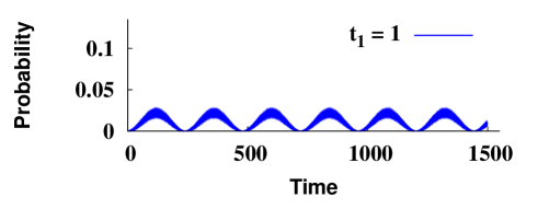
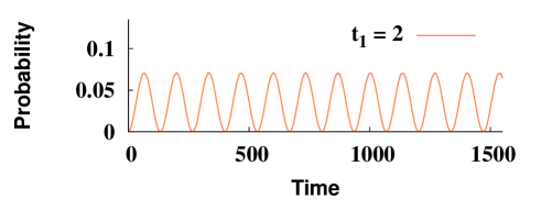
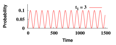
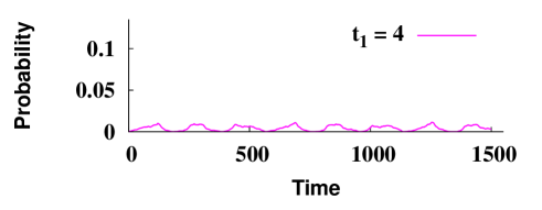
Figure 2: (Color online) Time evolution of the probability at the marked vertex for the spatial search problem on a $32^{3}$ lattice. $s=1/\sqrt{2}$ and $t_{1}$ increases from $1$ (top) to $4$ (bottom).

We also show in Fig.3 what the probability distribution looks like at the instance when the probability at the marked vertex attains its peak value. We note that the distribution is strongly peaked around the marked vertex in an essentially uniform background. The peak is sharper when the peak probability is larger, and it almost disappears for $t_{1}>3$. This pattern suggests that the part of the quantum state that diffuses outside the $|s\rangle$-$|\vec{0}\rangle$ subspace is almost featureless.

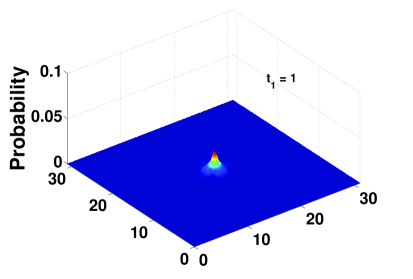
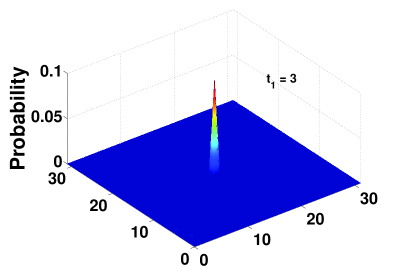
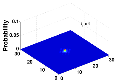
Figure 3: (Color online) Probability distribution for the spatial search problem on a $32^{3}$ lattice, at the instance when the probability at the marked vertex $(16,16,16)$ attains its peak value. The displayed results are for the $z=16$ slice. $s=1/\sqrt{2}$ and $t_{1}$ increases from $1$ (top) to $4$ (bottom).

Combining our observations in this particular example, we find that the best results—the shortest period, the largest peak probability and the sharpest peak—clearly correspond to $t_{1}=3$. The results improve as $t_{1}$ increases from $1$ to $3$, and rapidly deteriorate thereafter. The important fact that all optimal features appear simultaneously at $t_{1}=3$ simplifies tuning of the parameters.

Next we scanned through values of $s$, for different values of $t_{1}$ and in different dimensions, to determine the optimal values at which the peak probability $P$ at the marked vertex is the largest and the time $t_{2}$ required to reach it is the smallest. A typical situation, with $t_{1}=3$ on a $32^{3}$ lattice, is shown in Fig.4. We notice that continuous $P$ has a smoother behaviour than discrete $t_{2}$, and maximisation of $P$ and minimisation of $t_{2}$ occur at roughly the same value of $s$. So we simplify matters, and select maximisation of $P$ as our optimality condition.

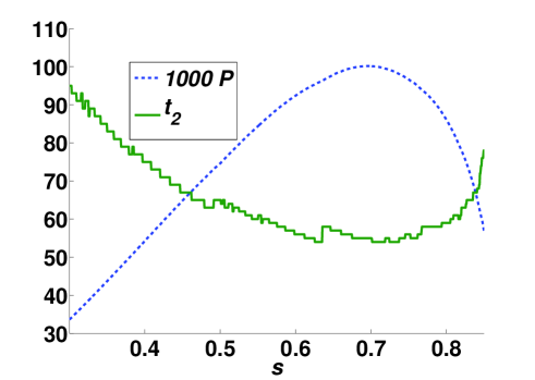
Figure 4: (Color online) Optimisation of $s$ for $t_{1}=3$ on a $32^{3}$ lattice, using peak probability $P$ as well as oracle queries $t_{2}$.

A comparison of our scans, for $t_{1}=3$ and different number of dimensions, is presented in Fig.5. We find that at fixed $t_{1}$, the shape of the $P$ vs. $s$ curve is almost dimension independent, and the optimal value of $s$ is approximately the same for all dimensions. We also observe that for fixed $s$, $P$ roughly scales as $2^{-d}$. In the staggered fermion implementation of the Dirac operator, different vertices of an elementary hypercube correspond to different degrees of freedom staggered . So our observation suggests that to a large extent only the degree of freedom corresponding to the marked vertex evolves during the search, while other degrees of freedom remain spectators. Moreover, the feature that the maximum value of $P$ approaches $2^{-d}$ with increasing $d$ implies that the efficiency of our algorithm increases with $d$.

Table 1: Results of optimal parameter determination for different $t_{1}$ and in different dimensions.

$d$	$L$	$t_{1}$	Spatial Search				Walk
			$s$	$t_{2}$	$P$	$\theta$	$s$	$A(t_{1})_{\rm min}$	$\theta$
3	32	2	0.9507	59	0.0942	3.551	0.9258	$-$0.7143	3.346
		3	0.7015	55	0.1001	3.299	0.6737	$-$0.7618	3.136
		4	0.5363	55	0.1016	3.202	0.5194	$-$0.7748	3.089
		8	0.2755	54	0.1027	3.158	0.2665	$-$0.7860	3.052
		20	0.1114	54	0.1030	3.157	0.1074	$-$0.7890	3.044
4	16	2	0.9541	54	0.0528	3.583	0.9428	$-$0.7778	3.482
		3	0.6986	54	0.0548	3.281	0.6827	$-$0.8190	3.188
		4	0.5411	53	0.0553	3.234	0.5257	$-$0.8300	3.131
		8	0.2771	52	0.0558	3.177	0.2694	$-$0.8395	3.086
		20	0.1115	52	0.0559	3.160	0.1084	$-$0.8420	3.072
5	16	2	0.9500	150	0.0276	3.545	0.9535	$-$0.8182	3.577
		3	0.6920	148	0.0284	3.242	0.6880	$-$0.8541	3.219
		4	0.5376	147	0.0286	3.211	0.5292	$-$0.8636	3.155
		8	0.2726	147	0.0288	3.124	0.2710	$-$0.8718	3.105
		20	0.1108	147	0.0288	3.140	0.1092	$-$0.8739	3.095
6	8	3	0.6891	51	0.0145	3.225	0.6913	$-$0.8778	3.238
		20	0.1106	51	0.0147	3.135	0.1094	$-$0.8951	3.101
7	8	3	0.6932	102	0.0073	3.250	0.6937	$-$0.8949	3.252
		20	0.1097	102	0.0074	3.109	0.1098	$-$0.9102	3.112

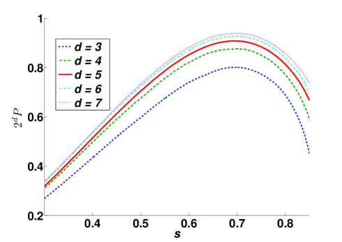
Figure 5: (Color online) Optimisation of $s$ for $t_{1}=3$ in different dimensions. Lattice sizes $L=32,16,16,8,8$ were used for $d=3,4,5,6,7$, respectively.

All our quantitative results for optimal values of $s$ are collected in Table I. We note that the best performance parameters, $P$ and $t_{2}$, depend on $d$ but hardly on $t_{1}$ or $s$. (With increasing $t_{1}$, there is a slight increase in $P$ and a small decrease in $t_{2}$, but that is a rather tiny improvement.) More interestingly, we find a relation between the optimal values of $s$ and $t_{1}$, in terms of the variable

$$\theta=\sqrt{2}t_{1}\sin^{-1}s=t_{1}\tau\sqrt{d/2}~{}.$$ (25)

Since $\sin^{-1}s$ describes the unitary rotation performed by the single step operators $U_{o(e)}$, and $t_{1}$ is the number of walk steps, $\theta$ is a measure of the unitary rotation performed by the operator $W^{t_{1}}$. The corresponding operator in Grover’s optimal algorithm, $G$, is a reflection providing a phase change of $\pi$. We find that our optimal $W^{t_{1}}$ is also close to a reflection, in a sense, with $\theta\approx\pi$. Unlike the discrete $\pm 1$ eigenvalues of $G$ though, eigenvalues of $W^{t_{1}}$ form a distribution. We do not know this distribution in general, but we know it in the limit $\tau\rightarrow 0$, as described at the end of Subsection II.A. This limit corresponds to small $s$ and large $t_{1}$, and Table I shows that $\theta$ indeed gets close to $\pi$ in this limit. To be precise, this normalisation of $\theta$ implies that the optimal $W^{t_{1}}\equiv e^{-i\tilde{H}\tau t_{1}}$ is a reflection operator for the “average eigenvalue” of the associated $\tilde{H}^{2}$. Appearance of the average eigenvalue in the normalisation indicates that all spatial modes contribute to the search process with roughly equal strength.

Table I also lists our results for the variable $A(t_{1})$ defined in Subsection II.A, which characterises how close $W^{t_{1}}$ is to $G$. We computed $A(t_{1})$, by starting with unit amplitude at the marked vertex, and then measuring the amplitude at the marked vertex after $t_{1}$ walk steps. At the beginning of this subsection we mentioned that checking $A(t_{1})$ is not as elaborate an optimisation test as using the full search algorithm. Nevertheless, the results corroborate our optimisation of spatial search: The minimum value of $A(t_{1})$ is reasonably close to $-1$, and occurs at approximately the same value of $s$ (and hence $\theta$) that provides the optimal search (the mismatch decreases with increasing $d$). We also observe that $A(t_{1})$ gets closer to $-1$, suggesting that the algorithm becomes more efficient, with increasing $d$ as well as $t_{1}$.

Given the strong correlation between the optimal values of $s$ and $t_{1}$, the computational cost of the algorithm is minimised by choosing the smallest $t_{1}$. For $t_{1}=1$, Eq.(25) does not have a solution with $\theta\approx\pi$, the optimal value of $s$ is very close to $1$, and our algorithm does not work well there. Then $t_{1}=2$ is the choice that minimises the number of walk steps in the algorithm. Even when the emphasis is on optimising $P$ and $t_{2}$, most of the improvement can be obtained by going from $t_{1}=2$ to $t_{1}=3$, and we need not go beyond that.

III Simulation Results

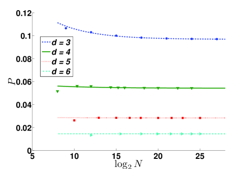
Figure 6: (Color online) Peak probability at the marked vertex as a function of database size (ranging from $2^{8}$ to $2^{27}$) in different dimensions. The points are the data from the simulations with $t_{1}=3$, and the curves are the fits $P=a_{1}+(b_{1}/L)$.

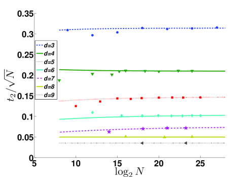
Figure 7: (Color online) Number of search oracle queries as a function of database size (ranging from $2^{8}$ to $2^{27}$) in different dimensions. The points are the data from the simulations with $t_{1}=3$, and the curves are the fits $(t_{2}/\sqrt{N})=a_{2}+(b_{2}/L)$.

We carried out numerical simulations of the quantum spatial search problem, with a single marked vertex and lattice dimension ranging from $3$ to $9$. The matrices $U_{o(e)}$ are real with our conventions, and that was convenient for simulations. The optimal values of $s$-$t_{1}$ pairs depend a little on the lattice size and dimension. We are only interested in the asymptotic behaviour of the algorithm, however, so we used the same parameter values for all lattice sizes and dimensions: $s=0.9539$ for $t_{1}=2$, $s=1/\sqrt{2}$ for $t_{1}=3$ and $s=0.5410$ for $t_{1}=4$.

To extract the scaling properties of the algorithm, we studied the behaviour of $P$ and $t_{2}$, as a function of $L$ and $d$. We found that the finite size effects in our data, as $L\rightarrow\infty$ at fixed $d$, are well described by series in inverse powers of $L$. In Figs.6-7, we show some of our results with the fitting functions:

$$P=a_{1}+{b_{1}\over L}~{},~{}~{}{t_{2}\over\sqrt{N}}=a_{2}+{b_{2}\over L}~{}.$$ (26)

All the fit parameters are listed in Table II, where error refers to the r.m.s. deviation of the data from the fit. We do not have sufficient data for $d=8$ and $d=9$, to make accurate fits or to see the asymptotic behaviour. Our analysis, therefore, relies on the patterns seen for $d=3$ to $d=7$, while we use $d=8$ and $d=9$ values only for consistency checks.

Table 2: Fit parameters for peak probability $P$ and search oracle queries $t_{2}/\sqrt{N}$ vs. $L$.

$s$	$t_{1}$	$d$	$L$	$a_{1}$	$b_{1}$	Error	$a_{2}$	$b_{2}$	Error	$a_{2}/\sqrt{a_{1}}$
0.9539	2	3	64,128,256,512	0.0911	$-$0.0964	2.43$\times$$10^{-5}$	0.3237	$-$0.1440	4.57$\times$$10^{-4}$	1.072
		4	16,32,48,64	0.0522	$-$0.0100	3.02$\times$$10^{-5}$	0.2167	$-$0.0832	1.05$\times$$10^{-3}$	0.948
		5	12,16,24,32	0.0275	$-$0.0009	1.70$\times$$10^{-6}$	0.1486	$-$0.0243	2.39$\times$$10^{-4}$	0.896
		6	12,14,16,18	0.0141	$-$0.0001	2.31$\times$$10^{-7}$	0.1043	$-$0.0208	1.78$\times$$10^{-4}$	0.878
		7	6,8,10	0.0072	$-$0.0004	1.40$\times$$10^{-6}$	0.0757	$-$0.0338	2.47$\times$$10^{-4}$	0.892
		8	6,8	0.0036	—	3.50$\times$$10^{-6}$	0.0509	—	7.23$\times$$10^{-5}$	0.848
		9	6	0.0018	—	—	0.0356	—	—	0.839
1/$\sqrt{2}$	3	3	64,128,256,512	0.0968	$-$0.0920	2.73$\times$$10^{-6}$	0.3141	$-0.0306$	1.23$\times$$10^{-3}$	1.010
		4	16,32,48,64	0.0542	$-$0.0076	1.46$\times$$10^{-5}$	0.2097	$-$0.0151	6.71$\times$$10^{-4}$	0.901
		5	12,16,24,32	0.0283	$-$0.0010	4.66$\times$$10^{-6}$	0.1470	$-$0.0300	2.12$\times$$10^{-4}$	0.874
		6	12,14,16,18	0.0145	$-$0.0001	5.79$\times$$10^{-7}$	0.1035	$-$0.0269	1.88$\times$$10^{-4}$	0.860
		7	6,8,10	0.0074	$-$0.0003	1.46$\times$$10^{-6}$	0.0750	$-$0.0296	3.39$\times$$10^{-4}$	0.872
		8	6,8	0.0037	—	3.00$\times$$10^{-6}$	0.0498	—	4.55$\times$$10^{-5}$	0.819
		9	6	0.0019	—	—	0.0353	—	—	0.810
0.5410	4	3	64,128,256,512	0.0984	$-$0.0936	1.84$\times$$10^{-5}$	0.3123	$-$0.1239	8.46$\times$$10^{-4}$	0.996
		4	16,32,48,64	0.0548	$-$0.0087	2.24$\times$$10^{-5}$	0.2103	$-$0.0500	3.57$\times$$10^{-4}$	0.898
		5	12,16,24,32	0.0285	$-$0.0013	8.05$\times$$10^{-6}$	0.1455	$-$0.0142	2.25$\times$$10^{-4}$	0.862
		6	12,14,16,18	0.0146	$-$0.0002	7.67$\times$$10^{-7}$	0.1015	$-$0.0043	6.28$\times$$10^{-5}$	0.840
		7	6,8,10	0.0074	$-$0.0003	2.86$\times$$10^{-6}$	0.0733	$-$0.0194	2.01$\times$$10^{-4}$	0.852
		8	6,8	0.0037	—	4.50$\times$$10^{-6}$	0.0505	—	4.39$\times$$10^{-4}$	0.830
		9	6	0.0019	—	—	0.0353	—	—	0.810

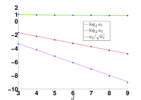
Figure 8: (Color online) Behaviour of the asymptotic fit parameters as a function of dimension. The data points are from Table II, with $t_{1}=3$, and the curves are the fits described in Eqs.(27,28).

We observe the following features:
(1) There is not much difference among the $a_{1}$ and $a_{2}$ values for different optimised $s$-$t_{1}$ pairs. This confirms our earlier inference that implementing our algorithm for $t_{1}=2$ minimises the running cost.
(2) $P$ approaches a constant as $L\rightarrow\infty$, with $a_{1}$ decreasing approximately as $2^{-d}$ with increasing $d$. As mentioned before, this is a consequence of the fact that in the staggered fermion implementation of the Dirac operator, only the degree of freedom corresponding to the location of the marked vertex on the elementary hypercube participates in the search process. Since the number of vertices in an elementary hypercube is $2^{d}$, $P$ is upper bounded by $2^{-d}$. Our algorithm achieves that bound up to a constant multiple close to $1$.
(3) $b_{1}$ decreases toward zero with increasing $d$, which is also true for $|b_{2}|$ to a large extent. Thus the smallest $d=3$ has the largest finite size corrections to the asymptotic $L\rightarrow\infty$ behaviour. This suggests that as the number of neighbours of a vertex increase, the finite size of the lattice becomes less and less relevant.
(4) $t_{2}$ is proportional to $\sqrt{N}$ as $L\rightarrow\infty$, with $a_{2}$ decreasing approximately as $2^{-d/2}$ with increasing $d$. Thus $t_{2}$ scales with the database size as $(L/2)^{d/2}=\sqrt{N/2^{d}}$. This is in agreement with the fact that, with only one degree of freedom per elementary hypercube participating in the search process, the effective number of vertices being searched is $N/2^{d}$.
(5) In the combination $t_{2}/\sqrt{P}$, describing the effective number of oracle queries for our algorithm, the factors of $2^{d}$ arising from the number of vertices in an elementary hypercube fully cancel. That makes $t_{2}/\sqrt{P}$ scale as $\sqrt{N}$, and $a_{2}/\sqrt{a_{1}}$ describes the complexity scaling of our algorithm. As listed in the rightmost column of Table II, $a_{2}/\sqrt{a_{1}}$ shows a gradual decrease with increasing $d$, and our results are just above the corresponding value $\pi/4$ for Grover’s optimal algorithm. More explicitly, our result for $d=3$ is about 25% above $\pi/4$, decreasing to about 10% above $\pi/4$ for $d=7$. These values imply that our algorithm improves in efficiency with increasing $d$, and is not too far from the optimal behaviour even for the smallest dimension $d=3$.

To analyse the dimension dependence of our algorithm in more detail, we fit the values in Table II to the functional forms,

$$\log_{2}a_{1}=c_{1}+d_{1}d~{},~{}~{}\log_{2}a_{2}=c_{2}+d_{2}d~{},~{}~{}$$ (27)

$${a_{2}\over\sqrt{a_{1}}}=c_{3}+{d_{3}\over d}~{}.$$ (28)

The results for $t_{1}=3$ are displayed in Fig.8, showing that the fits work reasonably well.

Table 3: Fit parameters for $\log_{2}a_{1}$, $\log_{2}a_{2}$ and $a_{2}/\sqrt{a_{1}}$ vs. $d$.

$s$	$t_{1}$	Fitted $d$	$c_{1}$	$d_{1}$	Error	$c_{2}$	$d_{2}$	Error	$c_{3}$	$d_{3}$	Error
0.9539	2	3,4,5,6,7,8	$-$0.553	$-$0.938	4.77$\times 10^{-2}$	$-$0.085	$-$0.526	2.53$\times 10^{-2}$	0.721	0.995	1.71$\times 10^{-2}$
$1/\sqrt{2}$	3		$-$0.458	$-$0.947	4.48$\times 10^{-2}$	$-$0.138	$-$0.521	2.57$\times 10^{-2}$	0.729	0.791	1.63$\times 10^{-2}$
0.5410	4		$-$0.421	$-$0.951	3.78$\times 10^{-2}$	$-$0.151	$-$0.521	2.09$\times 10^{-2}$	0.725	0.761	1.32$\times 10^{-2}$

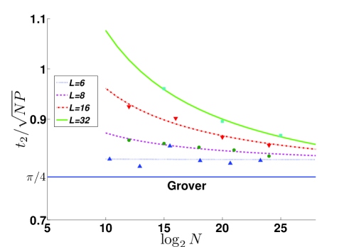
Figure 9: (Color online) $t_{2}/\sqrt{NP}$ as a function of the database size for different lattice sizes. The points are the data for $t_{1}=3$, and the curves are the fits $(t_{2}/\sqrt{NP})=a_{l}+(b_{l}/d)$. Also shown is the limiting value corresponding to Grover’s optimal algorithm.

The fit parameters for the three different optimised $s$-$t_{1}$ pairs are listed in Table III. They support our earlier scaling observations: $d_{1}$ close to $-1$ means that $P$ scales roughly as $2^{-d}$, and $d_{2}$ close to $-0.5$ means that $t_{2}$ scales roughly as $\sqrt{N/2^{d}}$. Interpreting Grover’s algorithm as the $d\rightarrow\infty$ limit of the spatial search algorithm, we expect $c_{3}$ to be close to $\pi/4$. It turns out to be somewhat smaller, but is not very accurately determined due to sizable correction from $d_{3}$ for the values of $d$ that we have. We believe that simulations for larger lattice sizes and higher dimensions can remedy this problem.

To look at our data in a different manner, we analyse the scaling behaviour of $t_{2}/\sqrt{NP}$ as a function of the database size. In Fig.9, we plot a subset of the data, illustrating how $t_{2}/\sqrt{NP}$ behaves for fixed lattice size $L$ when the database size is changed by changing $d$. The approach to the asymptotic behaviour is particularly clear in this form, with $t_{2}/\sqrt{NP}$ decreasing toward $\pi/4$ as the database size increases. It is also obvious that, for fixed $N$, our algorithm improves in efficiency with decreasing $L$ (or equivalently with increasing $d$). This is a consequence of the increase in the number of neighbours of a vertex with increasing $d$. An important implication is that, given a database of size $N$, it is best to implement the algorithm using the smallest $L$ (and hence the largest $d$) available. For our staggered fermion implementation of the Dirac operator, $L$ has to be even, and the smallest $L$ possible is $4$. Because of small values of $d$ that we have worked with, and discrete nature of $t_{2}$, our data for $L=4$ do not show smooth asymptotic behaviour. We therefore omitted $L=4$ from our analysis, and our best results are for $L=6$.

We can fit the data reasonably well as

$${t_{2}\over\sqrt{NP}}=a_{l}+{b_{l}\over d}~{}.$$ (29)

The fit parameters for the three different optimised $s$-$t_{1}$ pairs are listed in Table IV. We note that $a_{l}$ is close to $\pi/4$ when data for $d>6$ are available, but it cannot be accurately determined using data for small $d$ only due to sizable corrections from $b_{l}$.

Table 4: Fit parameters for $t_{2}/\sqrt{NP}$ vs. $d$ at fixed $L$.

$s$	$t_{1}$	$L$	Fitted $d$	$a_{l}$	$b_{l}$	Error
0.9539	2	6	5,6,7,8,9	0.766	$-$0.551	1.06$\times 10^{-2}$
		8	4,5,6,7,8	0.805	$-$0.293	5.31$\times 10^{-4}$
		16	3,4,5,6	0.663	$-$1.132	1.73$\times 10^{-2}$
		32	3,4,5	0.625	$-$1.304	5.77$\times 10^{-3}$
$1/\sqrt{2}$	3	6	4,5,6,7,8,9	0.819	$-$0.006	1.28$\times 10^{-2}$
		8	4,5,6,7,8	0.803	$-$0.234	3.28$\times 10^{-3}$
		16	3,4,5,6	0.773	$-$0.471	6.46$\times 10^{-3}$
		32	3,4,5	0.724	$-$0.705	3.23$\times 10^{-3}$
0.5410	4	6	4,5,6,7,8,9	0.837	$-$0.092	1.35$\times 10^{-2}$
		8	4,5,6,7,8	0.791	$-$0.272	3.79$\times 10^{-3}$
		16	3,4,5,6	0.767	$-$0.450	1.29$\times 10^{-3}$
		32	3,4,5	0.711	$-$0.726	1.13$\times 10^{-3}$

IV Results for MultipleMarked Vertices

We also carried out a few simulations of spatial search with more than one marked vertex. The change from the single marked vertex algorithm is that the search oracle now flips the sign of amplitudes at several distinct vertices, say $M$. To see clear patterns in the results, we needed to keep the marked vertices well separated and avoid interference effects.

Table 5: Spatial search results for multiple marked vertices in $d=3$.

$s$	$t_{1}$	$M$	Marked vertices	$P$	$t_{2}$
$1/\sqrt{2}$	3	1	(32,32,32)	0.09829	161
		2	(0,32,32), (32,32,32)	0.04919, 0.04919	112, 112
			(0,32,33), (32,32,32)	0.09868, 0.09790	161, 161
		3	(0,0,0), (16,16,16), (32,32,32)	0.03530, 0.03264, 0.03082	94, 92, 92
			(0,0,1), (16,16,16), (32,32,32)	0.09380, 0.05590, 0.04507	161, 117, 109
			(0,0,1), (16,16,16), (33,32,32)	0.09298, 0.09838, 0.10347	157, 161, 162

With the staggered fermion implementation of the Dirac operator, it matters whether the marked vertices belong to the same corner of the elementary hypercube or to different corners. So we considered various hypercube locations for the marked vertices. In Table V, we compare our illustrative results for two and three marked vertices with those for a single marked vertex. The values for peak probability $P$ and corresponding time $t_{2}$ were obtained with $s=1/\sqrt{2}$ and $t_{1}=3$ on a $64^{3}$ lattice.

When the marked vertices belong to the same corner of the elementary hypercube (e.g. (0,32,32) and (32,32,32)), they involve the same degree of freedom. In that case, we observe that $P$ decreases by a factor of $M$ and $t_{2}$ decreases by a factor of $\sqrt{M}$. On the other hand, when the marked vertices belong to different corners of the elementary hypercube (e.g. (0,32,33) and (32,32,32)), they involve different degrees of freedom. In that case, we find that $P$ and $t_{2}$ are more or less the same as for the single marked vertex case. This pattern is also followed when some marked vertices are at the same corner of the elementary hypercube and some at different corners.

We can infer the following equipartition rule from these observations. A fixed peak probability (upper bounded by $2^{-d}$) is available for each corner degree of freedom of the elementary hypercube. Multiple marked vertices corresponding to the same degree of freedom share this peak probability equally, while different degrees of freedom evolve independently of each other. Apart from this caveat, the dependence of $t_{2}$ on $M$ for our spatial search algorithm is the same as in the case of Grover’s algorithm, i.e. proportional to $\sqrt{N/M}$.

V Summary

We have formulated the spatial search problem using staggered fermion discretisation of the Dirac operator on a hypercubic lattice in arbitrary dimension. Our search strategy, Eq.(19), mimics that of Grover’s algorithm. The locality restriction on the walk operator becomes less and less relevant as the dimensionality of the space increases, and we expect to reach the optimal scaling behaviour of Grover’s algorithm as $d\rightarrow\infty$.

We have verified our theoretical expectations by numerical simulations of the algorithm for $d=3$ to $d=9$. We clearly demonstrate the approach to the $d\rightarrow\infty$ limit, and find that even for $d=3$ our algorithm is only $25\%$ less efficient. From a computational cost point of view, for a fixed database size $N$, our best parameters are $t_{1}=2$ and the largest $d$ available. With the staggered fermion implementation, our algorithm works in total Hilbert space dimension $N$. That is a big reduction from the total Hilbert dimension $2^{d}N$ required by the algorithms that use coin or internal degrees of freedom (for the best $d=\Theta(\ln N)$, $2^{d}=O(N)$ is substantial), and makes our exercise worthwhile.

References

- (1) L.K. Grover, Proceedings of STOC’96 (ACM Press, New York, 1996), p. 212, arXiv:quant-ph/9605043.
- (2) N. Shenvi, J. Kempe and K. Birgitta Whaley, Phys. Rev. A67 (2003) 052307, arXiv:quant-ph/0210064.
- (3) A. Ambainis, J. Kempe and A. Rivosh, Proceedings of ACM-SIAM SODA’05 (ACM Press, New York, 2005), p. 1099, arXiv:quant-ph/0402107.
- (4) A.M. Childs and J. Goldstone, Phys. Rev. A70 (2004) 042312, arXiv:quant-ph/0405120.
- (5) A. Tulsi, Phys. Rev. A78 (2008) 012310, arXiv:0801.0497.
- (6) B. Hein and G. Tanner, J. Phys. A42 (2009) 085303, arXiv:0906.3094.
- (7) G. Abal, R. Donangelo, F.L. Marquezino and R. Portugal, Math. Struct. Comp. Sci. (2010), to appear, arXiv:1001.1139.
- (8) L.K. Grover, Pramana 56 (2001) 333, arXiv:quant-ph/0109116.
- (9) Y. Aharonov, L. Davidovich and N. Zagury, Phys. Rev. A48 (1993) 1687.
- (10) J. Kempe, Contemporary Physics 44 (2003) 307, arXiv:quant-ph/0303081.
- (11) L. Susskind, Phys. Rev. D16 (1977) 3031.
- (12) A. Patel, K.S. Raghunathan and Md.A. Rahaman, Phys. Rev. A82 (2010) 032331, arXiv:1003.5564.
- (13) A. Patel, K.S. Raghunathan and P. Rungta, Phys. Rev. A71 (2005) 032347, arXiv:quant-ph/0405128.
- (14) This is in spite of the fact that Dirac spinors require components in dimensions. For example, in , a Rubik’s cube can have the central cube labeled “o” and the eight corner cubes labeled “e”.
- (15) A. Patel, K.S. Raghunathan and P. Rungta, Proceedings of the Workshop on Quantum Information, Computation and Communication (QICC-2005), IIT Kharagpur, India, (Allied Publishers, 2006), p. 41, arXiv:quant-ph/0506221.
- (16) G. Brassard, P. Hoyer, M. Mosca and A. Tapp, in Quantum Computation and Information, AMS Contemporary Mathematics Series Vol. 305, eds. S.J. Lomonaco and H.E. Brandt (AMS, Providence, 2002), p. 53, arXiv:quant-ph/0005055.
- (17) C. Zalka, Phys. Rev. A60 (1999) 2746, arXiv:quant-ph/9711070.
- (18) C. Bennett, E. Bernstein, G. Brassard and U. Vazirani, SIAM J. Comput. 26 (1997) 1510, arXiv:quant-ph/9701001.