Decoding by Sampling: A Randomized Lattice Algorithm for Bounded Distance Decoding

Abstract

Despite its reduced complexity, lattice reduction-aided decoding exhibits a widening gap to maximum-likelihood (ML) performance as the dimension increases. To improve its performance, this paper presents randomized lattice decoding based on Klein’s sampling technique, which is a randomized version of Babai’s nearest plane algorithm (i.e., successive interference cancelation (SIC)). To find the closest lattice point, Klein’s algorithm is used to sample some lattice points and the closest among those samples is chosen. Lattice reduction increases the probability of finding the closest lattice point, and only needs to be run once during pre-processing. Further, the sampling can operate very efficiently in parallel. The technical contribution of this paper is two-fold: we analyze and optimize the decoding radius of sampling decoding resulting in better error performance than Klein’s original algorithm, and propose a very efficient implementation of random rounding. Of particular interest is that a fixed gain in the decoding radius compared to Babai’s decoding can be achieved at polynomial complexity. The proposed decoder is useful for moderate dimensions where sphere decoding becomes computationally intensive, while lattice reduction-aided decoding starts to suffer considerable loss. Simulation results demonstrate near-ML performance is achieved by a moderate number of samples, even if the dimension is as high as 32.

I INTRODUCTION

Decoding for the linear multi-input multi-output (MIMO) channel is a problem of high relevance in multi-antenna, cooperative and other multi-terminal communication systems. The computational complexity associated with maximum-likelihood (ML) decoding poses significant challenges for hardware implementation. When the codebook forms a lattice, ML decoding corresponds to solving the closest lattice vector problem (CVP). The worst-case complexity for solving the CVP optimally for generic lattices is non-deterministic polynomial-time (NP)-hard. The best CVP algorithms to date are Kannan’s [1] which has be shown to be of complexity $n^{n/2+o(n)}$ where $n$ is the lattice dimension (see [2]) and whose space requirement is polynomial in $n$, and the recent algorithm by Micciancio and Voulgaris [3] which has complexity $2^{O(n)}$ with respect to both time and space. In digital communications, a finite subset of the lattice is used due to the power constraint. ML decoding for a finite (or infinite) lattice can be realized efficiently by sphere decoding [4, 5, 6], whose average complexity grows exponentially with $n$ for any fixed SNR [7]. This limits sphere decoding to low dimensions in practical applications. The decoding complexity is especially felt in coded systems. For instance, to decode the $4\times 4$ perfect code [8] using the 64-QAM constellation, one has to search in a 32-dimensional (real-valued) lattice; from [7], sphere decoding requires a complexity of $64^{32\gamma}$ with some $\gamma\in\left(0,1\right]$, which could be huge. Although some fast-decodable codes have been proposed recently [9], the decoding still relies on sphere decoding.

Thus, we often have to resort to approximate solutions. The problem of solving CVP approximately was first addressed by Babai in [10], which in essence applies zero-forcing (ZF) or successive interference cancelation (SIC) on a reduced lattice. This technique is often referred to as lattice-reduction-aided decoding [11, 12]. It is known that ZF or minimum mean square error (MMSE) detection aided by Lenstra, Lenstra and Lovász (LLL) reduction achieves full diversity in uncoded MIMO fading channels [13, 14] and that lattice-reduction-aided decoding has a performance gap to (infinite) lattice decoding depending on the dimension $n$ only [15]. It was further shown in [16] that MMSE-based lattice-reduction aided decoding achieves the optimal diversity and spatial multiplexing tradeoff. In [17], it was shown that Babai’s decoding using MMSE can provide near-ML performance for small-size MIMO systems. However, the analysis in [15] revealed a widening gap to ML decoding. In particular, both the worst-case bound and experimental gap for LLL reduction are exponential with dimension $n$ (or linear with $n$ if measured in dB).

In this work, we present sampling decoding to narrow down the gap between lattice-reduction-aided SIC and sphere decoding. We use Klein’s sampling algorithm [18], which is a randomized version of Babai’s nearest plane algorithm (i.e., SIC). The core of Klein’s algorithm is randomized rounding which generalizes the standard rounding by not necessarily rounding to the nearest integer. Thus far, Klein’s algorithm has mostly remained a theoretic tool in the lattice literature, while we are unaware of any experimental work for Klein’s algorithm in the MIMO literature. In this paper, we sample some lattice points by using Klein’s algorithm and choose the closest from the list of sampled lattice points. By varying the list size $K$, it enjoys a flexible tradeoff between complexity and performance. Klein applied his algorithm to find the closest lattice point only when it is very close to the input vector: this technique is known as bounded-distance decoding (BDD) in coding literature. The performance of BDD is best captured by the correct decoding radius (or simply decoding radius), which is defined as the radius of a sphere centered at the lattice point within which decoding is guaranteed to be correct.

The technical contribution of this paper is two-fold: we analyze and optimize the performance of sampling decoding which leads to improved error performance than the original Klein algorithm, and propose a very efficient implementation of Klein’s random rounding, resulting in reduced decoding complexity. In particular, we show that sampling decoding can achieve any fixed gain in the decoding radius (over Babai’s decoding) at polynomial complexity. Although a fixed gain is asymptotically vanishing with respect to the exponential proximity factor of LLL reduction, it could be significant for the dimensions of interest in the practice of MIMO. In particular, simulation results demonstrate that near-ML performance is achieved by a moderate number of samples for dimension up to 32. The performance-complexity tradeoff of sampling decoding is comparable to that of the new decoding algorithms proposed in [19, 20] very recently. A byproduct is that boundary errors for finite constellations can be partially compensated if we discard the samples falling outside of the constellation.

Sampling decoding distinguishes itself from previous list-based detectors [21, 22, 23, 24, 25] in several ways. Firstly, the way it builds its list is distinct. More precisely, it randomly samples lattice points with a discrete Gaussian distribution centered at the received signal and returns the closest among them. A salient feature is that it will sample a closer lattice point with higher probability. Hence, our sampling decoding is more likely to find the closest lattice point than [24] where a list of candidate lattice points is built in the vicinity of the SIC output point. Secondly, the expensive lattice reduction is only performed once during pre-processing. In [22], a bank of $2n$ parallel lattice reduction-aided detectors was used. The coset-based lattice detection scheme in [23], as well as the iterative lattice reduction detection scheme [25], also needs lattice reduction many times. Thirdly, sampling decoding enjoys a proven gain given the list size $K$; all previous schemes might be viewed as various heuristics apparently without such proven gains. Note that list-based detectors (including our algorithm) may prove useful in the context of incremental lattice decoding [26], as it provides a fall-back strategy when SIC starts failing due to the variation of the lattice.

It is worth mentioning that Klein’s sampling technique is emerging as a fundamental building block in a number of new lattice algorithms [27, 28]. Thus, our analysis and implementation may benefit those algorithms as well.

The paper is organized as follows: Section II presents the transmission model and lattice decoding, followed by a description of Klein’s sampling algorithm in Section III. In Section IV the fine-tuning and analysis of sampling decoding is given, and the efficient implementation and extensions to complex-valued systems, MMSE and soft-output decoding are proposed in Section V. Section VI evaluates the performance and complexity by computer simulation. Some concluding remarks are offered in Section VII.

Notation: Matrices and column vectors are denoted by upper and lowercase boldface letters, and the transpose, inverse, pseudoinverse of a matrix $\mathbf{B}$ by $\mathbf{B}^{T}$, $\mathbf{B}^{-1}$, and $\mathbf{B}^{\dagger}$, respectively. $\mathbf{I}$ is the identity matrix. We denote $\mathbf{b}_{i}$ for the $i$-th column of matrix $\mathbf{B}$, $b_{i,j}$ for the entry in the $i$-th row and $j$-th column of the matrix $\mathbf{B}$, and $b_{i}$ for the $i$-th entry in vector $\mathbf{b}$. Vec$(\mathbf{B})$ stands for the column-by-column vectorization of the matrices $\mathbf{B}$. The inner product in the Euclidean space between vectors $\mathbf{u}$ and $\mathbf{v}$ is defined as $\langle\mathbf{u},\mathbf{v}\rangle=\mathbf{u}^{T}\mathbf{v}$, and the Euclidean length $\|\mathbf{u}\|=\sqrt{\langle\mathbf{u},\mathbf{u}\rangle}$. Kronecker product of matrix $\mathbf{A}$ and $\mathbf{B}$ is written as $\mathbf{A}\otimes\mathbf{B}$. $\lceil x\rfloor$ rounds to a closest integer, while $\lfloor x\rfloor$ to the closest integer smaller than or equal to $x$ and $\left\lceil x\right\rceil$ to the closest integer larger than or equal to $x$. The $\mathfrak{\Re}$ and $\mathfrak{\Im}$ prefixes denote the real and imaginary parts. A circularly symmetric complex Gaussian random variable $x$ with variance $\sigma^{2}$ is defined as $x\backsim\mathcal{CN}\left(0,\sigma^{2}\right)$. We write $\triangleq$ for equality in definition. We use the standard asymptotic notation $f\left(x\right)=O\left(g\left(x\right)\right)$ when $\lim\sup_{x\rightarrow\infty}|f(x)/g(x)|<\infty$ , $f\left(x\right)=\Omega\left(g\left(x\right)\right)$ when $\lim\sup_{x\rightarrow\infty}|g(x)/f(x)|<\infty$, and $f\left(x\right)=o\left(g\left(x\right)\right)$ when $\lim\sup_{x\rightarrow\infty}|f(x)/g(x)|=0$ . Finally, in this paper, the computational complexity is measured by the number of arithmetic operations.

II LATTICE CODING AND DECODING

Consider an $n_{T}\times n_{R}$ flat-fading MIMO system model consisting of $n_{T}$ transmitters and $n_{R}$ receivers

$$\mathbf{Y=HX+N},$$ (1)

where $\mathbf{X}\in\mathbb{C}^{n_{T}\times T}$, $\mathbf{Y}$, $\mathbf{N}\in\mathbb{C}^{n_{R}\times T}$ of block length $T$ denote the channel input, output and noise, respectively, and $\mathbf{H}\in\mathbb{C}^{n_{R}\times n_{T}}$ is the $n_{R}\times n_{T}$ full-rank channel gain matrix with $n_{R}\geq n_{T}$, all of its elements are i.i.d. complex Gaussian random variables $\mathcal{CN}\left(0,1\right)$. The entries of $\mathbf{N}$ are i.i.d. complex Gaussian with variance $\sigma^{2}$ each. The codewords $\mathbf{X}$ satisfy the average power constraint $E[\|\mathbf{X}\|^{2}_{\text{F}}/T]=1$. Hence, the signal-to-noise ratio (SNR) at each receive antenna is $1/\sigma^{2}$.

When a lattice space-time block code is employed, the codeword $\mathbf{X}$ is obtained by forming a $n_{T}\times T$ matrix from vector $\mathbf{s}\in\mathbb{C}^{n_{T}T}$, where $\mathbf{s}$ is obtained by multiplying $n_{T}T\times 1$ QAM vector $\mathbf{x}$ by the $n_{T}T\times n_{T}T$ generator matrix $\mathbf{G}$ of the encoding lattice, i.e., $\mathbf{s}=\mathbf{Gx}$. By column-by-column vectorization of the matrices $\mathbf{Y}$ and $\mathbf{N}$ in (1), i.e., $\mathbf{y}=\text{Vec}(\mathbf{Y})$ and $\mathbf{n}=\text{Vec}(\mathbf{N})$, the received signal at the destination can be expressed as

$$\mathbf{y=}\left(\mathbf{I}_{T}\otimes\mathbf{H}\right)\mathbf{Gx+n}\text{.}$$ (2)

When $T=1$ and $\mathbf{G=I}_{n_{T}}$, (2) reduces to the model for uncoded MIMO communication $\mathbf{y}=\mathbf{Hx}+\mathbf{n}$. Further, we can equivalently write

$$\left[\begin{array}[]{c}\mathfrak{\Re}\mathbf{y}\\ \mathfrak{\Im}\mathbf{y}\end{array}\right]=\left[\begin{array}[]{cc}\mathfrak{\Re}\mathbf{H}&-\mathfrak{\Im}\mathbf{H}\\ \mathfrak{\Im}\mathbf{H}&\mathfrak{\Re}\mathbf{H}\end{array}\right]\left[\begin{array}[]{c}\mathfrak{\Re}\mathbf{x}\\ \mathfrak{\Im}\mathbf{x}\end{array}\right]+\left[\begin{array}[]{c}\mathfrak{\Re}\mathbf{n}\\ \mathfrak{\Im}\mathbf{n}\end{array}\right],$$ (3)

which gives an equivalent $2n_{T}\times 2n_{R}$ real-valued model. We can also obtain an equivalent $2n_{T}T\times 2n_{R}T$ real model for coded MIMO like (3). The QAM constellations $\mathcal{C}$ can be interpreted as the shift and scaled version of a finite subset $\mathcal{A}^{n_{T}}$ of the integer lattice $\mathbb{Z}^{n_{T}}$, i.e., $\mathcal{C}=a(\mathcal{A}^{n_{T}}+[1/2,...,1/2]^{T})$, where the factor $a$ arises from energy normalization. For example, we have $\mathcal{A}^{n_{T}}=\{-\sqrt{M}/2,...,\sqrt{M}/2-1\}$ for M-QAM signalling.

Therefore, with scaling and shifting, we consider the canonical $n\times m$ ($m\geq n$) real-valued MIMO system model

$$\mathbf{y}=\mathbf{Bx}+\mathbf{n}$$ (4)

where $\mathbf{B}\in\mathbb{R}^{m\times n}$, given by the real-valued equivalent of $\left(\mathbf{I}_{T}\otimes\mathbf{H}\right)\mathbf{G}$, can be interpreted as the basis matrix of the decoding lattice. Obviously, $n=2n_{T}T$ and $m=2n_{R}T$. The data vector $\mathbf{x}$ is drawn from a finite subset $\mathcal{A}^{n}$ to satisfy the power constraint.

A lattice in the $m$-dimensional Euclidean space $\mathbb{R}^{m}$ is generated as the integer linear combination of the set of linearly independent vectors [29, 30]:

$$\mathcal{L\triangleq L}\left(\mathbf{B}\right)\mathbf{=}\left\{\sum_{i=1}^{n}x_{i}\mathbf{b}_{i}\left|x_{i}\in\mathbb{Z}\text{, }i=1,\ldots n\right.\right\},$$ (5)

where $\mathbb{Z}$ is the set of integers, and $\mathbf{B=}\left[\mathbf{b}_{1}\cdots\mathbf{b}_{n}\right]$ represents a basis of the lattice $\mathcal{L}$. In the matrix form, $\mathcal{L=}\left\{\mathbf{Bx}\text{ : }\mathbf{x\in}\text{ }\mathbb{Z}^{n}\right\}$. The lattice has infinitely many different bases other than $\mathbf{B}$. In general, a matrix $\mathbf{{B^{\prime}}=BU}$, where $\mathbf{U}$ is an unimodular matrix, i.e., $\det\mathbf{U=\pm}1$ and all elements of $\mathbf{U}$ are integers, is also a basis of $\mathcal{L}$.

Since the vector $\mathbf{Bx}$ can be viewed as a lattice point, MIMO decoding can be formulated as a lattice decoding problem. The ML decoder computes

$$\mathbf{\hat{x}}=\arg\min_{\mathbf{x}\in\mathcal{A}^{n}}\|\mathbf{y}-\mathbf{Bx}\|^{2}.$$ (6)

which amounts to solving a closest-vector problem (CVP) in a finite subset of lattice $\mathcal{L}$. ML decoding may be accomplished by the sphere decoding. However, the expected complexity of sphere decoding is exponential for fixed SNR [7].

A promising approach to reducing the computational complexity of sphere decoding is to relax the finite lattice to the infinite lattice and to solve

$$\mathbf{\hat{x}}=\arg\min_{\mathbf{x}\in\mathbb{Z}^{n}}\|\mathbf{y}-\mathbf{Bx}\|^{2}.$$ (7)

which could benefit from lattice reduction. This technique is sometimes referred to as infinite lattice decoding (ILD). The downside is that the found lattice point will not necessarily be a valid point in the constellation.

This search can be carried out more efficiently by lattice reduction-aided decoding [12]. The basic idea behind this is to use lattice reduction in conjunction with traditional low-complexity decoders. With lattice reduction, the basis $\mathbf{B}$ is transformed into a new basis consisting of roughly orthogonal vectors

$$\mathbf{B^{\prime}}=\mathbf{BU}$$ (8)

where $\mathbf{U}$ is a unimodular matrix. Indeed, we have the equivalent channel model

$$\mathbf{y}=\mathbf{B^{\prime}U}^{-1}\mathbf{x}+\mathbf{n}=\mathbf{B^{\prime}x^{\prime}}+\mathbf{n},\quad\mathbf{x^{\prime}}=\mathbf{U^{-1}x}.$$

Then conventional decoders (ZF or SIC) are applied on the reduced basis. This estimate is then transformed back into $\mathbf{\hat{x}}=\mathbf{U\hat{x}^{\prime}}$. Since the equivalent channel is much more likely to be well-conditioned, the effect of noise enhancement will be moderated. Again, as the resulting estimate $\mathbf{\hat{x}}$ is not necessarily in $\mathcal{A}^{n}$, remapping of $\mathbf{\hat{x}}$ onto the finite lattice $\mathcal{A}^{n}$ is required whenever $\mathbf{\hat{x}}\notin\mathcal{A}^{n}$.

Babai pre-processed the basis with lattice reduction, then applied either the rounding off (i.e., ZF) or nearest plane algorithm (i.e., SIC) [10]. For SIC, one performs the QR decomposition $\mathbf{B}=\mathbf{QR}$, where $\mathbf{Q}$ has orthogonal columns and $\mathbf{R}$ is an upper triangular matrix with positive diagonal elements [31]. Multiplying (4) on the left with $\mathbf{Q^{\dagger}}$ we have

$$\mathbf{y}^{\prime}=\mathbf{Q^{\dagger}y}=\mathbf{Rx}+\mathbf{n}^{\prime}.$$ (9)

In SIC, the last symbol $x_{n}$ is estimated first as $\hat{x}_{n}=\lceil y_{n}^{\prime}/r_{n,n}\rfloor$. Then the estimate is substituted to remove the interference term in $y_{n-1}^{\prime}$ when $x_{n-1}$ is being estimated. The procedure is continued until the first symbol is detected. That is, we have the following recursion:

$$\hat{x}_{i}=\left\lceil\frac{y_{i}^{\prime}-\sum_{j=i+1}^{n}r_{i,j}\hat{x}_{j}}{r_{i,i}}\right\rfloor$$ (10)

for $i=n,n-1,...,1$.

Let $\mathbf{\hat{b}}_{1}$,…,$\mathbf{\hat{b}}_{n}$ be the Gram-Schmidt vectors where $\mathbf{\hat{b}}_{i}$ is the projection of $\mathbf{b}_{i}$ orthogonal to the vector space generated by $\mathbf{b}_{1}$,…,$\mathbf{b}_{i-1}$. These are the vectors found by the Gram-Schmidt algorithm for orthogonalization. Gram-Schmidt orthogonalization is closely related to QR decomposition. More precisely, one has the relations $\mathbf{\hat{b}}_{i}=$ $r_{i,i}\cdot\mathbf{q}_{i}$, where $\mathbf{q}_{i}$ is the $i$-th column of $\mathbf{Q}$. It is known that SIC finds the closest vector if the distance from input vector $\mathbf{y}$ to the lattice $\mathcal{L}$ is less than half the length of the shortest Gram-Schmidt vector. In other words, the correct decoding radius for SIC is given by

$$R_{\text{SIC}}=\frac{1}{2}\min_{1\leq i\leq n}\|\mathbf{\hat{b}}_{i}\|=\frac{1}{2}\min_{1\leq i\leq n}r_{i,i}.$$ (11)

The proximity factor defined in [15] quantifies the worst-case loss in the correct decoding radius relative to ILD

$$F_{\text{SIC}}\triangleq\frac{R_{\text{ILD}}^{2}}{R_{\text{SIC}}^{2}},$$ (12)

where the correct decoding radius for ILD is $R_{\text{ILD}}=\lambda_{1}/2$ ($\lambda_{1}$ is the minimum distance, or the length of a shortest nonzero vector of the lattice $\mathcal{L}$) and showed that under LLL reduction

$$F_{\text{SIC}}\leq\beta^{n-1},\quad\beta=\left(\delta-1/4\right)^{-1}$$ (13)

where $1/4<\delta\leq 1$ is a parameter associated with LLL reduction [32]. Note that the average-case gap for random bases $\mathbf{B}$ is smaller. Yet it was observed experimentally in [33, 15] that the average-case proximity (or approximation) factor remains exponential for random lattices. Meanwhile, if one applies dual KZ reduction, then [15]

$$F_{\text{SIC}}\leq n^{2}.$$ (14)

Again, the worst-case loss relative to ILD widens with $n$.

These finite proximity factors imply that lattice reduction-aided SIC is an instance of BDD. More precisely, the $1/(2\gamma)$-BDD problem is to find the closest lattice point given that the distance between input $\mathbf{y}$ and lattice $\mathcal{L}$ is less than $\lambda_{1}/(2\gamma)$. It is easy to see that a decoding algorithm with proximity factor $F$ corresponds to $1/(2\sqrt{F})$-BDD.

III SAMPLING DECODING

Klein [18] proposed a randomized BDD algorithm that increased the correct decoding radius to

$$R_{\text{Klein}}=k\min_{1\leq i\leq n}r_{i,i}.$$

For the algorithm to be useful, the parameter $k$ should fall into the range $1/2<k<\sqrt{n/2}$; in other regions Babai and Kannan’s algorithms would be more efficient. Its complexity is $n^{k^{2}+O(1)}$ which for fixed $k$ is polynomial in $n$ as $n\rightarrow\infty$.

In essence, Klein’s algorithm is a randomized version of SIC, where standard rounding in SIC is replaced by randomized rounding. Klein described his randomized algorithm in the recursive form. Here, we rewrite it into the non-recursive form more familiar to the communications community. It is summarized by the pseudocode of the function Rand_SIC${}_{A}\left(\mathbf{y}^{\prime}\right)$ in Table I. We assume that the pre-processing of (9) has been done, hence the input $\mathbf{y}^{\prime}=\mathbf{Q^{\dagger}y}$ rather than $\mathbf{y}$. This will reduce the complexity since we will call it many times. The important parameter $A$ determines the amount of randomness, and Klein suggested $A=\log n/\min_{i}r_{i,i}^{2}$.

TABLE I: Pseudocode for the randomized SIC in sequential form

Function Rand_SIC${}_{A}\left(\mathbf{y^{\prime}}\right)$
1: for $i=n$ to $1$ do
2:   $c_{i}\longleftarrow Ar_{i,i}^{2}$
3:   $\hat{x}_{i}\longleftarrow$ Rand_Round${}_{c_{i}}\left(({y}_{i}^{\prime}-\sum_{j=i+1}^{n}r_{i,j}\hat{x}_{j})/r_{i,i}\right)$
4: end for
5: return $\mathbf{\hat{x}}$

The randomized SIC randomly samples a lattice point $\mathbf{z}$ that is close to $\mathbf{y}$. To obtain the closest lattice point, one calls Rand_SIC $K$ times and chooses the closest among those lattice points returned, with a sufficiently large $K$. The function Rand_Round${}_{c}(r)$ rounds $r$ randomly to an integer $Q$ according to the following discrete Gaussian distribution [18]

$$P(Q=q)=e^{-c(r-q)^{2}}/s,\quad s=\sum_{q=-\infty}^{\infty}{e^{-c(r-q)^{2}}}.$$ (15)

If $c$ is large, Rand_Round reduces to standard rounding (i.e., decision is confident); if $c$ is small, it makes a guess (i.e., decision is unconfident).

Lemma 1

([18]) $s\leq s(c)\triangleq\sum_{i\geq 0}{e^{-ci^{2}}+e^{-c(1+i)^{2}}.}$

The proof of the lemma was given in [18] and is omitted here. The next lemma provides a lower bound on the probability that Klein’s algorithm or Rand_SIC returns $\mathbf{z}\in\mathcal{L}$.

Lemma 2

([18]) Let $\mathbf{z}$ be a vector in $\mathcal{L}\left(\mathbf{B}\right)$ and $\mathbf{y}$ be a vector in $\mathbb{R}^{m}$. The probability that Klein’s algorithm or Rand_SIC return $\mathbf{z}$ is bounded by

$$P(\mathbf{z})\geq\frac{1}{\prod_{i=1}^{n}{s(Ar_{i,i}^{2})}}e^{-A\|\mathbf{y}-\mathbf{z}\|^{2}}.$$ (16)

Proof:

The proof of the lemma was given in [18] for the recursive version of Klein’s algorithm. Here, we give a more straightforward proof for Rand_SIC. Let $\mathbf{z=}\xi_{1}\mathbf{b}_{1}+\mathbf{\ldots}+\xi_{n}\mathbf{b}_{n}=\mathbf{B\xi}\in\mathcal{L},\xi_{i}\in\mathbb{Z}$ and consider the invocation of Rand_SIC${}_{A}\left(\mathbf{y^{\prime}}\right)$. Using Lemma 1 and (15), the probability of $x_{i}=\xi_{i}$ is at least

$$\begin{split}&\frac{1}{{s(Ar_{i,i}^{2})}}e^{-Ar_{i,i}^{2}\left(({y}_{i}^{\prime}-\sum_{j=i+1}^{n}r_{i,j}\xi_{j})/r_{i,i}\right){{{}^{2}}}}\\ =&\frac{1}{{s(Ar_{i,i}^{2})}}e^{-A\left({y}_{i}^{\prime}-\sum_{j=i+1}^{n}r_{i,j}\xi_{j}\right){{{}^{2}}}}.\end{split}$$ (17)

By multiplying these $n$ probabilities, we obtain a lower bound on the probability that Rand_SIC returns $\mathbf{z}$

$$\begin{split}P\left(\mathbf{z}\right)&\geq\frac{1}{\prod_{i\leq n}{s(Ar_{i,i}^{2})}}e^{-A\sum_{i=1}^{n}\left({y}_{i}^{\prime}-\sum_{j=i+1}^{n}r_{i,j}\xi_{j}\right)^{2}}\\ &=\frac{1}{\prod_{i\leq n}{s(Ar_{i,i}^{2})}}e^{-A\|\mathbf{y}^{\prime}-\mathbf{R\xi}\|^{2}}\\ &\geq\frac{1}{\prod_{i\leq n}{s(Ar_{i,i}^{2})}}e^{-A\|\mathbf{y}-\mathbf{B\xi}\|^{2}}.\end{split}$$ (18)

So the probability is as stated in Lemma 2.    

A salient feature of (16) is that the closest lattice point is the most likely to be sampled. In particular, the lower bound resembles the Gaussian distribution. The closer $\mathbf{z}$ is to $\mathbf{y}$, the more likely it will be sampled. Klein showed that when $A=\log n/\min_{i}r_{i,i}^{2}$, the probability of returning $\mathbf{z}\in\mathcal{L}$ is

$$\Omega(n^{-\|\mathbf{y}-\mathbf{z}\|^{2}/\min_{i}r_{i,i}^{2}}).$$ (19)

The significance of lattice reduction can be seen here, as increasing $\min_{i}r_{i,i}^{2}$ will increase the probability lower bound (19).

As lattice reduction-aided decoding normally ignores the boundary of the constellation, the samples returned by Rand_SIC${}_{A}(\mathbf{y^{\prime}})$ come from an extended version of the original constellation. We discard those samples that happen to lie outside the boundary of the original constellation and choose the closest among the rest lattice points. When no lattice points within the boundary are found, we simply remap the closest one back to the constellation by “hard-limiting”, i.e., remap $\hat{x}_{i}$ to one of the two boundary integers that is closer to it.

Remark: A natural questions is whether a randomized version of ZF exists. The answer is yes. This can be done by applying random rounding in ZF. However, since its performance is not as good as randomized SIC, it will not be considered in this paper.

IV ANALYSIS AND OPTIMIZATION

The list size $K$ is often limited in communications. Given $K$, the parameter $A$ has a profound impact on the decoding performance, and Klein’s choice $A=\log n/\min_{i}r_{i,i}^{2}$ is not necessarily optimum. In this Section, we want to answer the following questions about randomized lattice decoding:

• Given $K$, what is the optimum value of $A$?

• Given $K$ and associated optimum $A$, how much is the gain in decoding performance?

• What is the limit of sampling decoding?

Indeed, there exists an optimum value of $A$ when $K$ is finite, since $A\rightarrow 0$ means uniform sampling of the entire lattice while $A\rightarrow\infty$ means Babai’s algorithm. We shall present an approximate analysis of optimum $A$ for a given $K$ in the sense of maximizing the correct decoding radius, and then estimate the decoding gain over Babai’s algorithm. The analysis is not exact since it is based on the correct decoding radius only; nonetheless, it captures the key aspect of the decoding performance and can serve as a useful guideline to determine the parameters in practical implementation of Klein’s algorithm.

IV-A Optimum Parameter $A$

We investigate the effect of parameter $A$ on the probability Rand_SIC returns $\mathbf{z}\in\mathcal{L}$. Let $A=\log\rho/\min_{i}r_{i,i}^{2}$, where ${\rho>1}$ (so that $A>0$). Then $\rho$ is the parameter to be optimized. Since $c_{i}=Ar_{i,i}^{2}\geq\log\rho$, we have the following bound for $s(c_{i})$:

$$s(c_{i}) = \sum_{i\geq 0}{e^{-c_{i}i^{2}}+e^{-c_{i}(1+i)^{2}}}$$ (20)

$$\leq \sum_{i\geq 0}\rho{{}^{-i^{2}}+\rho^{-(1+i)^{2}}}$$

$$= 1+2\left({\rho}^{-1}+{\rho}^{-4}+{\rho}^{-9}+\ldots\right)$$

$$< 1+2/{\rho+2\rho}^{-4}/\left(1-{\rho}^{-5}\right).$$

Hence

$$\prod_{i=1}^{n}{s(c_{i})} {<} \left(\exp\left(2/{\rho}+{2\rho}^{-4}/\left(1-{\rho}^{-5}\right)\right)\right)^{n}$$ (21)

$$= e^{\frac{2n}{\rho}(1+{g(\rho)})}\text{,}$$

where ${g(\rho)=\rho}^{-3}/\left(1-{\rho}^{-5}\right)$. With this choice of parameter $A$, (16) can be bounded from below by

$$P(\mathbf{z})>e^{-\frac{2n}{\rho}(1+{g(\rho)})}\cdot\rho^{-\|\mathbf{y}-\mathbf{z}\|^{2}/\min_{i}r_{i,i}^{2}}.$$ (22)

Now, let $\mathbf{z}_{K}$ be a point in the lattice, with $P(\mathbf{z}_{K})>1/K$. With $K$ calls to Klein’s algorithm, the probability of missing $\mathbf{z}_{K}$ is not larger than $(1-1/K)^{K}<1/e$. By increasing the number of calls to $cK$ ($c\geq 1$ is a constant independent of $n$), we can make this missing probability smaller than $1/e^{c}$. The value of $c$ could be found by simulation, and $c=1$ is often enough. Therefore, any such lattice point $\mathbf{z}_{K}$ will be found with probability close to one. We assume that ${\rho}$ is not too small such that ${g(\rho)}$ is negligible. This is a rather weak condition: even $\rho\geq 2$ is sufficient. As will be seen later, this condition is indeed satisfied for our purpose. From (22), we obtain

$$e^{-\frac{2n}{\rho}}\cdot\rho^{-\|\mathbf{y}-\mathbf{z}_{K}\|^{2}/\min_{i}r_{i,i}^{2}}\approx\frac{1}{K}$$

$$\|\mathbf{y}-\mathbf{z}_{K}\|\approx\min_{i}r_{i,i}\cdot\sqrt{\log_{\rho}\left(Ke^{-2n/\rho}\right)}.$$ (23)

The sampling decoder will find the closest vector point almost surely if the distance from input vector $\mathbf{y}$ to the lattice is less than the right hand side of (23), since the probability of being sampled can only be higher than $1/K$. In this sense, the right hand side of (23) can be thought of as the decoding radius of the randomized BDD. We point out that the right hand side of (23) could be larger than $R_{\text{ILD}}$ when $K$ is excessively large, but we are only interested in the case where it is small than $R_{\text{ILD}}$ for complexity reasons. In such a case, we define the decoding radius of sampling decoding as

$$R_{\text{Random}}(\rho)\triangleq\min_{1\leq i\leq n}r_{i,i}\sqrt{\log_{\rho}\left(Ke^{-2n/\rho}\right)}.$$ (24)

This gives a tractable measure to optimize. The meaning of $R_{\text{Random}}(\rho)$ is that as long as the distance from $\mathbf{y}$ to the lattice is less than $R_{\text{Random}}(\rho)$, the randomized decoder will find the closest lattice point with high probability. It is natural that $\rho$ is chosen to maximize the value of $R_{\text{Random}}(\rho)$ for the best decoding performance. Let the derivative of $R_{\text{Random}}^{2}(\rho)$ with respect to $\rho$ be zero:

$$\frac{\partial\left(R_{\text{Random}}^{2}(\rho)\right)}{\partial\rho}=\min_{1\leq i\leq n}r_{i,i}^{2}\left(\frac{2n}{\rho^{2}\log\rho}+\frac{2n}{\rho^{2}\log^{2}\rho}-\frac{\log K}{\rho\log^{2}\rho}\right)=0.$$ (25)

Because $\rho>1$, we have

$$\log K=\frac{2n}{\rho}\log e\rho.$$ (26)

Consequently, the optimum $\rho$ can be determined from the following equation

$$K=\left(e\rho_{0}\right)^{2n/\rho_{0}}.$$ (27)

By substituting (27) back into (24), we get the optimum decoding radius

$$R_{\text{Random}}\triangleq R_{\text{Random}}(\rho_{0})=\sqrt{\frac{2n}{\rho_{0}}}\min_{1\leq i\leq n}r_{i,i}.$$ (28)

To further see the relation between $\rho_{0}$ and $K$, we calculate the derivative of the function $f\left(\rho\right)\triangleq\left(e\rho\right)^{2n/\rho}$, $\rho>1$ with respect to $\rho$. It follows that

$$\log f\left(\rho\right) = \frac{2n}{\rho}\log e\rho$$

$$\frac{\partial\left(f\left(\rho\right)\right)}{f\left(\rho\right)\partial\rho} = -\frac{2n}{\rho^{2}}\log e\rho+\frac{2n}{\rho^{2}}$$

$$= -\frac{2n}{\rho^{2}}\log\rho.$$

Hence

$$\frac{\partial\left(f\left(\rho\right)\right)}{\partial\rho} = -f\left(\rho\right)\frac{2n}{\rho^{2}}\log\rho$$

$$= -\frac{2n}{\rho^{2}}\left(e\rho\right)^{2n/\rho}\log\rho,\quad\rho>1$$

$$< 0.$$

Therefore, $f\left(\rho\right)=\left(e\rho\right)^{2n/\rho}$ is a monotonically decreasing function when $\rho>1$. Then, we can check that a large value of $A$ is required for a small list size $K$, while $A$ has to be decreased for a large list size $K$. It is easy to see that Klein’s choice of parameter $A$, i.e., $\rho=n$, is only optimum when $K\approx(en)^{2}$. If we choose $K<(en)^{2}$ to reduce the implementation complexity, then $\rho_{0}>n$.

Fig. 1 shows the bit error rate against $\log\rho$ for decoding a $10\times 10$ (i.e., $n_{T}=n_{R}=10$) uncoded MIMO system with $K=20$, when $E_{b}/N_{0}=19$ dB. It can be derived from (27) that $\log\rho_{0}=4.27$. Simulation results confirm the choice of the optimal $\rho$ offered by (27) with the aim of maximizing $R_{\text{Random}}(\rho)$.

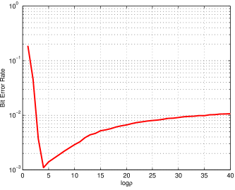
Figure 1: BER vs. $\log\rho$ for a $10\times 10$ uncoded system using 64-QAM, $K=20$ and SNR per bit = 19 dB.

IV-B Complexity versus Performance Gain

We shall determine the effect of complexity on the performance gain of sampling decoding over Babai’s decoding. Following [15], we define the gain in squared decoding radius as

$$G\triangleq\frac{R_{\text{Random}}^{2}}{R_{\text{SIC}}^{2}}.$$

From (11) and (28), we get

$$G=8n/\rho_{0},\quad\rho_{0}>1.$$ (29)

It is worth pointing out that $G$ is independent of whether or which algorithm of lattice reduction is applied, because the term $\min_{1\leq i\leq n}r_{i,i}$ has been canceled out.

By substituting (29) in (27), we have

$$K=\left\lceil\left(8en/G\right)^{G/4}\right\rceil,\quad G<8n.$$ (30)

Equation (30) reveals the tradeoff between $G$ and $K$. Larger $G$ requires larger $K$. For fixed performance gain $G$, randomized lattice decoding has polynomial complexity with respect to $n$. More precisely, each call to Rand_SIC incurs $O(n^{2})$ complexity; for fixed $G$, $K=O(n^{G/4})$. Thus the complexity of randomized lattice decoding is $O(n^{2+G/4})$, excluding pre-processing (lattice reduction and QR decomposition). This is the most interesting case for decoding applications, where practical algorithms are desired. In this case, $\rho_{0}$ is linear with $n$ by (29), thus validating that $g(\rho)$ in (22) is indeed negligible.

Table II shows the computational complexity required to achieve the performance gain from $3$ dB to $12$ dB. It can be seen that a significant gain over SIC can be achieved at polynomial complexity. It is particularly easy to recover the first 3 dB loss of Babai’s decoding, which needs $O(\sqrt{n})$ samples only.

We point out that Table II holds in the asymptotic sense. It should be used with caution for finite $n$, as the estimate of $G$ could be optimistic. The real gain certainly cannot be larger than the gap to ML decoding. The closer Klein’s algorithm performs to ML decoding, the more optimistic the estimate will be. This is because the decoding radius alone does not completely characterize the performance. Nonetheless, the estimate is quite accurate for the first few dBs, as will be shown in simulation results.

TABLE II: Required value of $K$ to achieve gain $G$ in randomized lattice decoding (the complexity excludes pre-processing)

Gain in dB	$G$	$\rho_{0}$	$K$	Complexity
$3$	$2$	$4n$	$\sqrt{4en}$	$O(n^{5/2})$
$6$	$4$	$2n$	$2en$	$O(n^{3})$
$9$	$8$	$n$	$(en)^{2}$	$O(n^{4})$
$12$	$16$	$n/2$	$(en/2)^{4}$	$O(n^{6})$

IV-C Limits

Sampling decoding has its limits. Because equation (29) only holds when $\rho_{0}>1$, we must have $G<8n$. In fact, our analysis requires that $\rho_{0}$ is not close to 1. Therefore, at best sampling decoding can achieve a linear gain $G=O(n)$. To achieve near-ML performance asymptotically, $G$ should exceed the proximity factor, i.e.,

$$F_{\text{SIC}}\leq G=8n/\rho_{0},\quad\rho_{0}>1.$$ (31)

However, this cannot be satisfied asymptotically, since $F_{\text{SIC}}$ is exponential in $n$ for LLL reduction (and is $n^{2}$ for dual KZ reduction). Of note is the proximity factor of random lattice decoding $F_{\text{Random}}=F_{\text{SIC}}/G$, which is still exponential for LLL reduction.

Further, if we do want to achieve $G>8n$, sampling decoding will not be useful. One can still apply Klein’s choice $\rho=n$, but it will be even less efficient than uniform sampling. Therefore, at very high dimensions, sampling decoding might be worse than sphere decoding if one sticks to ML decoding.

The $G=O(n)$ gain is asymptotically vanishing compared to the exponential proximity factor of LLL. Even this $O(n)$ gain is mostly of theoretic interest, since $K$ will be huge. Thus, sampling is probably best suited as a polynomial-complexity algorithm to recover a fixed amount of the gap to ML decoding.

Nonetheless, sampling decoding is quite useful for a significant range of $n$ in practice. On one hand, it is known that the real gap between SIC and ML decoding is smaller than the worst-case bounds; we can run simulations to estimate the gap, which is often less than 10 dB for $n\leq 32$. On the other hand, the estimate of $G$ does not suffer from such worst-case bounds; thus it has good accuracy. For such a range of $n$, sampling decoding performs favorably, as it can achieve near-ML performance at polynomial complexity.

V IMPLEMENTATION

In this Section, we address several issues of implementation. In particular, we propose an efficient implementation of the sampler, extend it to complex-valued lattices, to soft output, and to MMSE.

V-A Efficient Randomized Rounding

The core of Klein’s decoder is the randomized rounding with respect to discrete Gaussian distribution (15). Unfortunately, it can not be generated by simply quantizing the continuous Gaussian distribution. A rejection algorithm is given in [34] to generate a random variable with the discrete Gaussian distribution from the continuous Gaussian distribution; however, it is efficient only when the variance is large. From (15), the variance in our problem is less than $1/\log\rho_{0}$. From the analysis in Section IV, we recognize that $\rho_{0}$ can be large, especially for small $K$. Therefore, the implementation complexity can be high.

Here, we propose an efficient implementation of random rounding by truncating the discrete Gaussian distribution and prove the accuracy of this truncation. Efficient generation of $Q$ results in high decoding speed.

In order to generate the random integer $Q$ with distribution (15), a naive way is to calculate the cumulative distribution function

$$F_{c,r}(q)\triangleq P\left(Q\leq q\right)=\sum_{i\leq q}P\left(Q=i\right).$$ (32)

Obviously, $P(Q=q)=F_{c,r}(q)-F_{c,r}(q-1)$. Therefore, we generate a real-valued random number $z$ that is uniformly distributed on $[0,1]$; then we let $Q=q$ if $F_{c,r}(q-1)\leq z<F_{c,r}(q)$. A problem is that this has to be done online, since $F_{c,r}(q)$ depends on $c$ and $r$. The implementation complexity can be high, which will slow down decoding.

We now try to find a good approximation to distribution (15). Write $r=\lfloor r\rfloor+a$, where $0\leq a<1$. Let $b=1-a$. Distribution (15) can be rewritten as follows

$$P(Q=q)=\left\{\begin{array}[]{l}e^{-c(a+i)^{2}}/s,\quad q=\lfloor r\rfloor-i\\ e^{-c(b+i)^{2}}/s,\quad q=\lfloor r\rfloor+1+i\end{array}\right.$$ (33)

where $i\geq 0$ is an integer and

$$s=\sum_{i\geq 0}(e^{-c\left(a+i\right)^{2}}+e^{-c\left(b+i\right)^{2}}).$$

Because $A=\log\rho/\min_{i}\|\mathbf{\hat{b}}_{i}\|^{2}$, for every invocation of Rand_Round${}_{c}\left(r\right)$, we have $c\geq\log\rho$. We use this bound to estimate the probability $P_{2N}$ that $r$ is rounded to the $2N$-integer set $\left\{\lfloor r\rfloor-N+1\text{,...,}\lfloor r\rfloor\text{,...,}\lfloor r\rfloor+N\right\}$. Now the probability that $q$ is not one of these $2N$ points can be bounded as

$$1-P_{2N} = \sum_{i\geq N}\left(e^{-c(a+i)^{2}}+e^{-c(b+i)^{2}}/s\right)$$ (34)

$$\leq \left(1+\rho^{-(2N+1)}+\rho^{-(4N+4)}\cdots\right)\cdot$$

$$\left(e^{-c(a+N)^{2}}+e^{-c(b+N)^{2}}\right)/s$$

$$< \left(1+O(\rho^{-(2N+1)})\right)\cdot$$

$$\left(e^{-c(a+N)^{2}}+e^{-c(b+N)^{2}}\right)/s.$$

Here, and throughout this subsection, $O(\cdot)$ is with respect to $N$. Since $s\geq e^{-ca^{2}}$ and $s\geq e^{-cb^{2}}$, we have

$$1-P_{2N} < \left(1+O(\rho^{-(2N+1)})\right)\cdot$$ (35)

$$\left(e^{-c(a+N)^{2}}/e^{-ca^{2}}+e^{-c(b+N)^{2}}/e^{-cb^{2}}\right)$$

$$\leq 2\left(1+O(\rho^{-(2N+1)})\right)e^{-N^{2}c}$$

$$= O\left(\rho^{-N^{2}}\right).$$

Hence

$$P_{2N}>1-O(\rho^{-N^{2}}).$$ (36)

Since $\rho>1$, the tail bound (35) decays very fast. Consequently, it is almost sure that a call to Rand_Round${}_{c}\left(r\right)$ returns an integer in $\left\{\lfloor r\rfloor-N+1\text{,...,}\lfloor r\rfloor\text{,...,}\lfloor r\rfloor+N\right\}$ as long as $N$ is not too small. Therefore, we can approximate distribution (15) by $2N$-point discrete distribution as follows.

$$P(Q=q)=\left\{\begin{array}[]{l}e^{-c(a+N-1)^{2}}/s^{\prime}\\ \quad\vdots\\ e^{-ca^{2}}/s^{\prime}\\ e^{-cb^{2}}/s^{\prime}\\ \quad\vdots\\ e^{-c(b+N-1)^{2}}/s^{\prime}\end{array}\right.\begin{array}[]{l}q=\lfloor r\rfloor-N+1\\ \quad\vdots\\ q=\lfloor r\rfloor\\ q=\lfloor r\rfloor+1\\ \quad\vdots\\ q=\lfloor r\rfloor+N\end{array}$$ (37)

where

$$s^{\prime}=\sum_{i=0}^{N-1}(e^{-c(a+i)^{2}}+e^{-c(b+i)^{2}}).$$

Fig. 2 shows the distribution (15), when $r$ $=-5.87$ and $c=3.16$. The values of $r$ and $c$ are the interim results obtained by decoding an uncoded $10\times 10$ system. The distribution of $Q$ concentrates at $\lfloor r\rfloor=-6$ and $\lfloor r\rfloor+1=-5$ with probability 0.9 and 0.08 respectively. Fig. 3 compare the bit error rates associated with different $N$ for an uncoded $10\times 10$ ($n_{T}=n_{R}=10$) system with $K=20$. It is seen that the choice of $N=2$ is indistinguishable from larger $N$. In fact, it is often adequate to choose a 3-point approximation as the probability in the central 3 points is almost one.

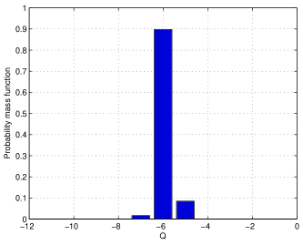
Figure 2: Distribution of $Q$ for $r=-5.87$ and $c=3.16$. $P(Q=-7)=0.02$, $P(Q=-6)=0.9$ and $P(Q=-5)=0.08$.

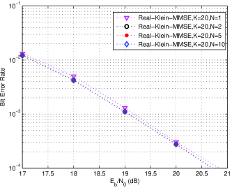
Figure 3: Bit error rate vs. average SNR per bit for a $10\times 10$ uncoded system using 64-QAM.

The following lemma provides a theoretical explanation to the above argument from the viewpoint of statistical distance  [35, Chap. 8]. The statistical distance measures how two probability distributions differ from each other, and is a convenient tool to analyze randomized algorithms. An important property is that applying a deterministic or random function to two distributions does not increase the statistical distance. This implies an algorithm behaves similarly if fed two nearby distributions. More precisely, if the output satisfies a property with probability $p$ when the algorithm uses a distribution $D_{1}$, then the property is still satisfied with probability $\geq p-\Delta(D_{1},D_{2})$ if fed $D_{2}$ instead of $D_{1}$ (see [35, Chap. 8]).

Lemma 3

Let $D$ ($D(i)=P(Q=i)$) be the non-truncated discrete Gaussian distribution, and $D^{\prime}$ be the truncated $2N$-point distribution. Then the statistical distance between $D$ and $D^{\prime}$ satisfies:

$$\Delta(D,D^{\prime})\triangleq\frac{1}{2}\sum_{i\in\mathbb{Z}}|D(i)-D^{\prime}(i)|=O(\rho^{-N^{2}}).$$

Proof:

By definition of $D^{\prime}$, we have:

$$\Delta = \frac{1}{2}\sum_{i<\lfloor r\rfloor-N+1}D(i)+\frac{1}{2}\sum_{i>\lfloor r\rfloor+N}D(i)$$

$$+\frac{1}{2}\left|1-\frac{s}{s^{\prime}}\right|\sum_{i=\lfloor r\rfloor-N+1}^{\lfloor r\rfloor+N}D(i)$$

$$= \frac{1}{2}\sum_{i<\lfloor r\rfloor-N+1}D(i)+\frac{1}{2}\sum_{i>\lfloor r\rfloor+N}D(i)+\frac{|s^{\prime}-s|}{2s}$$

$$\leq \sum_{i<\lfloor r\rfloor-N+1}D(i)+\sum_{i>\lfloor r\rfloor+N}D(i),$$

where $s=\sum_{i\geq 0}(e^{-c(a+i)^{2}}+e^{-c(b+i)^{2}})$ and $s^{\prime}=\sum_{i=0}^{N-1}(e^{-c(a+i)^{2}}+e^{-c(b+i)^{2}})$. The result then derives from (35).    

As a consequence, the statistical distance between the distributions used by Klein’s algorithm corresponding to the non-truncated and truncated Gaussians is $nKO(\rho^{-N^{2}})$. Hence, the behavior of the algorithm with truncated Gaussian is almost the same.

V-B Complex Randomized Lattice Decoding

Since the traditional lattice formulation is only directly applicable to a real-valued channel matrix, sampling decoding was given for the real-valued equivalent of the complex-valued channel matrix. This approach doubles the channel matrix dimension and may lead to higher complexity. From the complex lattice viewpoint [36], we study the complex sampling decoding. The advantage of this algorithm is that it reduces the computational complexity by incorporating complex LLL reduction [36].

Due to the orthogonality of real and imaginary part of the complex subchannel, real and imaginary part of the transmit symbols are decoded in the same step. This allows us to derive complex sampling decoding by performing randomized rounding for the real and imaginary parts of the received vector separately.

In this sense, given the real part of input $\mathbf{y}$, sampling decoding returns real part of $\mathbf{z}$ with probability

$$P\left(\mathfrak{\Re}\left(\mathbf{z}\right)\right)\geq\frac{1}{\prod_{i\leq n}{s(Ar_{i,i}^{2})}}e^{-A\|\mathfrak{\Re}\left(\mathbf{y}\right)-\mathfrak{\Re}\left(\mathbf{z}\right)\|^{2}}.$$ (38)

Similarly, given the imaginary part of input $\mathbf{y}$, sampling lattice decoding returns imaginary part of $\mathbf{z}$ with probability

$$P\left(\mathfrak{\Im}\left(\mathbf{z}\right)\right)\geq\frac{1}{\prod_{i\leq n}{s(Ar_{i,i}^{2})}}e^{-A\|\mathfrak{\Im}\left(\mathbf{y}\right)-\mathfrak{\Im}\left(\mathbf{z}\right)\|^{2}}.$$ (39)

By multiplying these two probabilities, we get a lower bound on the probability that the complex sampling decoding returns $\mathbf{z}$

$$P(\mathbf{z}) = P\left(\mathfrak{\Re}\left(\mathbf{z}\right)\right)\cdot P\left(\mathfrak{\Im}\left(\mathbf{z}\right)\right)$$ (40)

$$\geq \frac{1}{\prod_{i\leq n}{s}^{2}{(Ar_{i,i}^{2})}}e^{-A\left(\|\mathfrak{\Re}\left(\mathbf{y}\right)-\mathfrak{\Re}\left(\mathbf{z}\right)\|^{2}+\|\mathfrak{\Im}\left(\mathbf{y}\right)-\mathfrak{\Im}\left(\mathbf{z}\right)\|^{2}\right)}$$

$$= \frac{1}{\prod_{i\leq n}{s}^{2}{(Ar_{i,i}^{2})}}e^{-A\|\mathbf{y}-\mathbf{z}\|^{2}}.$$

Let $A=\log\rho/\min_{i}r_{i,i}^{2}$, where $\rho>1$. Along the same line of the analysis in the preceding Section, we can easily obtain

$$P(\mathbf{z})>e^{-\frac{4n}{\rho}(1+{g(\rho)})}\cdot\rho^{-\|\mathbf{y}-\mathbf{z}\|^{2}/\min_{1\leq i\leq n}r_{i,i}^{2}}.$$ (41)

Given $K$ calls, inequality (41) implies the choice of the optimum value of $\rho$:

$$K=\left(e\rho_{0}\right)^{4n/\rho_{0}},$$ (42)

and the decoding radius of complex sampling decoding

$$R_{\text{Random}}^{\text{C}}=\sqrt{\frac{4n}{\rho_{0}}}\min_{1\leq i\leq n}r_{i,i}.$$ (43)

Let us compare with the $2n$-dimensional real sampling decoding

$$R_{\text{Random}}^{\text{R }}=\sqrt{\frac{4n}{\rho_{0}}}\min_{1\leq i\leq n}r_{i,i}.$$ (44)

Obviously,

$$R_{\text{Random}}^{\text{C}}=R_{\text{Random}}^{\text{R }}$$ (45)

Real and complex versions of sampling decoding also have the same parameter $A$ for the same $K$.

V-C MMSE-Based Sampling Decoding

The MMSE detector takes the SNR term into account and thereby leading to an improved performance. As shown in [17], MMSE detector is equal to ZF with respect to an extended system model. To this end, we define the $(m+n)\times n$ extended channel matrix $\underline{\mathbf{B}}$ and the $(m+n)\times 1$ extended receive vector $\underline{\mathbf{y}}$ by

$$\underline{\mathbf{B}}=\left[\begin{array}[]{c}\mathbf{B}\\ \sigma\mathbf{I}_{n}\end{array}\right]\text{ \ \ and \ \ }\underline{\mathbf{y}}=\left[\begin{array}[]{c}\mathbf{y}\\ 0_{n,1}\end{array}\right]\text{.}$$

This viewpoint allows us to incorporate the MMSE criterion in the real and complex randomized lattice decoding schemes.

V-D Soft-Output Decoding

Soft output is also available from the samples generated in Rand_SIC. The $K$ candidate vectors $\mathcal{Z=}\left\{\mathbf{z}_{1},\cdots,\mathbf{z}_{K}\right\}$ can be used to approximate the log-likelihood ratio (LLR), as in [37]. For bit $b_{i}\in\{0,1\}$, the approximated LLR is computed as

$$LLR\left(b_{i}\mid\mathbf{y}\right)=\log\frac{\sum_{\mathbf{z}\mathbf{\in}\mathcal{Z}:b_{i}\left(\mathbf{z}\right)=1}\exp\left(-\frac{1}{\sigma^{2}}\|\mathbf{y}-\mathbf{z}\|^{2}\right)}{\sum_{\mathbf{z}\mathbf{\in}\mathcal{Z}:b_{i}\left(\mathbf{z}\right)=0}\exp\left(-\frac{1}{\sigma^{2}}\|\mathbf{y}-\mathbf{z}\|^{2}\right)}$$ (46)

where $b_{i}\left(\mathbf{z}\right)$ is the $i$-th information bit associated with the sample $\mathbf{z}$. The notation $\mathbf{z}:b_{i}\left(\mathbf{z}\right)=\mu$ means the set of all vectors $\mathbf{z}$ for which $b_{i}\left(\mathbf{z}\right)=\mu$.

V-E Other issues

Sampling decoding allows for fully parallel implementation, since the samples can be taken independently from each other. Thus the decoding speed could be as high as that of a standard lattice-reduction-aided decoder if it is implemented in parallel.

For SIC, the effective LLL reduction suffices, which has average complexity $O(n^{3}\log n)$ [38], and the LLL algorithm can output the matrices $\mathbf{Q}$ and $\mathbf{R}$ of the QR decomposition.

Since Klein’s decoding is random, there is a small chance that all the $K$ samples are further than the Babai point. Therefore, it is worthwhile always running Babai’s algorithm in the very beginning. The call can be stopped if the nearest sample point found has distance $\leq\frac{1}{2}\min_{1\leq i\leq n}r_{i,i}$.

VI SIMULATION RESULTS

This section examines the performance of sampling decoding. We assume perfect channel state information at the receiver. For comparison purposes, the performances of Babai’s decoding, lattice reduction aided MMSE-SIC decoding, iterative lattice reduction aided MMSE list decoding [25], and ML decoding are also shown. Monte Carlo simulation was used to estimate the bit error rate with Gray mapping.

For LLL reduction, small values of $\delta$ lead to fast convergence, while large values of $\delta$ lead to a better basis. In our application, increasing $\delta$ will increase the decoding radius $R_{\text{Random}}$. Since lattice reduction is only performed once at the beginning of each block, the complexity of LLL reduction is shared by the block. Thus, we set $\delta$=0.99 for the best performance. The reduction can be speeded up by applying $\delta=0.75$ to obtain a reduced basis, then applying $\delta=0.99$ to further reduce it.

Fig. 4 shows the bit error rate for an uncoded system with $n_{T}=n_{R}=10$, $64$-QAM and LLL reduction ($\delta=0.99$). Observe that even with $15$ samples (corresponding to a theoretic gain $G=3$ dB), the performance of the real Klein’s decoding enhanced by LLL reduction is considerably better (by $2.4$ dB) than that of Babai’s decoding. Compared to iterative lattice reduction aided MMSE list decoding with $25$ samples in [25], the real Klein’s decoding offers not only the improved BER performance (by $1.5$ dB) but also the promise of smaller list size. MMSE-based real Klein’s decoding can achieve further improvement of $1$ dB. We found that $K=25$ (theoretic gain $G=4$ dB) is sufficient for Real MMSE-based Klein’s decoding to obtain near-optimum performance for uncoded systems with $n_{T}=n_{R}\leq 10$; the SNR loss is less than $0.5$ dB. The complex version of MMSE Klein’s decoding exhibits about $0.2$ dB loss at a BER of $10^{-4}$ when compared to the real version. Note that the complex LLL algorithm has half of the complexity of real LLL algorithm. At high dimensions, the real LLL algorithm seems to be slightly better than complex LLL, although their performances are indistinguishable at low dimensions [36].

Fig. 5 shows the frame error rate for a $4\times 4$ MIMO system with $4$-QAM, using a rate-$1/2$, irregular $\left(256,128,3\right)$ low-density parity-check (LDPC) code of codeword length 256 (i.e., 128 information bits). Each codeword spans one channel realization. The parity check matrix is randomly constructed, but cycles of length $4$ are eliminated. The maximum number of decoding iterations is set at 50. It is seen that the soft-output version of sampling decoding is also nearly optimal when $K=24$, with a performance very close to maximum a posterior probability (MAP) decoding.

Fig. 6 and Fig. 7 show the achieved performance of sampling decoding for the $2\times 2$ Golden code [39] using $16$-QAM and $4\times 4$ Perfect code using $64$-QAM [8]. The decoding lattices are of dimension 8 and 32 in the real space, respectively. In Fig. 5, the real MMSE-based Klein decoder with $K=10$ ($G=3$ dB) enjoys 2-dB gain. In Fig. 6, the complex MMSE-based Klein decoder with $K=20$ ($G=3$ dB), $K=71$ ($G=5$ dB) and $K=174$ ($G=6$ dB) enjoys 3-dB, 4-dB and 5-dB gain respectively. It again confirms that the proposed sampling decoding considerably narrows the gap to ML performance. Reference [19] proposed a decoding scheme for the Golden code that suffers a loss of $3$ dB with respect to ML decoding, i.e., the performance is about the same as that of LR-MMSE-SIC. These experimental results are expected, as LLL reduction has been shown to increase the probability of finding the closest lattice point. Also, increasing the list size $K$ available to the decoder improves its performance gain. Varying the number of samples $K$ allows us to negotiate a trade-off between performance and computational complexity.

Fig. 8 compares the average complexity of Babai’s decoding, Klein’s decoding and sphere decoding for uncoded MIMO systems using $64$-QAM. The channel matrix remains constant throughout a block of length $100$ and the pre-processing is only performed once at the beginning of each block. It can be seen that the average flops of Klein’s decoding increases slowly with the dimension, while the average flops of sphere decoding are exponential in dimension. The computational complexity gap between Klein’s decoding and Babai’s decoding is nearly constant for $G=3$ dB or 6 dB. This is because the complexity of Klein’s decoding (excluding pre-processing) is no more than $O(n^{3})$ for $G\leq 6$ dB (cf. Table II), meaning the overall complexity is still $O(n^{3}\log n)$ (including pre-processing), the same order as that of Babai’s decoding.

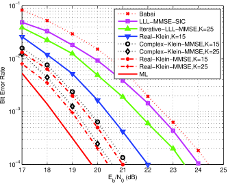
Figure 4: Bit error rate vs. average SNR per bit for the uncoded $10\times 10$ system using 64-QAM.

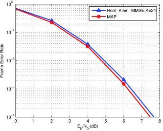
Figure 5: Frame error rate vs. average SNR per bit for the $4\times 4$ rate-1/2 LDPC code of codeword length 256 using 4-QAM.

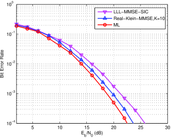
Figure 6: Bit error rate vs. average SNR per bit for the $2\times 2$ Golden code using 16-QAM.

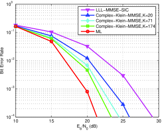
Figure 7: Bit error rate vs. average SNR per bit for the $4\times 4$ perfect code using 64-QAM.

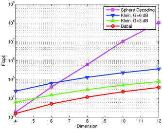
Figure 8: Average number of floating-point operations for uncoded MIMO at average SNR per bit = 17 dB. Dimension $n=2n_{T}=2n_{R}$.

VII CONCLUSIONS

In this paper, we studied sampling-based randomized lattice decoding where the standard rounding in SIC is replaced by random rounding. We refined the analysis of Klein’s algorithm and applied it to uncoded and coded MIMO systems. In essence, Klein’s algorithm is a randomized bounded-distance decoder. Given the number of samples $K$, we derived the optimum parameter $A$ to maximize the decoding radius $R_{\text{Random}}$. Compared to SIC, the best possible gain (measured in squared decoding radius) of our improved decoder is $G=O(n)$. Although it is asymptotically vanishing compared to the exponential factor of LLL reduction, the proposed decoder can well be useful in practice. Of particular interest is that for fixed gain $G$, the value of $K=O(n^{G/4})$ retains the polynomial complexity in $n$. We also proposed an efficient implementation of random rounding which exhibits indistinguishable performance, supported by the statistical distance argument for the truncated discrete Gaussian distribution. The simulations verified that the SNR gain agrees well with $G$ predicted by theory. With the new approach, it is quite practical to recover $6$ dB of the gap to ML decoding, at essentially cubic complexity $O(n^{3})$. The computational structure of the proposed decoding scheme is straightforward and allows for an efficient parallel implementation.

References

- [1] R. Kannan, “Minkowski’s convex body theorem and integer programming,” Math. Oper. Res., vol. 12, pp. 415–440, Aug. 1987.
- [2] G. Hanrot and D. Stehlé, “Improved analysis of Kannan’s shortest vector algorithm,” in Crypto 2007, Santa Barbara, California, USA, Aug. 2007.
- [3] D. Micciancio and P. Voulgaris, “A deterministic single exponential time algorithm for most lattice problems based on Voronoi cell computations,” in STOC’10, Cambridge, MA, USA, Jun. 2010.
- [4] M. O. Damen, H. E. Gamal, and G. Caire, “On maximum likelihood detection and the search for the closest lattice point,” IEEE Trans. Inf. Theory, vol. 49, pp. 2389–2402, Oct. 2003.
- [5] E. Viterbo and J. Boutros, “A universal lattice code decoder for fading channels,” IEEE Trans. Inf. Theory, vol. 45, pp. 1639–1642, Jul. 1999.
- [6] E. Agrell, T. Eriksson, A. Vardy, and K. Zeger, “Closest point search in lattices,” IEEE Trans. Inf. Theory, vol. 48, pp. 2201–2214, Aug. 2002.
- [7] J. Jaldén and B. Ottersen, “On the complexity of sphere decoding in digital communications,” IEEE Trans. Signal Process., vol. 53, pp. 1474–1484, Apr. 2005.
- [8] F. Oggier, G. Rekaya, J.-C. Belfiore, and E. Viterbo, “Perfect space time block codes,” IEEE Trans. Inf. Theory, vol. 52, pp. 3885–3902, Sep. 2006.
- [9] E. Biglieri, Y. Hong, and E. Viterbo, “On fast-decodable space-time block codes,” IEEE Trans. Inf. Theory, vol. 55, pp. 524–530, Feb. 2009.
- [10] L. Babai, “On Lovász’ lattice reduction and the nearest lattice point problem,” Combinatorica, vol. 6, no. 1, pp. 1–13, 1986.
- [11] H. Yao and G. W. Wornell, “Lattice-reduction-aided detectors for MIMO communication systems,” in Proc. Globecom’02, Taipei, China, Nov. 2002, pp. 17–21.
- [12] C. Windpassinger and R. F. H. Fischer, “Low-complexity near-maximum-likelihood detection and precoding for MIMO systems using lattice reduction,” in Proc. IEEE Information Theory Workshop, Paris, France, Mar. 2003, pp. 345–348.
- [13] M. Taherzadeh, A. Mobasher, and A. K. Khandani, “LLL reduction achieves the receive diversity in MIMO decoding,” IEEE Trans. Inf. Theory, vol. 53, pp. 4801–4805, Dec. 2007.
- [14] X. Ma and W. Zhang, “Performance analysis for V-BLAST systems with lattice-reduction aided linear equalization,” IEEE Trans. Commun., vol. 56, pp. 309–318, Feb. 2008.
- [15] C. Ling, “On the proximity factors of lattice reduction-aided decoding,” IEEE Trans. Signal Process., submitted for publication. [Online]. Available: http://www.commsp.ee.ic.ac.uk/ cling/
- [16] J. Jaldén and P. Elia, “LR-aided MMSE lattice decoding is DMT optimal for all approximately universal codes,” in Proc. Int. Symp. Inform. Theory (ISIT’09), Seoul, Korea, 2009.
- [17] D. Wübben, R. Böhnke, V. Kühn, and K. D. Kammeyer, “Near-maximum-likelihood detection of MIMO systems using MMSE-based lattice reduction,” in Proc. IEEE Int. Conf. Commun. (ICC’04), Paris, France, Jun. 2004, pp. 798–802.
- [18] P. Klein, “Finding the closest lattice vector when it’s unusually close,” Proc. ACM-SIAM Symposium on Discrete Algorithms, pp. 937–941, 2000.
- [19] G. R.-B. Othman, L. Luzzi, and J.-C. Belfiore, “Algebraic reduction for the Golden code,” in IEEE Int. Conf. Commun. (ICC’09), Dresden, Germany, Jun. 2009.
- [20] L. Luzzi, G. R.-B. Othman, and J.-C. Belfiore, “Augmented lattice reduction for MIMO decoding,” IEEE Trans. Wireless Commun., vol. 9, pp. 2853–2859, Sep. 2010.
- [21] D. W. Waters and J. R. Barry, “The Chase family of detection algorithms for multiple-input multiple-output channels,” IEEE Trans. Signal Process., vol. 56, pp. 739–747, Feb. 2008.
- [22] C. Windpassinger, L. H.-J. Lampe, and R. F. H. Fischer, “From lattice-reduction-aided detection towards maximum-likelihood detection in MIMO systems,” in Proc. Int. Conf. Wireless and Optical Communications, Banff, Canada, Jul. 2003.
- [23] K. Su and F. R. Kschischang, “Coset-based lattice detection for MIMO systems,” in Proc. Int. Symp. Inform. Theory (ISIT’07), Jun. 2007, pp. 1941–1945.
- [24] J. Choi and H. X. Nguyen, “SIC based detection with list and lattice reduction for MIMO channels,” IEEE Trans. Veh. Technol., vol. 58, pp. 3786–3790, Sep. 2009.
- [25] T. Shimokawa and T. Fujino, “Iterative lattice reduction aided MMSE list detection in MIMO system,” in International Conference on Advanced Technologies for Communications ATC’08, Oct. 2008, pp. 50–54.
- [26] H. Najafi, M. E. D. Jafari, and M. O. Damen, “On the robustness of lattice reduction over correlated fading channels,” 2010, submitted. [Online]. Available: http://www.ece.uwaterloo.ca/ modamen/submitted/Journal_TWC.pdf
- [27] P. Q. Nguyen and T. Vidick, “Sieve algorithms for the shortest vector problem are practical,” J. of Mathematical Cryptology, vol. 2, no. 2, 2008.
- [28] C. Gentry, C. Peikert, and V. Vaikuntanathan, “Trapdoors for hard lattices and new cryptographic constructions,” in 40th Annual ACM Symposium on Theory of Computing, Victoria, Canada, 2008, pp. 197–206.
- [29] P. M. Gruber and C. G. Lekkerkerker, Geometry of Numbers. Amsterdam, Netherlands: Elsevier, 1987.
- [30] J. W. S. Cassels, An Introduction to the Geometry of Numbers. Berlin, Germany: Springer-Verlag, 1971.
- [31] R. A. Horn and C. R. Johnson, Matrix Analysis. Cambridge, UK: Cambridge University Press, 1985.
- [32] A. K. Lenstra, J. H. W. Lenstra, and L. Lovász, “Factoring polynomials with rational coefficients,” Math. Ann., vol. 261, pp. 515–534, 1982.
- [33] P. Q. Nguyen and D. Stehlé, “LLL on the average,” in Proc. ANTS-VII, ser. LNCS 4076. Springer-Verlag, 2006, pp. 238–356.
- [34] L. Devroye, Non-Uniform Random Variate Generation. New York: Springer-Verlag, 1986, pp. 117.
- [35] D. Micciancio and S. Goldwasser, Complexity of Lattice Problems: A Cryptographic Perspective. Boston: Kluwer Academic, 2002.
- [36] Y. H. Gan, C. Ling, and W. H. Mow, “Complex lattice reduction algorithm for low-complexity full-diversity MIMO detection,” IEEE Trans. Signal Process., vol. 57, pp. 2701–2710, Jul. 2009.
- [37] B. M. Hochwald and S. ten Brink, “Achieving near-capacity on a multiple-antenna channel,” IEEE Trans. Commun., vol. 51, pp. 389–399, Mar. 2003.
- [38] C. Ling and N. Howgrave-Graham, “Effective LLL reduction for lattice decoding,” in Proc. Int. Symp. Inform. Theory (ISIT’07), Nice, France, Jun. 2007.
- [39] J.-C. Belfiore, G. Rekaya, and E. Viterbo, “The Golden code: A 2 x 2 full-rate space-time code with nonvanishing determinants,” IEEE Trans. Inf. Theory, vol. 51, pp. 1432–1436, Apr. 2005.