Graviton confinement inside hypermonopoles of any dimension

Abstract

We show the generic existence of metastable massive gravitons in the four-dimensional core of self-gravitating hypermonopoles in any number of infinite-volume extra-dimensions. Confinement is observed for Higgs and gauge bosons couplings of the order unity. Provided these resonances are light enough, they may realise the Dvali–Gabadadze–Porrati mechanism by inducing a four-dimensional gravity law on some intermediate length scales. The effective four-dimensional Planck mass is shown to be proportional to a negative power of the graviton mass. As a result, requiring gravity to be four-dimensional on cosmological length scales may solve the mass hierarchy problem.

1 Introduction

The old and more recent interest in the existence of space-like extra-dimensions has led to three main ways of accommodating their presence with an apparent four-dimensional world [1, 2, 3]. In String Theory, extra-dimensions are compactified and can be probed only at an energy scale exceeding their inverse radius. The non-observation of the associated Kaluza–Klein (KK) excitations at colliders have pushed such a scale above the $\mathrm{TeV}$. However, motivated by orbifold constructions, it has been realised that the typical size of the extra-dimensions probed by gravity could be much larger than the one felt by the gauge (and matter) fields [4, 5, 6]. In this picture, our universe could be a four-dimensional brane on which the Standard Model particles are confined, embedded in a higher-dimensional bulk  [7, 8, 9, 10, 11]. Still, gravity is tested to be four-dimensional on length-scales ranging from the micrometers to the cosmological distances [12, 13]. A micrometer is nevertheless much larger than a $\mathrm{TeV}^{-1}$ while the current cosmic acceleration might be the signature that gravity is actually no longer standard on the largest length scales [14]. These motivations have led to two other gravity confinement mechanisms. In the Randall–Sundrum (RS) models, the extra-dimensions felt by gravity are non-compact but still of finite volume such that deviations from four-dimensional physics appear only at lengths smaller than their curvature radius [15]. In the Dvali–Gabadadze–Porrati (DGP) models, the extra-dimensions are non-compact and of infinite volume. Gravity can be observed as four-dimensional provided the graviton flux between two masses is prevented to leak into the extra-dimensions. In the original DGP model, this is obtained by adding a (quantum induced) four-dimensional Einstein–Hilbert term on the brane [16, 17]. Although it has been argued that some instabilities should show up in the original approach [18, 19], stable extensions have been proposed since [20, 21, 22, 23, 24, 25, 26, 27]. The so-called regularised DGP models assume an ad-hoc varying gravitational coupling constant along the extra-dimensions such that gravitons are reflected back onto the brane in the same way as a varying dielectric constant reflects photons. Assuming the gravity action to be

$$S=\frac{\displaystyle 1}{\displaystyle 2\kappa^{2}}\int{\sqrt{|g|}\,R\,\mathcal{F}(X)\,\mathrm{d}^{n_{\mathrm{e}}+4}X},$$ (1)

where $n_{\mathrm{e}}$ stands for the number of extra-dimension, $R$ is the Ricci scalar and $g$ is the determinant of the metric tensor, it has been shown that $4D$-like gravity can be recovered provided the function $\mathcal{F}(X)$ is peaked enough in a narrow region around the brane [28, 29]. However, the existence of a similar mechanism in a well-defined physical framework is a non-trivial issue. Indeed, the role of the function $\mathcal{F}$ in Eq. (1) could be played by $g(X)$ if there are non-vanishing stress tensor sources in the bulk [30]. A varying Planck mass can also be obtained by considering a dilaton $\psi$ that would condense on the brane such that $\mathcal{F}(X)=\exp[\psi(X)]$ has the required profile. In any case, none of these fields would be independent and their equations of motion have to be solved in a given field theoretical setup to address this question.

This has been done in Refs. [31, 32] in a scalar-tensor theory of gravity by considering our brane to be a self-gravitating topological defect [33, 34, 35, 36, 37]. The core is a flat four-dimensional spacetime supposed to be our universe while the non-trivial defect-forming field configurations curve the extra-dimensions. Such a defect can be formed by the spontaneous breakdown of a local symmetry in the bulk whose stress-tensor ends up being non-vanishing only in a region defining the brane thickness. Typically, it is given by the Compton wavelength of the various defect-forming fields. The extra-dimensional spacetime is asymptotically flat and of infinite volume, as in the DGP model. In six dimensions, this can be obtained by breaking a local $U(1)$ symmetry to form a hyperstring whose core has three spatial dimensions (there is $n_{\mathrm{e}}=2$ extra-dimensions). The seven-dimensional version is a ’t Hooft-Polyakov hypermonopole obtained by breaking an $SO(3)$ symmetry in $n_{\mathrm{e}}=3$ extra-dimensions. As shown in Ref. [31], reflecting gravitons onto the defect core requires a violation of the positivity energy conditions in General Relativity [38]. This happens to be impossible for the hyperstring unless one adds a source of negative energy in the bulk. As a matter of fact, a negative cosmological constant does the job and the model becomes of the RS type, with finite volume extra-dimensions and a severe fine-tuning problem [39, 40]. It is well known that a constant positive curvature term in the Einstein equations behaves like a perfect fluid with a negative equation of state parameter and can therefore mimic matter with negative pressure [41]. Ref. [32] has shown that this mechanism is indeed at work inside the seven-dimensional hypermonopole: assuming isotropy, the positive curvature of the two-dimensional orthoradial extra-dimensions acts as a potential barrier for the propagation of gravitons. These become resonant and massive. The next question is therefore to determine if curving more than two orthoradial extra-dimensions still allows for a similar gravity confinement in higher dimensional spacetimes.

The present article is devoted to this issue. In the following, we show that the DGP-like graviton confinement mechanism by curvature effects is indeed a generic feature of self-gravitating hypermonopoles and occurs in any asymptotically flat spacetime of strictly more than six dimensions. More precisely, in $4+n_{\mathrm{e}}$ dimensions, hypermonopoles can be formed by the spontaneous breakdown of an $SO(n_{\mathrm{e}})$ symmetry to $SO(n_{\mathrm{e}}-1)$. Moreover, in order to allow for a varying Planck mass in the bulk, gravity is supposed to be of the scalar-tensor type, $\psi$ being the dilaton. After having derived and numerically solved the equations of motion in Sec. 2, we show that the extra-dimensions are of infinite volume and asymptotically flat while being strongly positively curved in an intermediate region. Such a configuration is obtained without fine-tuning and naturally occurs for values of the field coupling constant of the order unity. In Sec. 3, we solve for the propagation of spin-two fluctuations along the brane and find strongly peaked massive metastable resonances. We then illustrate how these resonances may realise the DGP mechanism by deriving the resulting Newtonian potential on the brane: it remains $(4+n_{\mathrm{e}})$-dimensional at small and large distances but behaves as $d$-dimensional in an intermediate range with $d<4+n_{\mathrm{e}}$. Finally, we discuss the mass hierarchy problem and show that the four-dimensional effective Newton constant is proportional to a positive power of the mass $m_{\mathrm{g}}$ of the lightest associated graviton resonances. This property is analogous to the existence of a cross-over distance at which gravity becomes $N$-dimensional in the DGP regularised models [28, 29]. In terms of the Planck mass, we find in Eq. (75) that

$$M_{\mathrm{Pl}}^{2}\propto\frac{\displaystyle M^{n_{\mathrm{e}}+2}}{\displaystyle m_{\mathrm{g}}^{n_{\mathrm{e}}}}\,,$$ (2)

where $M$ stands for the $N$-dimensional Planck mass. Since four-dimensional gravity requires extremely light resonances, our mechanism necessarily implies a very small four-dimensional gravity coupling constant. Finally, concerning the smallest length scales, we show that the distance under which gravity is again $N$-dimensional depends on the gravitational redshift induced by the hypermonopole forming fields. It can be made arbitrarily small, independently of the graviton masses, provided the Higgs and gauge bosons have masses close to the Planck mass $M$ in $N$ dimensions.

2 Hypermonopoles of any dimension

In this section, we assume our universe to be the four-dimensional core of a hypermonopole living in $N=4+n_{\mathrm{e}}$ dimensions. This topological defect can be formed by spontaneously breaking an $SO(n_{\mathrm{e}})$ symmetry to $SO(n_{\mathrm{e}}-1)$. We impose this symmetry to be local such that the defect does not exhibit long range interactions and has a localised stress tensor allowing asymptotically flat extra-dimensions. As mentioned in the introduction, gravity is assumed to be of the scalar-tensor type to allow for a varying effective Planck mass along the extra-dimensions. In the Jordan frame, the action describing this system reads

$$S = \frac{\displaystyle 1}{\displaystyle 2\kappa^{2}}\int e^{\psi}\sqrt{|g|}\left[R-g^{AB}\partial_{A}\psi\partial_{B}\psi-U(\psi)\right]\mathrm{d}^{N}x$$ (3)

$$+\int\sqrt{|g|}\left[-\frac{\displaystyle 1}{\displaystyle 2}g^{AB}\mathcal{D}_{A}\boldsymbol{\Phi}\cdot\mathcal{D}_{B}\boldsymbol{\Phi}+\frac{\displaystyle 1}{\displaystyle 8}\mathrm{Tr}\negthinspace\left(\boldsymbol{\mathcal{H}}_{AB}\boldsymbol{\mathcal{H}}^{AB}\right)\right.$$

$$\left.-\frac{\displaystyle\lambda}{\displaystyle 8}\left(\boldsymbol{\Phi}\cdot\boldsymbol{\Phi}-v^{2}\right)^{2}\right]\mathrm{d}^{N}x,$$

where the $SO(n_{\mathrm{e}})$ Higgs field is an $n_{\mathrm{e}}$-dimensional vector $\boldsymbol{\Phi}=\{\phi^{a}\}$ with $a\in\{1,2,\dots,n_{\mathrm{e}}\}$. Gauge invariance under local $SO(n_{\mathrm{e}})$ transformations is ensured by defining the covariant derivatives as

$$\mathcal{D}_{A}\boldsymbol{\Phi}\equiv\partial_{A}\boldsymbol{\Phi}-q\boldsymbol{\mathcal{C}}\negthinspace_{A}\boldsymbol{\Phi},$$ (4)

where $q$ is the Higgs charge and $\boldsymbol{\mathcal{C}}\negthinspace_{A}=\{(C_{A})^{ab}\}$ are the gauge field matrices. The associated field strength tensor matrices are given by

$$\boldsymbol{\mathcal{H}}_{AB}\equiv\partial_{A}\boldsymbol{\mathcal{C}}\negthinspace_{B}-\partial_{B}\boldsymbol{\mathcal{C}}\negthinspace_{A}-q\left[\boldsymbol{\mathcal{C}}\negthinspace_{A},\boldsymbol{\mathcal{C}}\negthinspace_{B}\right].$$ (5)

The last term in Eq. (3) is the Higgs potential $V(\boldsymbol{\Phi})$ and breaks $SO(n_{\mathrm{e}})$ to $SO(n_{\mathrm{e}}-1)$ such that the topology of the vacuum manifold is the same as the $n$-sphere $S^{n}\cong SO(n_{\mathrm{e}})/SO(n_{\mathrm{e}}-1)$, where we have defined

$$n\equiv n_{\mathrm{e}}-1.$$ (6)

Since the $n^{\mathrm{th}}$ homotopy group $\pi_{n}(S^{n})=\mathbb{Z}$ is non-trivial, we expect the formation of hypermonopoles mapping $SO(n_{\mathrm{e}})$ to the $n_{\mathrm{e}}$ extra-dimensions [42]. In Eq. (3), the quantity $U(\psi)$ encodes the dilaton potential in the Jordan frame. For simplicity, we choose the dilaton to be a free massive particle of mass $m_{\mathrm{d}}$ in the Einstein frame such that

$$U(\psi)=m_{\mathrm{d}}^{2}e^{2\psi/(n+3)}\,.$$ (7)

One can check that the above equations reduce to the hyperstring of Ref. [31] for $n_{\mathrm{e}}=2$ and to the ’t Hooft–Polyakov hypermonopole of Ref. [32] when $n_{\mathrm{e}}=3$.

In the following, after having introduced our Ansatz for the field profiles, we derive and solve the equations of motion assuming isotropic extra-dimensions.

2.1 Equations of motion

2.1.1 Gravity sector

Varying the action with respect to the metric tensor and the dilaton gives the Einstein–Jordan equations

$$G_{AB} = \mathrm{e}^{-\psi}\kappa^{2}T_{AB}+2\partial_{A}\psi\partial_{B}\psi-\frac{\displaystyle 1}{\displaystyle 2}g_{AB}\left[3\partial_{X}\psi\partial^{X}\psi\right.$$ (8)

$$\left.+U(\psi)\right]+\nabla_{A}\partial_{B}\psi-g_{AB}\Box\psi,$$

$$\Box\psi = \frac{\displaystyle 1}{\displaystyle 2}U(\psi)+\frac{\displaystyle 1}{\displaystyle 2}\frac{\displaystyle\mathrm{d}U}{\displaystyle\mathrm{d}\psi}-\frac{\displaystyle 1}{\displaystyle 2}R-\frac{\displaystyle 1}{\displaystyle 2}\partial_{X}\phi\partial^{X}\psi,$$ (9)

where $\Box\equiv\nabla_{X}\partial^{X}$, $G_{AB}$ is the $N$-dimensional Einstein tensor and $T_{AB}$ the matter stress tensor

$$T_{AB}=\mathcal{D}_{A}\boldsymbol{\Phi}\cdot\mathcal{D}_{B}\boldsymbol{\Phi}-\frac{\displaystyle 1}{\displaystyle 2}g^{CD}\mathrm{Tr}\negthinspace\left(\boldsymbol{\mathcal{H}}_{AC}\boldsymbol{\mathcal{H}}_{BD}\right)+g_{AB}\mathcal{L}_{\mathrm{m}},$$ (10)

where $\mathcal{L}_{\mathrm{m}}$ is the Higgs and gauge field Lagrangian.

2.1.2 Matter sector

The variations of Eq. (3) with respect to the Higgs and gauge fields gives the Klein–Gordon and Maxwell-like equations:

$$\Box\boldsymbol{\Phi}-q\,g^{AB}\left[\left(\nabla_{A}\boldsymbol{\mathcal{C}}\negthinspace_{B}\boldsymbol{\Phi}\right)+\boldsymbol{\mathcal{C}}\negthinspace_{B}\mathcal{D}_{A}\boldsymbol{\Phi}\right]-\frac{\displaystyle\partial V}{\displaystyle\partial\boldsymbol{\Phi}}=0,$$ (11)

and

$$\left(\nabla_{A}\boldsymbol{\mathcal{H}}^{AB}\right)^{ab} + q\,g^{AB}\left[\left(\mathcal{D}_{A}\boldsymbol{\Phi}\right)^{a}\phi^{b}-\left(\mathcal{D}_{A}\boldsymbol{\Phi}\right)^{b}\phi^{a}\right]$$ (12)

$$+ q\left(\boldsymbol{\mathcal{H}}^{AB}\cdot\boldsymbol{\mathcal{C}}\negthinspace_{A}-\boldsymbol{\mathcal{C}}\negthinspace_{A}\cdot\boldsymbol{\mathcal{H}}^{AB}\right)^{ab}=0.$$ (13)

2.1.3 Metric and field Ansatz

Respecting the hyperspherical static symmetry in the $n_{\mathrm{e}}$ extra-dimensions and Poincaré invariance along the brane gives the metric

$$\mathrm{d}s^{2}=g_{AB}\mathrm{d}x^{A}\mathrm{d}x^{B}=e^{\sigma(r)}\eta_{\mu\nu}\mathrm{d}x^{\mu}\mathrm{d}x^{\nu}+\mathrm{d}r^{2}+\omega^{2}(r)\mathrm{d}\Omega_{n}^{2}.$$ (14)

The metric element over $S^{n}$ being

$$\mathrm{d}\Omega_{n}^{2}=\sum_{i=1}^{n}\Upsilon_{i}(\theta_{j<i})\mathrm{d}\theta_{i}^{2},$$ (15)

with $\Upsilon_{1}=1$, $\Upsilon_{2}=\sin^{2}(\theta_{1})$ and

$$\Upsilon_{i}(\theta_{j<i})\equiv\Upsilon_{2}(\theta_{1})\prod_{j=2}^{i-1}\sin^{2}(\theta_{j})\quad\mathrm{for~{}~{}}i=3,\ldots,n~{}.$$ (16)

For a defect configuration, the Higgs field vanishes in the core whereas it asymptotically recovers its vacuum expectation value. Enforcing the spacetime symmetries, we assume a radial field such that

$$\phi^{a}=\varphi(r)\frac{\displaystyle x^{a}}{\displaystyle r}\,,$$ (17)

with $\varphi(0)=0$ and $\varphi(r)\rightarrow v$ when $r\rightarrow\infty$. In Eq. (17), $r^{2}=\delta_{ab}x^{a}x^{b}$ where the $\{x^{a}\}$ stands for the $n_{\mathrm{e}}$ Cartesian coordinates defined by

$$x^{1} = r\cos\theta_{1},\quad x^{2}=r\sin\theta_{1}\cos\theta_{2},$$

$$\vdots$$

$$x^{n} = r\sin\theta_{1}\sin\theta_{2}\dots\sin\theta_{n-1}\cos\theta_{n},$$

$$x^{n_{\mathrm{e}}} = r\sin\theta_{1}\sin\theta_{2}\dots\sin\theta_{n-1}\sin\theta_{n}.$$ (19)

We also assume that the dilaton depends only on the radial coordinate

$$\psi=\psi(r)~{}.$$ (20)

Our Ansatz for the gauge field is the generalisation of the ’t Hooft–Polyakov configuration [43, 44], with a unity winding number. Requiring the stress tensor to vanish at infinity imposes the covariant derivative to vanish. From Eqs. (4) and (17), one gets

$$(C_{\theta_{i}})^{ab}=\frac{\displaystyle 1-Q(r)}{\displaystyle qr^{2}}\left(\frac{\displaystyle\partial x^{a}}{\displaystyle\partial\theta_{i}}x^{b}-\frac{\displaystyle\partial x^{b}}{\displaystyle\partial\theta_{i}}x^{a}\right),$$ (21)

where the dimensionless function $Q(0)=1$ for regularity in the core and $Q(r)\rightarrow 0$ at infinity. All the other $\boldsymbol{\mathcal{C}}\negthinspace_{A}$ are vanishing. Under such an Ansatz, observing that

$$\mathrm{Tr}\negthinspace\left(\boldsymbol{\mathcal{C}}\negthinspace_{\theta_{i}}\boldsymbol{\mathcal{C}}\negthinspace_{\theta_{j}}\right)=-2\left[\frac{\displaystyle 1-Q(r)}{\displaystyle q\omega(r)}\right]^{2}g_{\theta_{i}\theta_{j}},$$ (22)

the gravity and matter sector equations considerably simplify and we write down only the final result in the next section (see the appendix for some intermediate steps).

2.1.4 Dimensionless equations

For convenience, we introduce the following dimensionless quantities. The radial distance can be expressed in unit of the Higgs Compton wavelength such that

$$\rho\equiv m_{\mathrm{h}}r=\sqrt{\lambda}v\,r,$$ (23)

where $m_{\mathrm{h}}$ is the mass of the Higgs boson. Similarly, the dimensionless angular metric coefficient and Higgs field are defined by

$$\varpi\equiv m_{\mathrm{h}}\omega,\qquad f\equiv\frac{\displaystyle\varphi}{\displaystyle v}\,.$$ (24)

The gravity, Higgs and gauge coupling constants account for three dimensionless parameters in the equations of motion (8) to (12) which can be recast as

$$\alpha\equiv\kappa^{2}v^{2},\qquad\epsilon\equiv\frac{\displaystyle q^{2}v^{2}}{\displaystyle\lambda v^{2}}=\frac{\displaystyle m_{\mathrm{b}}^{2}}{\displaystyle m_{\mathrm{h}}^{2}},\qquad\beta\equiv\frac{\displaystyle m_{\mathrm{d}}^{2}}{\displaystyle\lambda v^{2}}=\frac{\displaystyle m_{\mathrm{d}}^{2}}{\displaystyle m_{\mathrm{h}}^{2}}\,,$$ (25)

$m_{\mathrm{b}}$ being the mass of the gauge bosons. After some rather long algebra, a dot denoting differentiation with respect to $\rho$, the dimensionless equations of motion in the gravity sector read

$$\frac{\displaystyle 3}{\displaystyle 2}\ddot{\sigma} + \frac{\displaystyle 3}{\displaystyle 2}\dot{\sigma}^{2}+n\frac{\displaystyle\ddot{\varpi}}{\displaystyle\varpi}+n(n-1)\frac{\displaystyle\dot{\varpi}^{2}-1}{\displaystyle 2\varpi^{2}}+\frac{\displaystyle 3}{\displaystyle 2}n\dot{\sigma}\frac{\displaystyle\dot{\varpi}}{\displaystyle\varpi}$$ (26)

$$= -\alpha e^{\-\psi}\mathcal{E}-\ddot{\psi}-\frac{\displaystyle 3}{\displaystyle 2}\dot{\psi}^{2}-\left(\frac{\displaystyle 3}{\displaystyle 2}\dot{\sigma}+n\frac{\displaystyle\dot{\varpi}}{\displaystyle\varpi}\right)\dot{\psi}-\frac{\displaystyle\bar{U}}{\displaystyle 2}\,,$$

$$\frac{\displaystyle 3}{\displaystyle 2}\dot{\sigma}^{2} + n(n-1)\frac{\displaystyle\dot{\varpi}^{2}-1}{\displaystyle 2\varpi^{2}}+2n\dot{\sigma}\frac{\displaystyle\dot{\varpi}}{\displaystyle\varpi}$$ (27)

$$= \alpha e^{-\psi}\mathcal{P}+\frac{\displaystyle 1}{\displaystyle 2}\dot{\psi}^{2}-\left(2\dot{\sigma}+n\frac{\displaystyle\dot{\varpi}}{\displaystyle\varpi}\right)\dot{\psi}-\frac{\displaystyle\bar{U}}{\displaystyle 2}\,,$$

$$2\ddot{\sigma} + \frac{\displaystyle 5}{\displaystyle 2}\dot{\sigma}^{2}+(n-1)\frac{\displaystyle\ddot{\varpi}}{\displaystyle\varpi}+(n-1)(n-2)\frac{\displaystyle\dot{\varpi}^{2}-1}{\displaystyle 2\varpi^{2}}+2(n-1)\dot{\sigma}\frac{\displaystyle\dot{\varpi}}{\displaystyle\varpi}$$ (28)

$$= -\alpha e^{-\psi}\mathcal{E}_{\perp}-\ddot{\psi}-\frac{\displaystyle 3}{\displaystyle 2}\dot{\psi}^{2}-\left[2\dot{\sigma}+(n-1)\frac{\displaystyle\dot{\varpi}}{\displaystyle\varpi}\right]\dot{\psi}-\frac{\displaystyle\bar{U}}{\displaystyle 2}\,,$$

$$\ddot{\psi} + \frac{\displaystyle 1}{\displaystyle 2}\dot{\psi}^{2}+\left(2\dot{\sigma}+n\frac{\displaystyle\dot{\varpi}}{\displaystyle\varpi}\right)\dot{\psi}=\frac{\displaystyle 1}{\displaystyle 2}\left(\bar{U}+\frac{\displaystyle\mathrm{d}\bar{U}}{\displaystyle\mathrm{d}\psi}-\bar{R}\right).$$ (29)

The dimensionless dilaton potential is $\bar{U}=U/m_{\mathrm{h}}^{2}$ and the dimensionless Ricci scalar $\bar{R}=R/m_{\mathrm{h}}^{2}$ stands for

$$\bar{R}=-4\ddot{\sigma}-5\dot{\sigma}^{2}-2n\frac{\displaystyle\ddot{\varpi}}{\displaystyle\varpi}-n(n-1)\frac{\displaystyle\dot{\varpi}^{2}-1}{\displaystyle\varpi^{2}}-4n\dot{\sigma}\frac{\displaystyle\dot{\varpi}}{\displaystyle\varpi}\,.$$ (30)

The quantities $\mathcal{E}$ and $\mathcal{P}$ are respectively the energy density and pressure generated by the Higgs and gauge fields along the radial extra-dimension 

$$\mathcal{E} = \frac{\displaystyle\dot{f}^{2}}{\displaystyle 2}+\frac{\displaystyle n\dot{Q}^{2}}{\displaystyle 2\epsilon\varpi^{2}}+\frac{\displaystyle n}{\displaystyle 2\varpi^{2}}f^{2}Q^{2}+\frac{\displaystyle n(n-1)}{\displaystyle 4\epsilon\varpi^{4}}(1-Q^{2})^{2}+\bar{V},$$ (31)

$$\mathcal{P} = \frac{\displaystyle\dot{f}^{2}}{\displaystyle 2}+\frac{\displaystyle n\dot{Q}^{2}}{\displaystyle 2\epsilon\varpi^{2}}-\frac{\displaystyle n}{\displaystyle 2\varpi^{2}}f^{2}Q^{2}-\frac{\displaystyle n(n-1)}{\displaystyle 4\epsilon\varpi^{4}}(1-Q^{2})^{2}-\bar{V},$$ (32)

where $\bar{V}(f)$ stands for the dimensionless Higgs potential

$$\bar{V}(f)\equiv\frac{\displaystyle 1}{\displaystyle 8}\left(1-f^{2}\right)^{2}.$$ (33)

The quantity $\mathcal{E}_{\perp}$ appearing in Eq. (28) is the energy density along the orthoradial directions and reads

$$\mathcal{E}_{\perp}=\frac{\displaystyle\dot{f}^{2}}{\displaystyle 2}+\frac{\displaystyle(n-2)\dot{Q}^{2}}{\displaystyle 2\epsilon\varpi^{2}}+\frac{\displaystyle n-2}{\displaystyle 2\varpi^{2}}f^{2}Q^{2}+\frac{\displaystyle(n-1)(n-4)}{\displaystyle 4\epsilon\varpi^{4}}(1-Q^{2})^{2}+\bar{V}.$$ (34)

The dynamical equations for $f$ and $Q$ stem from Eqs. (11) and (12)

$$\ddot{f} + \left(2\dot{\sigma}+n\frac{\displaystyle\dot{\varpi}}{\displaystyle\varpi}\right)\dot{f}-n\frac{\displaystyle fQ^{2}}{\displaystyle\varpi^{2}}-\frac{\displaystyle\mathrm{d}\bar{V}}{\displaystyle\mathrm{d}f}=0,$$ (35)

$$\ddot{Q} + \left[2\dot{\sigma}+(n-2)\frac{\displaystyle\dot{\varpi}}{\displaystyle\varpi}\right]\dot{Q}+\frac{\displaystyle n-1}{\displaystyle\varpi^{2}}(Q-Q^{3})-\epsilon f^{2}Q=0.$$ (36)

These equations match with those of the six-dimensional hyperstring and seven-dimensional hypermonopole derived in Refs. [31, 32]. Let us however notice the presence of new terms for $n>2$ in the orthoradial equation (28) as well as in the associated stress energy in Eq. (34). It is also worth remarking from Eq. (34) that for $n=2$ or $3$, the gauge field is generating a negative potential in the orthoradial extra-dimensions, which becomes again positive for $n>4$.

2.2 Background fields and geometry

2.2.1 Boundary conditions

The boundary conditions for the metric coefficients and fields are fixed by requiring regularity in the core and a Dirac hypermonopole configuration asymptotically. As already discussed, we look for asymptotically flat spacetime, i.e.

$$\lim_{\rho\rightarrow\infty}f(\rho) =1,\qquad\lim_{\rho\rightarrow\infty}Q(\rho)=0,$$

$$\lim_{\rho\rightarrow\infty}\sigma(\rho) =0,\qquad\lim_{\rho\rightarrow\infty}\frac{\displaystyle\varpi(\rho)}{\displaystyle\rho}=1,\qquad\lim_{\rho\rightarrow\infty}\psi(\rho)=0.$$ (37)

Notice that $\sigma$ could be shifted by a constant value since all the equations of motion depend only on $\dot{\sigma}$: this reflects the expected invariance with respect to a rescaling of the internal brane coordinates $x^{\mu}$. We have also chosen the dilaton to vanish at infinity since this minimises its potential energy and $\psi=0$ is an exact solution of Eq. (29) for $\bar{R}=0$. One can check that this last condition is indeed asymptotically fulfilled with the limits of Eq. (2.2.1). Let us notice that the metric far from the core is not a generalisation of the conical flat metric existing around a cosmic string. As can be checked in Eq. (30), as soon as $n(n-1)\neq 0$ one has $\varpi=\rho$, i.e. there is no missing angle (for $\dot{\sigma}=0$).

In the hypermonopole core, the $SO(n_{\mathrm{e}})$ symmetry should be restored and the spacetime geometry has to be regular. As a result, the fields satisfy

$$\lim_{\rho\rightarrow 0}f(\rho) =0,\qquad\lim_{\rho\rightarrow 0}Q(\rho)=1,$$

$$\lim_{\rho\rightarrow 0}\dot{\sigma}(\rho) =0,\qquad\lim_{\rho\rightarrow 0}\frac{\displaystyle\varpi(\rho)}{\displaystyle\rho}=1,\qquad\lim_{\rho\rightarrow 0}\dot{\psi}(\rho)=0.$$ (38)

2.2.2 Solutions

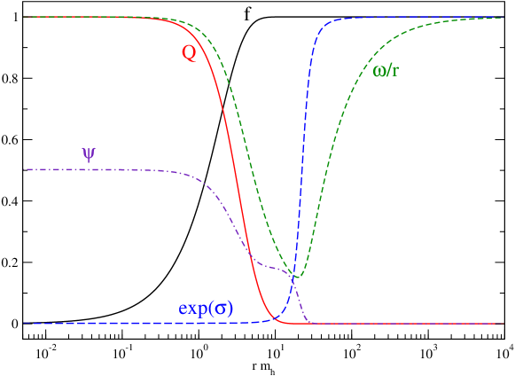
Figure 1: Field and metric profiles forming an eight-dimensional ($n=3$) hypermonopole for $\alpha=2.60$, $\epsilon=0.25$ and $\beta=1.00$ (top). The space-time is flat in the core and at infinity but strongly curved in the intermediate region. The dilaton condenses in the core and traces the energy density distribution. See also Fig. 2.

From Eqs. (2.2.1) and (2.2.1), we have ten boundary conditions to solve the ten-dimensional first order non-linear differential system that can be obtained from the second order Eqs. (26), (28), (29), (35) and (36). Notice that Eq. (27) is not included since this is a constraint equation and is redundant with the previous set, up to a constant which is fixed once the boundary conditions are specified. Finding numerical solutions of this system is non-trivial and we have used the conditioning mesh methods implemented in Ref. [45]. We have first checked our numerical implementation by recovering the $n=1$ and $n=2$ solutions of Refs. [31, 32] before solving the system for $n>2$. Despite the new terms appearing in the equations of motion, we have found hypermonopole solutions for any tested value of $n$. All of them exhibit similar patterns than those found in seven-dimensions. For coupling constant of order unity, the spacetime is strongly curved in an intermediate region where the field derivatives are non-vanishing, and in particular $\varpi$ remains almost stationary with respect to $\rho$. As a result, the hypersurface of the $n$-sphere of radius $\rho$ becomes constant and the extra-dimensions are cylindrically shaped. At further distances, $\varpi\sim\rho$ again and the spacetime becomes flat.

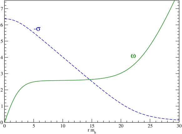
Figure 2: $S^{n}$ hypersurface in the strongly curved region: $\omega(r)$ remains almost constant and the extra-dimensions becomes cylindrically shaped. The gravitational redshift in the core is given by $e^{\sigma(0)}$. The parameters are the same as in Fig. 1.

In Fig. 1, we have represented the field profiles obtained for $n=3$, i.e. in eight spacetime dimensions. The dilaton condenses in the core as a scalar gravity field which passively follows the stress energy distribution. The metric factor $\sigma$ traces the gravitational redshift between the core and the asymptotic spacetime and has been represented with $\omega(r)$ in Fig. 2. Finally, the Higgs and gauge fields are typical of a topological defect configuration. By choosing $\epsilon=0.25$, the gauge bosons are twice lighter than the Higgs boson and condense within a larger extra-dimensional radius. The shift in the condensation radius of the Higgs and gauge field produces the step observed in the dilaton profile (see Fig. 1).

2.2.3 Dependence in the number of dimensions

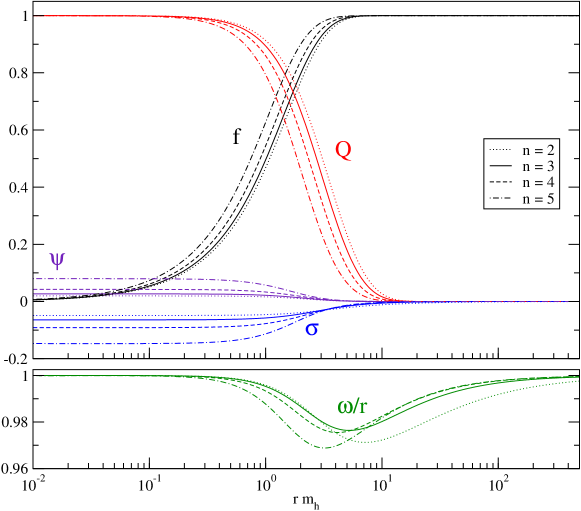
Figure 3: Hypermonopole-forming field profiles in seven ($n=2$) to ten ($n=5$) dimensions. The coupling constants have been fixed to fiducial values $\alpha=0.1$, $\epsilon=0.2$ and $\beta=1$. Gravitational effects are enhanced by increasing $n$ with the exception of the metric coefficient $\omega(r)$. As can be checked in the lower panel, and in Eq. (34), deviations from flat space are first reduced by increasing $n$ from $2$ to $3$, and then amplified for $n>3$.

As discussed in the beginning of this section, the hypermonopole-forming fields exhibit a similar behaviour for all values of $n$. In fact, this can be understood from the equations of motion (26) to (36). The number of dimensions enters these equations through $n$ at two levels.

First, it changes the coupling between the metric coefficients $\varpi$ and $\sigma$, as well as $\varpi$ and the other fields. For a given $\varpi(r)$ profile, one expects all the fields to be more sensitive to it when $n$ becomes large. Let us emphasise that this effect is purely geometrical since it persists when $\alpha\rightarrow 0$. In Fig. 3, we have represented the hypermonopole solutions obtained for an assumed generic set of parameters $\alpha=0.1$, $\epsilon=0.2$, $\beta=1$ and in various dimensions ranging from seven ($n=2$) to ten ($n=5$). The upper panel of this figure illustrates the above-mentioned effect. For larger values of $n$, the gravitational redshift $\sigma(0)$ increases while the dilaton $\psi$, the gauge field $Q$ and the Higgs field $f$ condense in regions closer to the hypermonopole core.

In the equations of motion, $n$ also affects the stress energy tensor produced by the Higgs and gauge fields. As earlier mentioned, the quantity $\mathcal{E}_{\perp}$ in Eq. (34) has a dependence in $(n-1)(n-4)$ which implies the same negative contribution in seven ($n=2$) and eight-dimensions ($n=3$). However, the kinetic terms are multiplied by a factor $(n-2)$ and vanish in seven dimensions. The overall orthoradial energy has therefore a non-trivial dependence in the number of dimension for $n\leq 3$, but should become monotonic for $n>3$. We can verify in the lower panel of Fig. 3 that deviations from flat space in the metric coefficient $\omega(r)$ are first reduced when $n$ goes from $2$ to $3$ before increasing again for $n>3$.

In conclusion, we have found hypermonopole solutions for all tested values of $n$. All the solutions exhibit the typical condensation of Higgs and gauge fields encountered in topological defect configurations. Since the dilaton also condenses, we do have an effective varying Planck mass between the brane and the bulk. There is also a strong gravitational redshift traced by the extra-dimensional profile of $\sigma(r)$. Finally, at the matter field condensation radius, the metric coefficient $\omega(r)$ remains almost constant and the extra-dimensions become cylindrically shaped. In the next section, we solve for the propagation of spin two fluctuations inside such a background and show that gravitons becomes resonant on the length scales at which the extra-dimensions are strongly curved.

3 Resonant gravitons

Restricting our attention to transverse and traceless four-dimensional tensor fluctuations $h_{\mu\nu}$, the metric assumes the form given in Eq. (14) with the replacement $\eta_{\mu\nu}\rightarrow\eta_{\mu\nu}+h_{\mu\nu}$. Their linearised equation of motion can be obtained by expanding the action in Eq. (3) at second order and has already been derived in Ref. [31]. Defining the conformal radial distance $z(r)$ and the rescaled tensor fluctuations $\xi_{\mu\nu}$ by

$$z\equiv m_{\mathrm{h}}\int_{0}^{r}e^{-\sigma(u)/2}\mathrm{d}u,\qquad\xi_{\mu\nu}\equiv e^{3\sigma/4+\psi/2}\varpi^{n/2}h_{\mu\nu},$$ (39)

the equation of motion for the gravitons reads [31]

$$-\xi^{\prime\prime}_{\mu\nu}+\left(W^{2}+W^{\prime}-\frac{\displaystyle e^{\sigma}}{\displaystyle\varpi^{2}}\Delta_{n}-\bar{\Box}_{4}\right)\xi_{\mu\nu}=0,$$ (40)

where a prime stands for derivative with respect to $z$. The quantity $W(z)$ is a superpotential given by

$$W(z)\equiv\frac{\displaystyle 3}{\displaystyle 4}\sigma^{\prime}+\frac{\displaystyle n}{\displaystyle 2}\frac{\displaystyle\varpi^{\prime}}{\displaystyle\varpi}+\frac{\displaystyle 1}{\displaystyle 2}\psi^{\prime},$$ (41)

while $\Delta_{n}$ is the Laplace-Beltrami operator on the $n$-sphere $S^{n}$

$$\Delta_{n}\equiv\sum_{i=1}^{n}\frac{\displaystyle 1}{\displaystyle\Upsilon_{i}}\left(\frac{\displaystyle\partial^{2}}{\displaystyle\partial\theta_{i}^{2}}+\frac{\displaystyle n-i}{\displaystyle\tan\theta_{i}}\frac{\displaystyle\partial}{\displaystyle\partial\theta_{i}}\right),$$ (42)

and $\bar{\Box}_{4}$ is the four-dimensional d’Alembertian

$$\bar{\Box}_{4}\equiv\frac{\displaystyle 1}{\displaystyle m_{\mathrm{h}}^{2}}\eta_{\mu\nu}\partial_{\mu}\partial_{\nu}\,.$$ (43)

In order to solve Eq. (40), it is convenient to perform a four-dimensional Fourier transform and a decomposition over the hyperspherical harmonics ${f_{\ell}^{\boldsymbol{m}}}$ such that the mode functions $u_{M,\ell}(z)$ satisfy

$$-u_{M,\ell}^{\prime\prime}+\left[W^{2}+W^{\prime}+\ell\left(\ell+n-1\right)\frac{\displaystyle e^{\sigma}}{\displaystyle\varpi^{2}}-M^{2}\right]u_{M,\ell}=0.$$ (44)

Here $M^{2}$ and $-\ell(\ell+n-1)$ are the respective eigenvalues of the d’Alembertian and Laplace–Beltrami operator (in Higgs mass unit). This equation assumes the form of a Schrödinger equation of a supersymmetric quantum mechanical system [46]. The central potentials associated with fermionic- and bosonic-like excitations are given by

$$V_{2}(z)=W^{2}+W^{\prime},\qquad V_{1}(z)=W^{2}-W^{\prime}.$$ (45)

Omitting the tensor indices, the ground state $\xi_{0}$ of Eq. (44) is the solution obtained for $M^{2}=\ell=0$ and satisfies

$$\left(\frac{\displaystyle\mathrm{d}}{\displaystyle\mathrm{d}z}+W\right)\left(-\frac{\displaystyle\mathrm{d}}{\displaystyle\mathrm{d}z}+W\right)\xi_{0}=0,$$ (46)

i.e.

$$\xi_{0}\propto\varpi^{n/2}e^{3\sigma/4+\psi/2}.$$ (47)

This zero mode is not normalisable asymptotically. The ground state of the superpartner potential $V_{1}$ is similarly obtained by swapping both terms in Eq. (46) and is given by $\tilde{\xi}_{0}\propto 1/\xi_{0}$. This time, it is not normalisable in the hypermonopole core for $z\rightarrow 0$. As a result, there are no massless gravitons trapped on the brane and “supersymmetry” is broken by the solutions we are interested in (the spectrum associated with $V_{2}$ and $V_{1}$ do not match). Notice that the supersymmetric properties of Eq. (44) ensures that the spectrum is positive and no tachyonic propagation modes can be present.

In order to solve Eq. (40) in general, we assume that the mode functions $u_{M,\ell}$ are normalised such that

$$\int_{0}^{\infty}u_{M,\ell}^{*}(z_{1})u_{M,\ell}^{\phantom{*}}(z_{2})\mathrm{d}M=\delta(z_{1}-z_{2}).$$ (48)

It is now straightforward to check that the Green function for $\xi_{\mu\nu}$ reads

$$G_{\xi}\negthinspace\left(X_{1};X_{2}\right) = -\int\frac{\displaystyle\mathrm{d}^{4}p}{\displaystyle(2\pi)^{4}}e^{ip_{\mu}(x_{1}^{\mu}-x_{2}^{\mu})}$$ (49)

$$\times \sum_{\ell,\boldsymbol{m}}{f_{\ell}^{\boldsymbol{m}}}(\boldsymbol{\theta_{1}}){f_{\ell}^{\boldsymbol{m}}}^{*}(\boldsymbol{\theta_{2}})\int\frac{\displaystyle u_{M,\ell}^{\phantom{*}}(z_{1})u_{M,\ell}^{*}(z_{2})}{\displaystyle M^{2}+\vec{p}^{2}-(p^{0}+i\varepsilon)^{2}}\mathrm{d}M\,.$$

Capital letters have been used for $N$-dimensional coordinates, bold characters for the $n$-dimensional vectors lying on $S^{n}$, and arrows for the usual three-dimensional vectors on the brane. Let us mention that we will not need to specify an explicit expression for the ${f_{\ell}^{\boldsymbol{m}}}$ functions and solely assume they form an orthonormal basis such that

$$\int\left|{f_{\ell}^{\boldsymbol{m}}}(\boldsymbol{\theta})\right|^{2}\mathcal{J}_{n}(\boldsymbol{\theta})\,\mathrm{d}\theta_{1}\mathrm{d}\theta_{2}\dots\mathrm{d}\theta_{n}=1,$$

$$\sum_{\ell,\boldsymbol{m}}{f_{\ell}^{\boldsymbol{m}}}(\boldsymbol{\theta_{1}}){f_{\ell}^{\boldsymbol{m}}}^{*}(\boldsymbol{\theta_{2}})=[\mathcal{J}_{n}(\boldsymbol{\theta_{1}})]^{-1}\,\delta^{n}(\boldsymbol{\theta_{1}}-\boldsymbol{\theta_{2}}),$$ (50)

where $\mathcal{J}_{n}(\boldsymbol{\theta})\mathrm{d}\theta_{1}\cdots\mathrm{d}\theta_{n}$ is the infinitesimal surface element on the unit $n$-sphere so that

$$\mathcal{J}_{n}=\sin^{n-1}(\theta_{1})\sin^{n-2}(\theta_{2})\dots\sin(\theta_{n-1}).$$ (51)

From the Green function, we can derive $h_{\mu\nu}$ for any additional stress energy tensor on the brane. Considering an additional transverse and traceless four-dimensional source $s_{\mu\nu}(x)$ inducing a $N$-dimensional linear stress-tensor perturbation of the form (in Higgs mass unit)

$$\delta T_{\mu\nu}(X)=\lim_{z\rightarrow 0}\frac{\displaystyle\delta(z)}{\displaystyle z^{n}}[\mathcal{J}_{n}(\boldsymbol{\theta})]^{-1}\delta^{n}(\boldsymbol{\theta})s_{\mu\nu}(x),$$ (52)

the tensor fluctuations at $X=X_{1}$ are given by Eq. (8) and read

$$h_{\mu\nu}(X_{1}) = -\frac{\displaystyle 2\bar{\kappa}^{2}}{\displaystyle\varpi^{n/2}(z_{1})}e^{-3\sigma(z_{1})/4}e^{-\psi(z_{1})/2}$$ (53)

$$\times \int\mathrm{d}^{N}X_{2}G_{\xi}\negthinspace\left(X_{1};X_{2}\right)\varpi^{n/2}(z_{2})e^{3\sigma(z_{2})/4}e^{-\psi(z_{2})/2}\delta T_{\mu\nu}(X_{2}),$$

with $\bar{\kappa}^{2}\equiv m_{\mathrm{h}}^{n+3}\kappa^{2}$. The only unknowns are the mode functions $u_{M,\ell}(z)$ entering the definition of the Green function in Eq. (49), and solution of Eq. (44). It is instructive to solve them assuming no-dilaton and flat space-time, i.e. without the presence of the hypermonopole.

3.1 Flat spacetime

Assuming $\psi=\sigma=0$ as well as $\varpi=z$ along the extra-dimensions, Eq. (44) is a Bessel equations whose regular solutions in the origin read [47]

$$u^{\flat}_{M,\ell}=\sqrt{Mz}\,J{{}_{\nu}}(Mz),$$ (54)

with

$$\nu\equiv\frac{\displaystyle n+2\ell-1}{\displaystyle 2}\,.$$ (55)

The orthonormalisation properties of the Bessel functions [48] automatically ensures that Eq. (48) is satisfied. Plugging Eq. (54) into Eq. (53) and looking for solutions sourced by perturbations of the form (52) gives

$$h_{\mu\nu}^{\flat}(X_{1}) = \frac{\displaystyle 2\bar{\kappa}^{2}z_{1}^{(1-n)/2}}{\displaystyle 2^{\nu}\Gamma(\nu+1)}\sum_{\ell,\boldsymbol{m}}{f_{\ell}^{\boldsymbol{m}}}(\boldsymbol{\theta_{1}}){f_{\ell}^{\boldsymbol{m}}}(\boldsymbol{0})\left(\lim_{z_{2}\rightarrow 0}z_{2}^{\ell}\right)$$ (56)

$$\times \int\mathrm{d}^{4}x_{2}\int\mathrm{d}MM^{\nu+1}J{{}_{\nu}}(Mz_{1})D_{M}\negthinspace\left(x_{1}-x_{2}\right)s_{\mu\nu}(x_{2})\,.$$

The function $D_{M}\negthinspace\left(x\right)$ is the four-dimensional retarded propagator defined by

$$D_{M}\negthinspace\left(x\right) \equiv \int\frac{\displaystyle\mathrm{d}^{4}p}{\displaystyle(2\pi)^{4}}\frac{\displaystyle e^{ip_{\mu}x^{\mu}}}{\displaystyle M^{2}+(\vec{p})^{2}-(p^{0}+i\varepsilon)^{2}}$$ (57)

$$= \frac{\displaystyle\Theta\negthinspace\left(x^{0}\right)}{\displaystyle 2\pi}\left[\delta(s^{2})-\frac{\displaystyle M}{\displaystyle 2s}\Theta\negthinspace\left(s^{2}\right)J{{}_{1}}(Ms)\right],$$

with $s^{2}\equiv(x^{0})^{2}-(\vec{x})^{2}$. The term in $z_{2}^{\ell}$ shows that only the hyperspherical harmonics with zero eigenvalues $\ell=0$ contribute to the interactions sourced on the brane ($z_{2}=0$). For static sources, performing the previous integrations and evaluating the solution also on the brane ($z_{1}=0$) yields

$$h_{\mu\nu}^{\flat}(\vec{x}_{1})=\frac{\displaystyle 2\bar{\kappa}^{2}}{\displaystyle 4\pi m_{\mathrm{h}}^{2}}\frac{\displaystyle\left|{f_{0}^{\boldsymbol{0}}}(\boldsymbol{0})\right|^{2}}{\displaystyle 2^{n-1}\left[\Gamma\negthinspace\left(\frac{\displaystyle n+1}{\displaystyle 2}\right)\right]^{2}}\int\mathrm{d}^{3}\vec{x}_{2}s_{\mu\nu}(\vec{x}_{2})\times\int\mathrm{d}MM^{n}\frac{\displaystyle e^{-M|\Delta\vec{x}|}}{\displaystyle|\Delta\vec{x}|}\,,$$ (58)

where $\Delta\vec{x}\equiv\vec{x}_{1}-\vec{x}_{2}$. The last term in the previous equation is the Laplace transform of $M^{n}$ which is $\Gamma(n+1)/|\Delta\vec{x}|^{n+1}$. From Eq. (3), one has

$$\left|{f_{0}^{\boldsymbol{0}}}(\boldsymbol{0})\right|^{2}=\left[\int\mathcal{J}_{n}(\boldsymbol{\theta})\mathrm{d}^{n}\boldsymbol{\theta}\right]^{-1}=\frac{\displaystyle 1}{\displaystyle\mathcal{S}^{n}}\,,$$ (59)

where $\mathcal{S}^{n}$ is the hypersurface of the unit $n$-sphere:

$$\mathcal{S}^{n}=\frac{\displaystyle 2\pi^{(n+1)/2}}{\displaystyle\Gamma\negthinspace\left(\frac{\displaystyle n+1}{\displaystyle 2}\right)}\,.$$ (60)

After having restored the dimensions, Eq. (58) simplifies into

$$h_{\mu\nu}^{\flat}(\vec{x}_{1})=\frac{\displaystyle 2\kappa^{2}}{\displaystyle(n+2)\mathcal{S}^{n+3}}\int\mathrm{d}^{3}\vec{x}_{2}\frac{\displaystyle s_{\mu\nu}(\vec{x}_{2})}{\displaystyle\left|\vec{x}_{1}-\vec{x}_{2}\right|^{n+2}}\,,$$ (61)

which is the standard linearised solution of the Einstein equations in $N=5+n$ spacetime dimensions. The $N$-dimensional Newton constant also matches with the standard value

$$G_{N}=\frac{\displaystyle\kappa^{2}}{\displaystyle(n+3)\mathcal{S}^{n+3}}\,.$$ (62)

3.2 Inside the hypermonopole

Inside the hypermonopole, the tensor fluctuations can be derived in a similar way. One should first keep the factors involving $\varpi$, $\sigma$ and $\psi$. In fact, as can be seen from Eq. (53), by taking both the source and the observer on the brane, all factors involving $\sigma$ and $\varpi$ cancel, solely the dilaton rescales the gravitational coupling constant by $\exp[-\psi(0)]$. The mode function $u_{M,\ell}$ are no longer the same but for both the source and the observer on the brane, only their value in $z=0$ enters the calculation. Furthermore, since the only hyperspherical harmonic which is non-zero at $\boldsymbol{\theta}=0$ is $f_{0}^{\boldsymbol{0}}$, only the $l=0$ modes contribute to the tensors fluctuations. In fact, by defining the spectral density

$$\rho(M)\equiv\frac{\displaystyle\left|u_{M,0}^{\phantom{\flat}}(0)\right|^{2}}{\displaystyle\left|u_{M,0}^{\flat}(0)\right|^{2}}\,,$$ (63)

one arrives at

$$h_{\mu\nu}(\vec{x}_{1})=\frac{\displaystyle 2\kappa^{2}}{\displaystyle(n+2)\mathcal{S}^{n+3}}\frac{\displaystyle e^{-\psi(0)}}{\displaystyle\Gamma(n+1)}\int\mathrm{d}^{3}\vec{x}_{2}\frac{\displaystyle s_{\mu\nu}(\vec{x}_{2})}{\displaystyle|\Delta\vec{x}|}\mathcal{L}_{|\Delta\vec{x}|}\negthinspace\left\{M^{n}\rho(M)\right\}\,,$$ (64)

where we have defined the Laplace transform

$$\mathcal{L}_{x}\negthinspace\left\{q(M)\right\}\equiv\int_{0}^{\infty}e^{-Mx}q(M)\,\mathrm{d}M.$$ (65)

A four-dimensional behaviour can be recovered if the Laplace transform has a weak dependence in $|\Delta\vec{x}|$, which is precisely the case when gravitons become resonant with a mass $m_{\mathrm{g}}$. Taking as a toy example

$$\rho(M)=\varrho_{0}+Cm_{\mathrm{g}}\delta(M-m_{\mathrm{g}}),$$ (66)

where $\varrho_{0}$ and $C$ are two constants, one gets

$$\mathcal{L}_{|\Delta\vec{x}|}\negthinspace\left\{M^{n}\rho(M)\right\}=\frac{\displaystyle\varrho_{0}\Gamma(n+1)}{\displaystyle|\Delta\vec{x}|^{n+1}}+Cm_{\mathrm{g}}^{n+1}e^{-m_{\mathrm{g}}|\Delta\vec{x}|},$$ (67)

whose second term dominates and is almost constant in the range

$$\left[\frac{\displaystyle\varrho_{0}\Gamma(n+1)}{\displaystyle C}\right]^{1/(n+1)}\ll m_{\mathrm{g}}|\Delta\vec{x}|\ll 1$$ (68)

provided $\varrho_{0}$ is sufficiently small. Outside of this range, the inverse power term dominates and the tensor fluctuations are that of $N$-dimensional gravity. The upper bound in Eq. (68) is satisfied for graviton resonances which are light enough, i.e. $m_{\mathrm{g}}\rightarrow 0$, whereas the lower bound requires a strong peaked resonance, i.e. a long lived graviton having $C\gg\varrho_{0}$. In the following, we show that such a situation generically occurs inside the hypermonopoles: gravitons become strongly resonant due to the positive curvature of the extra-dimensions.

3.3 Graviton spectral density

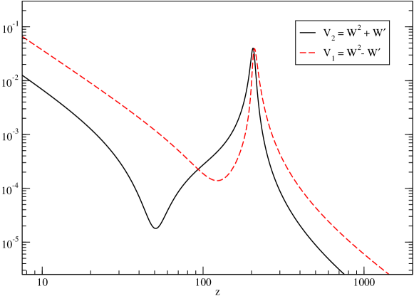
Figure 4: Superpartner potentials $V_{1}$ and $V_{2}$ for the eight-dimensional hypermonopole of Sec. 2. Although they do not support bound states, metastable massive gravitons are trapped in the confining nest around $z\simeq 200$. The peaks are associated with the regions of maximum curvature of Fig. 1 (same parameters).

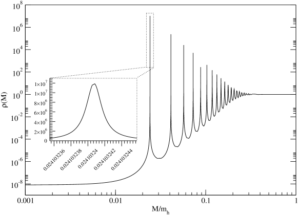
Figure 5: Spectral density with respect to the graviton mass for the eight-dimensional hypermonopole. The resonances correspond to the massive metastable states associated with the potential $V_{2}(z)$ plotted in Fig. 4. More than fifteen gravitons end up being trapped. The constant behaviour at small and large distances shows that gravity is $N$-dimensional in these regions, albeit with a different effective Newton constant due to the gravitational redshift.

Since the extra-dimensions are asymptotically flat, the mode functions far from the hypermonopole core are of the form given by Eq. (54). Using these Bessel wave-form as asymptotic initial conditions, we have numerically solved Eq. (44) in the background fields of Fig. 1. In Fig. 4, we have represented the superpartner potential $V_{1}$ and $V_{2}$ as a function of the conformal radial distance $z$. Solving for the mode equation in $V_{2}(z)$ gives the spectral density plotted in Fig. 5. For this configuration, we have observed more than fifteen trapped gravitons, the lightest having a spectral density profile typical of a Breit–Wigner distribution

$$\rho(M)\underset{m_{\mathrm{g}}}{\simeq}\frac{\displaystyle I}{\displaystyle 1+\left(\frac{\displaystyle M-m_{\mathrm{g}}}{\displaystyle\gamma_{\mathrm{g}}}\right)^{2}}\,,$$ (69)

whose best fit gives

$$m_{\mathrm{g}} = 2.4103240725\times 10^{-2}m_{\mathrm{h}},$$

$$\gamma_{\mathrm{g}} = 1.12\times 10^{-9}m_{\mathrm{h}}$$

$$I = 1.19\times 10^{7}.$$ (70)

In order to properly resolve the width of these resonance, we have implemented a recursive local adaptive mesh refinement coupled to the more usual Runge–Kutta integration of Eq. (44). For such very thin resonances, the toy model of Eq. (66) is a good approximation for $M\simeq m_{\mathrm{g}}$, the constant $C$ being given by the integral of Eq. (69). One finds

$$C=I\frac{\displaystyle\gamma_{\mathrm{g}}}{\displaystyle 2m_{\mathrm{g}}}\left(\pi+2\arctan\frac{\displaystyle m_{\mathrm{g}}}{\displaystyle\gamma_{\mathrm{g}}}\right)\simeq\pi I\frac{\displaystyle\gamma_{\mathrm{g}}}{\displaystyle m_{\mathrm{g}}}\,,$$ (71)

where the last expression is accurate only for $\gamma_{\mathrm{g}}\ll m_{\mathrm{g}}$. For the best fit values of Eq. (3.3), one finds $C\simeq 1.7$. As can be seen in Fig. (5), for light masses $\rho(M)=\varrho_{0}=8.2\times 10^{-9}$ such that the lower bound in Eq. (68) is about $10^{-2}$. We therefore expect this resonance to change the standard eight-dimensional gravity law on distances covering not more that two-orders of magnitude around the scale $1/m_{\mathrm{g}}$, which is far to short to be interesting for cosmological purpose.

However, we do not see any reasons preventing the existence of cosmologically interesting solutions, i.e. much lighter gravitons. Indeed, increasing $\alpha$ appears to push up the potential barrier in Fig. 4 whereas reducing $\epsilon$ increases the width of the potential barrier. Small values of $\epsilon$ have the effect of delocalising the gauge field and this ends up spreading its energy density over the extra-dimensions. Both of these parameters could therefore be somehow adjusted to obtained much lighter graviton resonances. As the numbers reported in Eq. (3.3) suggest, the precise determination of lighter resonances is made difficult due to numerical limitations, the machine precision accuracy not covering more than $16$ orders of magnitude on usual computers is already saturated by $\gamma_{\mathrm{g}}/I$ in Eq. (3.3).

3.4 Deviations from Newton

3.4.1 Dimensional reduction

In order to complete the discussion of the previous section, we have computed the Laplace transform directly from the spectral density found in Fig. 5.

Figure 6: Rescaled Laplace transform in linear (left) and logarithmic scale (right) associated with the spectral density of Fig. 5 and plotted as a function of the distance to the source. The Newton law is eight-dimensional when this quantity is constant as it occurs on small and large distances. The lightest graviton resonance of Eq. (3.3) reduces locally the dimensionality of the Newton force by a fractional power of exponent $2.4$ (best fit). The strong variation in amplitude from small to large scales comes from the hypermonopole induced gravitational redshift.

Fig. 6 shows the rescaled quantity $|\vec{x}|^{n+1}\mathcal{L}_{|\vec{x}|}\negthinspace\left\{M^{n}\rho(M)\right\}$ as a function of the distance to the source. Gravity is $N$-dimensional when this quantity is constant as it occurs at small and large distances. The strong variation in amplitude, also visible in the smooth change of the spectral density in Fig. 5, comes again from the hypermonopole gravitational redshift (see the $\sigma$ profile in Fig. 1). The graviton resonance of Eq. (3.3) is responsible of the peak located around $x\simeq 1/m_{\mathrm{g}}$. A best power fit of the potential nearby this region shows that the Newton law is dimensionally reduced to $1/x^{3.6}$. This is not yet a four-dimensional Newton law due to the previously discussed numerical limitations to obtain a light enough resonance.

3.4.2 Effective gravitational coupling

From Eqs. (62), (64) and (67), one can extract the effective Newton constant $G$ which would be measured by a four-dimensional observer in the three expected regimes. At very small distances,

$$|\Delta\vec{x}|m_{\mathrm{g}}\ll\left(\frac{\displaystyle\varrho_{0}\Gamma(n+1)}{\displaystyle C}\right)^{1/(n+1)},$$ (72)

the spectral density is constant $\rho(M)=1$ and thus gravity is seven dimensional. The measured Newton constant is however reduced by the dilaton condensation in the hypermonopole core:

$$G_{0}=e^{-\psi(0)}G_{N}\,.$$ (73)

In the intermediate regions, those verifying Eq. (68), gravity is driven by the metastable lightest graviton and the Newton law is four-dimensional with an effective Newton constant given by

$$G_{4}=e^{-\psi(0)}\frac{\displaystyle G_{N}}{\displaystyle 2}\frac{\displaystyle n+3}{\displaystyle n+2}\frac{\displaystyle C}{\displaystyle\Gamma(n+1)}m_{\mathrm{g}}^{n+1}.$$ (74)

This equation makes clear that a light graviton, required for the dimensional reduction of the Newton law, will necessarily induce a small effective Newton constant thereby addressing the mass hierarchy problem. In terms of the reduced Planck masses, Eq. (74) can be recast into

$$M_{\mathrm{Pl}}^{2}=2e^{\psi(0)}\frac{\displaystyle n+2}{\displaystyle n+3}\frac{\displaystyle\Gamma(n+1)}{\displaystyle C}\frac{\displaystyle M^{n+3}}{\displaystyle m_{\mathrm{g}}^{n+1}}\,,$$ (75)

where $M_{\mathrm{Pl}}^{2}=1/G_{4}$ and $M^{N-2}=1/G_{N}$.

Finally, on the largest length scales,

$$|\Delta\vec{x}|m_{\mathrm{g}}\gg 1,$$ (76)

gravity becomes again $N$-dimensional but with a much weaker Newton constant since now $\rho(M\rightarrow 0)=\varrho_{0}\ll 1$. The measured Newton constant is now given by

$$G_{\infty}=\varrho_{0}e^{-\psi(0)}G_{N}=\varrho_{0}G_{0}\ll G_{0}.$$ (77)

As a numerical application, we can determine the order of magnitude of the $N$-dimensional Planck mass such that the graviton mass is of the same order than the cosmological constant energy scale, i.e. $m_{\mathrm{g}}\simeq 10^{-11}\mathrm{GeV}$. From Eq. (75), one gets

$$M\simeq\left[\frac{\displaystyle Ce^{-\psi(0)}}{\displaystyle\Gamma(n+1)}\right]^{1/(n+3)}\times 10^{\frac{25-11n}{n+3}}\mathrm{GeV},$$ (78)

which is down to the $10\,\mathrm{GeV}$ scale already for $n=2$. Notice that the lowest scale at which $N$-dimensional gravity shows up is fixed by the value of $\varrho_{0}$ and not by $m_{\mathrm{g}}$. This quantity coming only from the gravitational redshift $\sigma(0)$, it can actually be made arbitrarily small for order one coupling constants, i.e. for Higgs vacuum expectation values also around the $10\,\mathrm{GeV}$ scale. In fact, as suggested by the previous equation, the mass hierarchy mechanism advocated here is so efficient that it has a natural preference for very small $N$-dimensional Planck masses.

4 Conclusion

In this paper we have shown that metastable massive gravitons generically exist in the four-dimensional core of any self-gravitating hypermonopoles formed by the breakdown of an $SO(n_{\mathrm{e}})$ symmetry in $(n_{\mathrm{e}}+4)$ dimensions, provided $n_{\mathrm{e}}\geq 3$.

Since the extra-dimensional spacetime is of infinite volume and asymptotically flat, these resonances induce a DGP-like gravity confinement mechanism in the core. For light enough resonances, gravity is $N$-dimensional at small and large distances, but can be four-dimensional on some intermediate range. The numerical determination of such a light and long-lived resonance may be however a non-trivial problem due to finite numerical accuracy. Moreover, we have shown that, in this regime, the effective four-dimensional Planck mass is proportional to an inverse power of the graviton mass; this one being extremely light, the mass hierarchy problem ends up being naturally addressed in our setup. The strong decay of the gravity law at large distances, coming from both the higher-dimensionality and the strong gravitational redshift, might be of interest to explain the current cosmic acceleration.

Finally, we would like to emphasize that these models still remain unexplored on various aspects which may compromise, or not, their viability. Here, we have only solved the propagation of spin two fluctuations which decouple from the background fields. The model has however vector and scalar modes which may propagate and might also be confined in the core. Solving for their propagation is a challenging problem since they will be necessarily coupled to all of hypermonopole-forming vector and scalar fields. We leave the second order perturbation of Eq. (3) in the scalar and vector modes for a future work.

5 Appendix

In this appendix, we present the Einstein tensor $G_{AB}$ and the stress tensor $T_{AB}$. Inserted into Eq. (8), we then arrive at the equations of motion for the gravity sector (26), (27) and (28). For the metric given in Eq. (14), the Einstein tensor is given by

$$G_{\mu\nu} = m_{\mathrm{h}}^{2}g_{\mu\nu}\left[\frac{3}{2}\ddot{\sigma}+\frac{3}{2}\dot{\sigma}^{2}+n\frac{\ddot{\varpi}}{\varpi}+\frac{n(n-1)}{2}\left(\frac{\dot{\varpi}}{\varpi}\right)^{2}\frac{3n}{2}\frac{\dot{\sigma}\dot{\varpi}}{\varpi}-\frac{n(n-1)}{2\varpi^{2}}\right],$$

$$G_{rr} = m_{\mathrm{h}}^{2}\left[\frac{3}{2}(\dot{\sigma})^{2}+\frac{n(n-1)}{2}\left(\frac{\dot{\varpi}}{\varpi}\right)^{2}+2n\frac{\dot{\sigma}\dot{\varpi}}{\varpi}-\frac{n(n-1)}{2\varpi^{2}}\right],$$

$$G_{\theta_{i}\theta_{j}} = m_{\mathrm{h}}^{2}g_{\theta_{i}\theta_{j}}\left[2\ddot{\sigma}+\frac{5}{2}(\dot{\sigma})^{2}+(n-1)\frac{\ddot{\varpi}}{\varpi}\right.$$ (79)

$$+ \left.2(n-1)\frac{\dot{\sigma}\dot{\varpi}}{\varpi}\frac{(n-1)(n-2)}{2}\left(\frac{\dot{\varpi}}{\varpi}\right)^{2}-\frac{(n-1)(n-2)}{2\varpi^{2}}\right].$$

With the Higgs and gauge fields specified by Eqs. (17), (24) and (21), the stress tensor (10) becomes

$$T_{\mu\nu} = \frac{v^{2}m_{\mathrm{h}}^{2}}{2}g_{\mu\nu}\left[-\dot{f}^{2}-n\left(\frac{fQ}{\varpi}\right)^{2}-\frac{n}{\epsilon\varpi^{2}}\dot{Q}^{2}-\frac{n(n-1)}{2\epsilon\varpi^{4}}(1-Q^{2})^{2}\right.$$

$$- \left.\frac{1}{4}(f^{2}-1)^{2}\right],$$

$$T_{rr} = \frac{v^{2}m_{\mathrm{h}}^{2}}{2}\left[\dot{f}^{2}+\frac{n}{\epsilon\varpi^{2}}\dot{Q}^{2}-n\left(\frac{fQ}{\varpi}\right)^{2}-\frac{n(n-1)}{2\epsilon\varpi^{4}}(1-Q^{2})^{2}\right.$$

$$- \left.\frac{1}{4}(f^{2}-1)^{2}\right],$$

$$T_{\theta_{i}\theta_{j}} = \frac{v^{2}m_{\mathrm{h}}^{2}}{2}g_{\theta_{i}\theta_{j}}\left[-\dot{f}^{2}-(n-2)\left(\frac{fQ}{\varpi}\right)^{2}\right.$$ (80)

$$- \left.\frac{n-2}{\epsilon\varpi^{2}}\dot{Q}^{2}-\frac{(n-1)(n-4)}{2\epsilon\varpi^{4}}(1-Q^{2})^{2}-\frac{1}{4}(f^{2}-1)^{2}\right].$$

References

References

• [1] G. Nordstrom, On the possibility of unifying the electromagnetic and the gravitational fields, Phys. Z. 15 (1914) 504–506, [physics/0702221].
• [2] T. Kaluza, Zum Unitätsproblem in der Physik, Sitzungsber. Preuss. Akad. Wiss. Berlin (1921) 966.
• [3] O. Klein, Quantum theory and five-dimensional theory of relativity, Z. Phys. 37 (1926) 895–906.
• [4] I. Antoniadis, A Possible new dimension at a few TeV, Phys. Lett. B246 (1990) 377–384.
• [5] P. Horava and E. Witten, Heterotic and type i string dynamics from eleven dimensions, Nucl. Phys. B460 (1996) 506–524, [http://arXiv.org/abs/hep-th/9510209].
• [6] A. Lukas, B. A. Ovrut, and D. Waldram, Cosmological solutions of horava-witten theory, Phys. Rev. D60 (1999) 086001, [hep-th/9806022].
• [7] N. Arkani-Hamed, S. Dimopoulos, and G. R. Dvali, The hierarchy problem and new dimensions at a millimeter, Phys. Lett. B429 (1998) 263–272, [hep-ph/9803315].
• [8] I. Antoniadis, N. Arkani-Hamed, S. Dimopoulos, and G. R. Dvali, New dimensions at a millimeter to a Fermi and superstrings at a TeV, Phys. Lett. B436 (1998) 257–263, [hep-ph/9804398].
• [9] L. Randall and R. Sundrum, A large mass hierarchy from a small extra dimension, Phys. Rev. Lett. 83 (1999) 3370–3373, [hep-ph/9905221].
• [10] R. Gregory, V. A. Rubakov, and S. M. Sibiryakov, Opening up extra dimensions at ultra-large scales, Phys. Rev. Lett. 84 (2000) 5928–5931, [hep-th/0002072].
• [11] C. Ringeval, P. Peter, and J.-P. Uzan, Localization of massive fermions on the brane, Phys. Rev. D65 (2002) 044016, [hep-th/0109194].
• [12] E. Fischbach, D. E. Krause, V. M. Mostepanenko, and M. Novello, New constraints on ultrashort-ranged Yukawa interactions from atomic force microscopy, Phys. Rev. D64 (2001) 075010, [hep-ph/0106331].
• [13] V. B. Bezerra, G. L. Klimchitskaya, V. M. Mostepanenko, and C. Romero, Advance and prospects in constraining the Yukawa-type corrections to Newtonian gravity from the Casimir effect, arXiv:1002.2141.
• [14] C. Deffayet, G. R. Dvali, and G. Gabadadze, Accelerated universe from gravity leaking to extra dimensions, Phys. Rev. D65 (2002) 044023, [astro-ph/0105068].
• [15] L. Randall and R. Sundrum, An alternative to compactification, Phys. Rev. Lett. 83 (1999) 4690–4693, [hep-th/9906064].
• [16] G. R. Dvali, G. Gabadadze, and M. Porrati, 4d gravity on a brane in 5d minkowski space, Phys. Lett. B485 (2000) 208–214, [hep-th/0005016].
• [17] G. R. Dvali and G. Gabadadze, Gravity on a brane in infinite-volume extra space, Phys. Rev. D63 (2001) 065007, [hep-th/0008054].
• [18] C. Deffayet, G. Gabadadze, and A. Iglesias, Perturbations of self-accelerated universe, JCAP 0608 (2006) 012, [hep-th/0607099].
• [19] R. Gregory, N. Kaloper, R. C. Myers, and A. Padilla, A New Perspective on DGP Gravity, JHEP 10 (2007) 069, [arXiv:0707.2666].
• [20] G. Gabadadze and M. Shifman, Softly massive gravity, Phys. Rev. D69 (2004) 124032, [hep-th/0312289].
• [21] N. Kaloper and D. Kiley, Charting the Landscape of Modified Gravity, JHEP 05 (2007) 045, [hep-th/0703190].
• [22] N. Kaloper, Brane Induced Gravity: Codimension-2, Mod. Phys. Lett. A23 (2008) 781–796, [arXiv:0711.3210].
• [23] G. Dvali, S. Hofmann, and J. Khoury, Degravitation of the cosmological constant and graviton width, Phys. Rev. D76 (2007) 084006, [hep-th/0703027].
• [24] C. de Rham, S. Hofmann, J. Khoury, and A. J. Tolley, Cascading Gravity and Degravitation, JCAP 0802 (2008) 011, [arXiv:0712.2821].
• [25] C. de Rham et. al., Cascading gravity: Extending the Dvali-Gabadadze-Porrati model to higher dimension, Phys. Rev. Lett. 100 (2008) 251603, [arXiv:0711.2072].
• [26] C. de Rham, J. Khoury, and A. J. Tolley, Flat 3-Brane with Tension in Cascading Gravity, Phys. Rev. Lett. 103 (2009) 161601, [arXiv:0907.0473].
• [27] C. de Rham, J. Khoury, and A. J. Tolley, Cascading Gravity is Ghost Free, arXiv:1002.1075.
• [28] M. Kolanovic, M. Porrati, and J.-W. Rombouts, Regularization of brane induced gravity, Phys. Rev. D68 (2003) 064018, [hep-th/0304148].
• [29] M. Kolanovic, Gravity induced over a smooth soliton, Phys. Rev. D67 (2003) 106002, [hep-th/0301116].
• [30] M. Shaposhnikov, P. Tinyakov, and K. Zuleta, Quasilocalized gravity without asymptotic flatness, Phys. Rev. D70 (2004) 104019, [hep-th/0411031].
• [31] C. Ringeval and J.-W. Rombouts, Metastable gravity on classical defects, Phys. Rev. D71 (2005) 044001, [hep-th/0411282].
• [32] A. De Felice and C. Ringeval, Massive gravitons trapped inside a hypermonopole, Phys. Lett. B671 (2009) 158–161, [arXiv:0809.0464].
• [33] K. Akama, An early proposal of ’brane world’, Lect. Notes Phys. 176 (1982) 267–271, [hep-th/0001113].
• [34] V. A. Rubakov and M. E. Shaposhnikov, Do we live inside a domain wall?, Phys. Lett. B125 (1983) 136–138.
• [35] M. Visser, An exotic class of Kaluza-Klein models, Phys. Lett. B159 (1985) 22, [hep-th/9910093].
• [36] G. W. Gibbons and D. L. Wiltshire, Space-Time as a Membrane in Higher Dimensions, Nucl. Phys. B287 (1987) 717, [hep-th/0109093].
• [37] M. Cvetic and H. H. Soleng, Supergravity domain walls, Phys. Rept. 282 (1997) 159–223, [hep-th/9604090].
• [38] R. M. Wald, General Relativity. Univ. Pr., Chicago, 1984.
• [39] E. Roessl and M. Shaposhnikov, Localizing gravity on a ’t hooft-polyakov monopole in seven dimensions, Phys. Rev. D66 (2002) 084008, [hep-th/0205320].
• [40] C. Ringeval, P. Peter, and J.-P. Uzan, Stability of six-dimensional hyperstring braneworlds, Phys. Rev. D71 (2005) 104018, [hep-th/0301172].
• [41] S. M. Carroll, J. Geddes, M. B. Hoffman, and R. M. Wald, Classical stabilization of homogeneous extra dimensions, Phys. Rev. D66 (2002) 024036, [hep-th/0110149].
• [42] T. Kibble, Topology of cosmic domains and strings, J. Phys. A9 (1976) 1387.
• [43] G. ’t Hooft, Magnetic monopoles in unified gauge theories, Nucl. Phys. B79 (1974) 276–284.
• [44] A. M. Polyakov, Particle spectrum in quantum field theory, JETP Lett. 20 (1974) 194.
• [45] J. R. Cash and F. Mazzia, A new mesh selection algorithm, based on conditioning, for two-point boundary value codes, J. Comput. Appl. Math. 184 (2005), no. 2 362–381.
• [46] F. Cooper, A. Khare, and U. Sukhatme, Supersymmetry and quantum mechanics, Phys. Rept. 251 (1995) 267–385, [hep-th/9405029].
• [47] I. S. Gradshteyn and I. M. Ryzhik, Table of Integrals, Series, and Products. Academic Press, New York and London, 1965.
• [48] M. Abramowitz and I. A. Stegun, Handbook of mathematical functions with formulas, graphs, and mathematical tables. National Bureau of Standards, Washington, US, ninth ed., 1970.