Classical Phase Transitions of Geometrically Constrained O($N$) Spin Systems

Abstract

We study the phase transition between the high temperature algebraic liquid phase and the low temperature ordered phase in several different types of locally constrained O($N$) spin systems, using a unified constrained Ginzburg-Landau formalism. The models we will study include: $\mathbf{1}$, O($N$) spin-ice model with cubic symmetry; $\mathbf{2}$, O($N$) spin-ice model with easy-plane and easy-axis anisotropy; $\mathbf{3}$, a novel O($N$) “spin-plaquette” model, with a very different local constraint from the spin-ice. We calculate the renormalization group equations and critical exponents using a systematic $\epsilon=4-d$ expansion with constant $N$, stable fixed points are found for large enough $N$. In the end we will also study the situation with softened constraints, the defects of the constraints will destroy the algebraic phase and play an important role at all the transitions.

I I, introduction

It is well-known that sometimes constraints imposed locally can lead to stable phases with unusual long distance correlations. For instance, at zero temperature the local constraints can give rise to quantum Bose liquid phase with gapless excitations analogous to photon or even graviton Moessner and Sondhi (2003a); Hermele et al. (2004); Wen (2003); Xu (2006a, b). At finite temperature, in three dimensional classical dimer model (CDM) and spin-ice systems, the local geometric constraint grants the high temperature spin disordered phase an algebraic power-law correlation between dimer and spin densities Isakov et al. (2005); Castelnovo et al. (2008); Huse et al. (2003); Chen et al. (2009); Alet et al. (2006); Misguich et al. (2008), instead of the standard short-range correlations according to the Ginzburg-Landau theory. This algebraic phase is usually called the Coulomb phase. In both the dimer models and spin-ices, physical quantities are defined on links of a bipartite lattice, and let us take the cubic lattice for simplicity. The ensemble of 3d CDM is all the configurations of dimer coverings, which are subject to a local constraint on every site: each site is connected to precisely $m$ dimers with $0<m<6$ (denoted as CDM-$m$), and most studies have been focused on the case with $m=1$. The ensemble of the spin-ice model is all the configurations of spins on the links, and the sum of the six spin vectors around each site is zero, which is usually called the ice-rule Pauling (1935). Although the spin is generically an O(3) vector, due to the spin-orbit coupling, the spins in the spin-ice materials prefer to align along the links where the spins reside, therefore people usually treat the spins in spin-ice materials Ising spins Castelnovo et al. (2008), hence the spin-ice model on the cubic lattice is mathematically equivalent to CDM-3. The power-law correlation of the Coulomb phase has been confirmed by numerical simulations Chen et al. (2009); Alet et al. (2006); Misguich et al. (2008) and also neutron scattering in spin-ice materials such as $\mathrm{Ho_{2}Ti_{2}O_{7}}$ and $\mathrm{Dy_{2}Ti_{2}O_{7}}$ Fennell et al. (2009).

The partition function of the CDM-$m$ is a sum of all the dimer configurations allowed by the constraint, with a Boltzmann weight that favors certain dimer configurations. To describe CDM-$m$ concisely, we can introduce the “magnetic field” $B_{i,\mu}=(n_{i,\mu}-m/6)\eta_{i}$ with $\mu=+\hat{x},+\hat{y},+\hat{z}$, where $\eta_{i}=(-1)^{i}$ is a staggered sign distribution on the cubic lattice. The number $n_{i,\mu}$ is defined on each link $(i,\mu)$ between sites $i$ and $i+\mu$, and $n_{i,\mu}=1,\ 0$ represents the presence and absence of dimer. Now the local constraint of the dimer system can be rewritten as a Gauss law constraint $\vec{\nabla}\cdot\vec{B}=0$. The standard way to solve this Gauss law constraint is to introduce vector potential $\vec{A}$ defined on the unit plaquettes of the cubic lattice, and $\vec{B}=\vec{\nabla}\times\vec{A}$ Moessner and Sondhi (2003b); Hermele et al. (2005). Since vector $\vec{A}$ is no longer subject to any constraint, it is usually assumed that at low energy the system can be described by a local field theory of $\vec{A}$, for instance the low energy field theory of the Coulomb phase reads

$$F\sim\int d^{3}x(\vec{\nabla}\times\vec{A})^{2}+\cdots$$ (1)

which is invariant under gauge transformation $\vec{A}\rightarrow\vec{A}+\vec{\nabla}f$, $f$ is an arbitrary function of space. In the Coulomb phase, the correlation of magnetic field $B_{\mu}$ in the momentum space reads

$$\langle B_{\mu}(\vec{q})B_{\nu}(-\vec{q})\rangle\sim\delta_{\mu\nu}-\frac{q_{\mu}q_{\nu}}{q^{2}}.$$ (2)

The spin-ice model can be straightforwardly generalized to the O($N$) case. We can define an O($N$) spin vector $S^{a}$ with unit length $\sum_{a}(S^{a})^{2}=1$ on each link $(i,\mu)$ of the cubic lattice (Fig. 2$a$), with $a=1\cdots N$, and we assume that the largest term of the Hamiltonian imposes an ice-rule constraint Pauling (1935) for O($N$) spins on the six links shared by every site:

$$\sum_{\mu=x,y,z}S^{a}_{i,\mu}+S^{a}_{i-\mu,\mu}=0.$$ (3)

The magnetic field formalism developed for the CDM can be naturally applied here, with $\phi^{a}_{i,\mu}=\eta_{i}S^{a}_{i,+\mu}$, and the constraint Eq. 3 can be written as

$$\sum_{\mu}\nabla_{\mu}\phi^{a}_{\mu}=0.$$ (4)

Then in the Coulomb phase the momentum space correlation between $\phi^{a}_{\mu}$ reads

$$\langle\phi^{a}_{\mu}(\vec{q})\phi^{b}_{\nu}(-\vec{q})\rangle\sim\delta_{ab}(\delta_{\mu\nu}-\frac{q_{\mu}q_{\nu}}{q^{2}}),$$ (5)

which after Fourier transformation leads to the same $1/r^{3}$ power-law correlation as the dimer model.

Another constrained spin system, which is very different from the spin-ice is the classical plaquette model (CPM). In Ref. Pankov et al. (2007); Xu and Wu (2008) a plaquette model engineered from the SU(4) Heisenberg model on the cubic lattice was studied, and one of the twelve unit square faces shared by each site of the cubic lattice is occupied by a plaquette, which is physically the SU(4) singlet formed by four fermions at the corners. The exact SU(4) symmetry can be realized in cold atom system without fine-tuning Wu et al. (2003); Gorshkov et al. (2009). The ensemble of the CPM-$m$ is all the plaquette configurations on the cubic lattice, with exactly $m$ plaquettes shared by each site (Fig. 2$b$). To generalize this system to O($N$), let us define O($N$) spins $S^{a}$ on the unit faces instead of the links of the cubic lattice, and impose the constraint that the sum of spin vectors on all the twelve faces shared by every site be zero (Fig. 2$c$). When $N=1$, this model is equivalent to CPM-6. In this case it is most convenient to introduce symmetric rank-2 tensor $\phi^{a}_{i,\mu\nu}=\eta_{i}S^{a}_{i,\mu\nu}$ with $\mu,\nu=+\hat{x},+\hat{y},+\hat{z}$. $(i,\mu\nu)$ denotes the unit square face shared by sites $i$, $i+\mu$, $i+\nu$ and $i+\mu+\nu$. In terms of $\phi^{a}_{\mu\nu}$, the spin plaquette constraint can be written as

$$\sum_{\mu\neq\nu}\nabla_{\mu}\nabla_{\nu}\phi^{a}_{\mu\nu}=0.$$ (6)

This spin-plaquette system also has an algebraic phase at finite temperature, with the following momentum space correlation:

$$\langle\phi^{a}_{\mu\nu}(\vec{q})\phi^{b}_{\rho\sigma}(-\vec{q})\rangle \sim \delta_{ab}(\delta_{\mu\rho}\delta_{\nu\sigma}+\delta_{\mu\sigma}\delta_{\nu\rho}$$ (7)

$$- \frac{q_{\mu}q_{\nu}q_{\rho}q_{\sigma}}{q_{x}^{2}q_{y}^{2}+q_{y}^{2}q_{z}^{2}+q_{x}^{2}q_{z}^{2}}).$$ (9)

Besides the high temperature algebraic phases in the models discussed above, at low temperature spins are expected to order according to the details of the Hamiltonian. In this work we will study the phase transition between the high temperature algebraic phase and the low temperature spin ordered phase in O($N$) spin-ice (section II), with both cubic symmetry and anisotropies, as well as O($N$) spin-plaquette system (section III). In section IV we will study the situation with softened constraints. The nature of the transitions clearly depend on the low temperature spin order pattern, and in this work we will focus on one particular type of spin order, which has nonzero net $\langle\phi^{a}_{\mu}\rangle$ and $\langle\phi^{a}_{\mu\nu}\rangle$ at large length scale. Our calculation will be based on $\epsilon=4-d$ expansion. Due to the complexity of the calculation, in our current work we will keep the precision to the first order $\epsilon$ expansion.

II II, O($N$) spin-ice model

II.1 A, Brief Review of the CDM

Let us first give a brief review of the previously studied phase transition of the CDM, or the spin-ice model with $N=1$. The field theory Eq. 1 misses one important piece of information: the magnetic field $\vec{B}$ and the vector potential $\vec{A}$ are both discrete. Therefore mathematically we should introduce “vertex operator” $L_{v}\sim\sum_{\mu}\cos[2\pi(A_{\mu}+\tilde{a}_{\mu})]$ to the field theory Eq. 1, and $\tilde{a}_{\mu}$ is a nonzero background distribution of the vector potential, which is introduced for any nonzero $m$. The Coulomb phase is a phase where this vertex operator is irrelevant perturbatively. The vertex operator will become nonperturbative and drive a phase transition when it is large, and in order to describe this phase transition one can introduce matter fields in the vertex operator which couple to the gauge field minimally:

$$L_{v}\sim\sum_{\mu}\cos[2\pi(\nabla_{\mu}\theta-A_{\mu}-\tilde{a}_{\mu})],$$ (10)

$\theta$ is the phase angle of the matter field $\psi\sim e^{i\theta}$. Due to the existence of the nonzero $\tilde{a}_{\mu}$, the matter fields $\psi$ move on a nonzero background magnetic field, the band structure of the matter fields have multiple minima in the Brillouin zone, and the transformation between these minima encodes the information of the lattice symmetry Motrunich and Senthil (2005). Therefore in addition to manifesting the discrete nature of the gauge potential $A_{\mu}$, the condensation of the matter field leads to lattice symmetry breaking, which corresponds to the crystal phase of the CDM. For instance the transition between the Coulomb and columnar crystal phases of the CDM-1 model is described by the CP(1) model with an enlarged SU(2) global symmetry Powell and Chalker (2008); Chen et al. (2009). This field theory is highly unconventional, in the sense that it is not formulated in terms of physical order parameters. It is expected that more general CDM-$m$ models can also be described by similar Higgs transition, although the detailed lattice symmetry transformation for matter fields would depend on $m$.

One might be tempted to describe the transition between the Coulomb and columnar phases of CDM-1 trough a Ginzburg-Landau approach. One can introduce an O(3) vector $\vec{\varphi}$ with cubic symmetry anisotropy in favor of six axial directions, and $\langle\varphi_{\mu}\rangle\sim\pm 1$ represents six fold degenerate columnar order. However, the hedgehog monopole configuration of the O(3) vector $\vec{\varphi}$ always involves a broken dimer $i.e.$ a defect of the constraint. Then as long as we forbid the presence of the defects, this O(3) model is monopole-free, and it is well-known that the monopole-free O(3) nonlinear sigma model is equivalent to the CP(1) model Motrunich and Vishwanath (2004), which has very different critical exponents from the O(3) Wilson-Fisher fixed point Kamal and Murthy (1993); Motrunich and Vishwanath (2009).

II.2 B, Isotropic O($N$) Spin-ice

When $N>1$, the spin takes continuous values, therefore the formalism of the phase transition based on vertex operator in the previous section is no longer applicable. Also, it is impossible to write down a vertex operator with the O($N$) spin symmetry. Therefore, we need to seek for a different formalism. We consider the following Hamiltonian for O($N$) spin-ice in addition to the dominant constraint Eq. 3:

$$E = \sum_{i,\mu,a}J_{1}S^{a}_{i-\mu,\mu}S^{a}_{i,\mu}+\sum_{i,a}\sum_{\mu\neq\nu}J_{2}S^{a}_{i,\mu}S^{a}_{i+\nu,\mu}.$$ (11)

$J_{1}$ is a Heisenberg coupling between spins along the same lattice axis, $J_{2}$ is a Heisenberg coupling between spins on two parallel links across a unit square face. If $J_{1}>0$ and $J_{2}<0$, in the ground state spins are antiparallel along the same axis, but parallel between parallel links across a unit square $i.e.$ $\langle S^{a}_{i+\mu}\rangle\sim(-1)^{i_{\mu}}\mathcal{S}^{a}_{\mu}$, $\mathcal{S}^{a}_{\mu}$ is a constant O($N$) vector. Using the CDM terminology, we will call this state the columnar state. If $J_{1}$ and $J_{2}$ are both positive, in the ground state the spins are antiparallel between nearest neighbor links on the same axis, as well as between parallel links across a unit square ($\langle S^{a}_{i+\mu}\rangle\sim(-1)^{i}\mathcal{S}^{a}_{\mu}$), and we will call this state the staggered state. Since in the $J_{1}-J_{2}$ model Eq. 11 there is no coupling between different axes along different directions, for both cases the zero temperature ground state of model Eq. 11 has large degeneracy, because the energy does not depend on the relative angle between $\mathcal{S}^{a}_{i,x}$, $\mathcal{S}^{a}_{i,y}$ and $\mathcal{S}^{a}_{i,z}$ $i.e.$ the ground state manifold has an enlarged $[\mathrm{O}(N)]^{3}$ symmetry. However, at finite temperature this accidental enlarged symmetry of the ground state will be broken due to thermal fluctuation.

In this paper we will focus on the staggered spin order. Following the magnetic field formalism of the CDM mentioned before, in order to describe this system compactly, we introduce three flavors of O($N$) vector field $\phi^{a}_{\mu}=S^{a}_{i,+\mu}\eta_{i}$ with $\mu=x,y,z$, and now the constraint Eq. 3 can be rewritten concisely as

$$\sum_{\mu}\nabla_{\mu}\phi^{a}_{\mu}=0.$$ (12)

Under the lattice symmetry transformation, $\phi^{a}_{\mu}$ transforms as

$$T_{\mu} : \ \mu\rightarrow\mu+1,\ \phi^{a}_{\nu}\rightarrow-\phi^{a}_{\nu},\ (\mathrm{for}\ \mathrm{all}\ \mu,\ \nu),$$ (13)

$$R_{\mu,s} : \ \mu\rightarrow-\mu,\ \phi^{a}_{\mu}\rightarrow-\phi^{a}_{\mu},\ \phi^{a}_{\nu}\rightarrow\phi^{a}_{\nu},\ (\mathrm{for}\ \nu\neq\mu),$$ (15)

$$R_{\mu\nu} : \ \mu\leftrightarrow\nu,\ \phi^{a}_{\mu}\leftrightarrow\phi^{a}_{\nu},\ (\mathrm{for}\ \nu\neq\mu).$$ (17)

$T_{\mu}$ is the translation symmetry along $\mu$ direction, $R_{\mu,s}$ is the site centered reflection symmetry, and $R_{\mu\nu}$ is the reflection along a diagonal direction.

The staggered spin order corresponds to the uniform order of $\phi^{a}_{\mu}$, and all flavors of spin vectors are ordered. Therefore presumably $\phi^{a}_{\mu}$ are the low energy modes close to the transition, and we can write down the following symmetry allowed trial field theory for $\phi^{a}_{\mu}$ with softened unit length constraint:

$$\mathcal{F} = \sum_{\mu,a}\phi^{a}_{\mu}(-\nabla^{2}+r-\gamma\nabla_{\mu}^{2})\phi^{a}_{\mu}$$ (18)

$$+ \sum_{a}g(\sum_{\mu}\nabla_{\mu}\phi^{a}_{\mu})^{2}+\mathcal{F}_{4}$$ (20)

When we take $g\rightarrow\infty$, the constraint Eq. 12 is effectively imposed. In Eq. 20 when $\gamma=0$, the quadratic part of the field theory is invariant under $\mathrm{O}(N)\times\mathrm{O}(3)$ transformation, the O(3) symmetry is a combined flavor-orbital rotation symmetry. $\gamma$ term will break this symmetry down to the cubic lattice symmetry and O($N$) spin symmetry. The flow of $\gamma$ comes from the two loop self-energy correction diagram (Fig. 1$d$), and the RG flow of $\gamma$ will contribute to the RG equation at the order of $\epsilon^{3}$, which is negligible at the accuracy of our calculation if we take $\epsilon=4-d$ small. Therefore $\gamma$ is a constant instead of a scaling function in the RG equation, hereafter we will always assume $\gamma$ is small.

$\mathcal{F}_{4}$ in Eq. 20 includes all the symmetry allowed quartic terms of $\phi^{a}_{\mu}$:

$$\mathcal{F}_{4} = u\sum_{\mu}[\sum_{a}(\phi^{a}_{\mu})^{2}]^{2}+v\sum_{\mu<\nu}[\sum_{a}(\phi^{a}_{\mu})^{2}][\sum_{b}(\phi^{b}_{\nu})^{2}]$$ (21)

$$+ w\sum_{\mu<\nu}[\sum_{a}\phi^{a}_{\mu}\phi^{a}_{\nu}][\sum_{b}\phi^{b}_{\mu}\phi^{b}_{\nu}].$$ (23)

The $u$ and $v$ terms are invariant under an enlarged symmetry $[\mathrm{O}(N)]^{3}$, while the $w$ term breaks this symmetry down to one single O($N$) symmetry plus lattice symmetry. As already mentioned, the ground state manifold of model Eq. 11 has the same enlarged $[\mathrm{O}(N)]^{3}$ symmetry. However, the $w$ term can be induced with thermal fluctuation through order-by-disorder mechanism Henley (1989), or we can simply turn on such extra bi-quadratic term energetically in the $J_{1}-J_{2}$ model Eq. 11. By adjusting the ratio between $u$, $v$ and $w$ in Eq. 23, points with various enlarged symmetry can be found. For instance, if $w+v=2u$, the $\mathcal{F}_{4}$ has a $\mathrm{O}(N)\times\mathrm{O}(3)$ symmetry, where the O(3) is the flavor-orbital combined rotation. Just like the $J_{1}-J_{2}$ model on the square lattice Henley (1989), the quadratic coupling $\sum_{a}\phi^{a}_{\mu}\phi^{a}_{\nu}$ with $\mu\neq\nu$ as well as more complicated quartic terms like $[\sum_{a}\phi^{a}_{x}\phi^{a}_{y}][\sum_{b}\phi^{b}_{y}\phi^{b}_{z}]$ break the reflection symmetry of the system, and hence are forbidden.

Figure 1: $(a)$, $(b)$ and $(c)$, momentum-shell loop integrals evaluated to be $A\ln(\Lambda/\tilde{\Lambda})$, $B\ln(\Lambda/\tilde{\Lambda})$ and $C\ln(\Lambda/\tilde{\Lambda})$ respectively, with parameters given by Eq. LABEL:abc. $(d)$, the self-energy correction that renormalizes $\gamma$ in Eq. 20, this two loop diagram will contribute to the renormalization of $u$, $v$ and $w$ at order $\epsilon^{3}$, and hence is negligible in our calculation.

If we just take the inverse of the Gaussian part of Eq. 20 with $r>0$, we obtain the following correlation function of $\phi^{a}_{\mu}$:

$$D^{ab}_{\mu\nu}\sim\frac{\delta_{ab}}{r+q^{2}}(\delta_{\mu\nu}-\frac{gq_{\mu}q_{\nu}}{r+(1+g)q^{2}}).$$ (24)

In the limit with $g\rightarrow\infty$, the correlation function reads

$$\lim_{g\rightarrow\infty}D^{ab}_{\mu\nu}(\vec{q}) = \langle\phi^{a}_{\mu}(\vec{q})\phi^{b}_{\nu}(-\vec{q})\rangle\sim\frac{\delta_{ab}}{r+q^{2}}P_{\mu\nu},$$ (25)

$$\ P_{\mu\nu} = \delta_{\mu\nu}-\frac{q_{\mu}q_{\nu}}{q^{2}}.$$ (27)

$P_{\mu\nu}$ is a projection matrix that projects a vector to the direction perpendicular to its momentum. After Fourier transformation, this correlation function gives us the $1/r^{3}$ power-law spin correlation of the Coulomb phase. When $r<0$, the vector $\phi^{a}_{\mu}$ is ordered. Interaction $\mathcal{F}_{4}$ will not spontaneously generate longitudinal spin wave. For instance, we can first keep $g$ finite at the beginning, and calculate the leading order self-energy correction using Fig. 1$d$. It is straightforward to check that in the result after taking the limit $g\rightarrow\infty$ the longitudinal wave still acquires infinite kinetic energy, and the dressed correlation function is still fully transverse.

Now a systematic renormalization group (RG) equation can be computed with four parameters $u$, $v$, $w$ and $r$, at the critical point $r=0$ with the correlation function Eq. 27. In the calculation an $\epsilon=4-d$ expansion is used, and the accuracy is kept to the first order $\epsilon$ expansion. Based on the spirit of $\epsilon$ expansion, all the loop integrals should be evaluated at $d=4$, and because of the flavor-orbital coupling imposed by the constraint Eq. 3, we should generalize our system to four dimension, and also increase the flavor number to $\mu=x,\ y,\ z,\ \tau$. Notice that the flavor-mixing correlation in Eq. 27 significantly increases the number of diagrams that we need to evaluate. Our RG calculation is based on momentum shell integral, since the correlation function Eq. 27 acquires strong momentum direction dependence, after the momentum shell integral the logarithmic correction will depend on the flavor of the loop integrals. For instance, the loop diagrams in Fig. 1 $a$, $b$ and $c$ expanded to the first order of $\gamma$ is evaluated as

$$A = \frac{\int_{\tilde{\Lambda}<|\vec{q}|<\Lambda}d^{4}qD_{\mu\mu}(\vec{q})D_{\mu\mu}(-\vec{q})}{\int_{\tilde{\Lambda}<|\vec{q}|<\Lambda}d^{4}q(1/q^{2})^{2}}=\frac{5}{8}-\frac{7}{40}\gamma+O(\gamma^{2}),$$ (28)

$$B = \frac{\int_{\tilde{\Lambda}<|\vec{q}|<\Lambda}d^{4}qD_{\mu\nu}(\vec{q})D_{\mu\nu}(-\vec{q})}{\int_{\tilde{\Lambda}<|\vec{q}|<\Lambda}d^{4}q(1/q^{2})^{2}}=\frac{1}{24}-\frac{1}{40}\gamma+O(\gamma^{2}),$$ (31)

$$C = \frac{\int_{\tilde{\Lambda}<|\vec{q}|<\Lambda}d^{4}qD_{\mu\mu}(\vec{q})D_{\nu\nu}(-\vec{q})}{\int_{\tilde{\Lambda}<|\vec{q}|<\Lambda}d^{4}q(1/q^{2})^{2}}=\frac{13}{24}-\frac{23}{120}\gamma+O(\gamma^{2}).$$ (34)

For arbitrary $N$, the full coupled RG equation at the first order $\epsilon$ expansion reads

$$\frac{du}{d\ln l} = \epsilon u-8A(8+N)u^{2}-6N(A+2B)v^{2}$$ (36)

$$- 6(A+2B)w^{2}-24(2B+BN)uv$$ (38)

$$- 12(A+2B)vw-72Buw,$$ (40)

$$\frac{dv}{d\ln l} = \epsilon v-16B(4+N)u^{2}-4(2AN+7BN+4C)v^{2}$$ (42)

$$- 4Cw^{2}-16(2A+AN+2BN+4B)uv$$ (44)

$$- 8(2A+9B)vw-16(A+6B)uw,$$ (46)

$$\frac{dw}{d\ln l} = \epsilon w-64Bu^{2}-16Bv^{2}$$ (48)

$$- 4(2A+10B+BN+2C+CN)w^{2}$$ (50)

$$- 16(B+2C)vw-32Auw,$$ (52)

$$\frac{dr}{d\ln l} = 2r-8(2A+AN+6B+3BN)ur$$ (54)

$$- 12(AN+3BN)vr-12(A+3B)wr.$$ (56)

A similar set of recursion relations of quartic interaction terms were computed in a different context in Ref. Aharony (1975).

Let us first discuss the solution of this RG equation with $\gamma=0$. Solving this equation at $r=0$ with number $A,\ B,\ C$ given by Eq. LABEL:abc, we find eight fixed points, with one stable fixed point for $N\geq N_{c}=70$, while for any $N<N_{c}$ only instable fixed points are found. The analytical expression of the stable fixed point as a function of $N$ with $N>N_{c}$ can be straightforwardly obtained by solving Eq. 56, but the result is rather lengthy. Instead, we will analyze the solution of Eq. 56 with an expansion of $1/N$. For instance the stable fixed point is located at

$$u_{\ast} = \frac{17\epsilon}{84N}-\frac{1139\epsilon}{441N^{2}}+O(\frac{\epsilon}{N^{3}}),$$ (57)

$$\ v_{\ast} = -\frac{\epsilon}{42N}-\frac{1964\epsilon}{1323N^{2}}+O(\frac{\epsilon}{N^{3}}),$$ (59)

$$w_{\ast} = \frac{3\epsilon}{7N}-\frac{4870\epsilon}{1323N^{2}}+O(\frac{\epsilon}{N^{3}}),$$ (61)

Since now $v_{\ast}+w_{\ast}=2u_{\ast}$, this fixed point has the enlarged $\mathrm{O}(N)\times\mathrm{O}(d)$ symmetry mentioned before. Close to the stable fixed point, the three eigenvectors of the RG flow have scaling dimensions

$$\Delta_{1} = -\epsilon+O(\frac{\epsilon}{N^{2}}),$$ (62)

$$\Delta_{2} = -\epsilon+\frac{4448\epsilon}{567N}+O(\frac{\epsilon}{N^{2}}),$$ (64)

$$\Delta_{3} = -\epsilon+\frac{24950\epsilon}{567N}+O(\frac{\epsilon}{N^{2}}).$$ (66)

At the stable fixed point Eq. 61, $r$ is the only relevant perturbation, and plugging the fixed point values Eq. 61 back to the RG equation, we obtain the critical scaling dimension

$$[r]=\frac{1}{\nu}=2-\epsilon+\frac{158\epsilon}{7N}+O(\frac{\epsilon}{N^{2}})$$ (67)

Since at the ground state all three flavors of spin vectors are ordered, in the field theory $\mathcal{F}_{4}$, $v$ should be smaller than $2u$, which is well consistent with the stable fixed point in Eq. 61 with negative $v_{\ast}$. This fixed point has positive $w_{\ast}$, which favors noncollinear alignment between spins on different axes. Therefore the transition between Coulomb and noncollinear staggered state has a better chance to be described by this fixed point.

Notice that had we included the anisotropic velocity $\gamma$ into account, its leading RG flow will be at order of $\epsilon^{2}$, and the flow of $\gamma$ will contribute to the RG flow of $u$, $v$ and $w$ at order of $\epsilon^{3}$, therefore it is justified to take $\gamma$ a constant in our calculation as long as we keep $\epsilon$ small enough. When $\gamma$ is nonzero but small, we can solve the RG equation with $A$, $B$ and $C$ given by Eq. LABEL:abc, and the RG flows will only change quantitatively, although the $\mathrm{O}(N)\times\mathrm{O}(3)$ symmetry of the stable fixed point is broken by $\gamma$. Expanded to the first order of $\gamma$, the scaling dimensions of the three eigenvectors of the RG equation at the stable fixed point become $\Delta_{1}=-\epsilon$, $\Delta_{2}=-\epsilon+\frac{4448\epsilon}{567N}+\frac{2849936\epsilon\gamma}{3988845N}$, $\Delta_{3}=-\epsilon+\frac{24950\epsilon}{567N}-\frac{30088528\epsilon\gamma}{27921915N}$, and the scaling dimension of $r$ becomes $[r]=\frac{1}{\nu}=2-\epsilon+\frac{158\epsilon}{7N}-\frac{1032\epsilon\gamma}{1715N}$.

If we took the limit $N\rightarrow\infty$ in the physical system, we only need to keep the terms linear with $N$ in Eq. 56, and now the equation becomes precise even with $\epsilon=1$. In this case the RG flow of $w$ is decoupled from $u$ and $v$, hence four of the eight fixed points have $w_{\ast}=0$, and all the others have $w_{\ast}=3/(7N)$. The RG flow diagram for $u$ and $v$ with $w=w_{\ast}=3/(7N)$ in the large-$N$ limit is depicted in Fig. 2$d$.

As we promised in the beginning of this paper, we should discuss the applicability of the constrained GL formalism discussed in this paper to the CDM-3, which corresponds to the case with $N=1$. In our GL formalism, in the ordered phase, the power law spin-spin correlation still persists if the long range correlation is subtracted. For instance, the fluctuation $\delta\phi_{\mu}=\phi_{\mu}-\langle\phi_{\mu}\rangle$ is still subject to the constraint $\sum_{\mu}\nabla_{\mu}\delta\phi_{\mu}=0$, therefore although the fluctuation is gapped, it still leads to the $1/r^{3}$ power-law correlation. But in CDM, the ordered phase only has short range connected dimer correlation on top of the long range order, which can be checked with a low temperature expansion of CDM bal . Like what was discussed in the introduction, the key property of the case for $N=1$ is that, the spins only take discrete value $\pm 1$, the vertex operator like Eq. 10 in the dual field theory in terms of vector potential can drive the system to a phase with short range connected correlation through a Higgs transition. The effect of the vertex operator was missing in our GL formalism.

We can solve Eq. 56 with $N=1$, where $v$ and $w$ terms are identical. In this case in addition to the trivial Gaussian fixed point, there is only one other fixed point at $v_{\ast}=2u_{\ast}=\epsilon/34$ with O(3) flavor-space combined rotation symmetry, which is the same fixed point as the ferromagnetic transition with dipolar interaction Fisher and Aharony (1973); Aharony and Fisher (1973). In 3d space, the dipolar interaction also projects a spin wave to its transverse direction. The dipolar fixed point is instable against the O(3) to cubic symmetry breaking, therefore when $N=1$ our first order $\epsilon$ expansion predicts a first order transition. Based on the discussion in the previous paragraph, one possible scenario for the CDM-3 with staggered ground state is that, if we lower the temperature from the Coulomb phase, after the first order transition of $\phi^{a}$, there has to be another “Higgs” like phase transition that destroys the power-law connected correlation. Or there can be one single strong first order transition that connects the Coulomb phase and staggered dimer crystal directly.

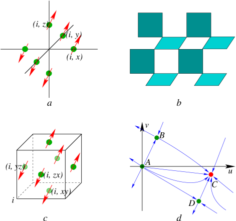
Figure 2: $(a)$, the lattice structure of the O($N$) spin-ice model. $(b)$, one of the plaquette configurations of CPM-2, with every site shared by two plaquettes. $(c)$, lattice structure for the O($N$) spin-plaquette model, each unit square face of the cubic lattice is occupied by an O($N$) vector, and the constraint is that the sum of all the O($N$) vectors on the twelve square faces shared by site $i$ is zero. $(d)$, the RG flow of Eq. 56 in the large-$N$ limit, $C$ is the stable fixed point, with enlarged $\mathrm{O}(N)\times\mathrm{O}(d)$ symmetry.

II.3 C, O($N$) Spin-Ice with Easy Plane Anisotropy

Model Eq. 11 is invariant under cubic lattice symmetry, and we can certainly turn on various anisotropies to this model, like what was studied in the CDM-1 model Chen et al. (2009). For instance, let us modify the model Eq. 11 slightly:

$$E = \sum_{i,\mu,a}J_{1,\mu}S^{a}_{i-\mu,\mu}S^{a}_{i,\mu}+\sum_{i,a}\sum_{\mu\neq\nu}J_{2,\mu\nu}S^{a}_{i,\mu}S^{a}_{i+\nu,\mu}.$$ (68)

If $J_{1,x}=J_{1,y}>J_{1,z}>0$, and $J_{2,xy}=J_{2,xz}=J_{2,yx}=J_{2,yz}>J_{2,zx}=J_{2,zy}>0$, the O($N$) spin vectors in the $xy$ plane, $S^{a}_{i,x}$ and $S^{a}_{i,y}$ have a stronger tendency to order compared with $S^{a}_{i,z}$. Therefore when we lower the temperature from the high temperature algebraic phase, the O($N$) vectors in $xy$ plane are expected to order first at critical temperature $T_{c1}$. In the field theory close to $T_{c1}$, the anisotropy can be described by an extra mass term for $\sum_{a}m^{2}(\phi^{a}_{z})^{2}$ in the free energy, which is clearly a relevant perturbation at the critical point $r=0$:

$$\mathcal{F} = \sum_{\mu,a}\phi^{a}_{\mu}(-\nabla^{2}+r)\phi^{a}_{\mu}+\sum_{a}m^{2}(\phi^{a}_{z})^{2}$$ (69)

$$+ \sum_{a}g(\sum_{\mu}\nabla_{\mu}\phi^{a}_{\mu})^{2}+\mathcal{F}_{4}.$$ (71)

In the equation above we have taken $\gamma=0$ for simplicity. To calculate the RG equations for $\mathcal{F}_{4}$, we still need to increase the dimension and flavor number to four with $\mu=x,\ y,\ z,\ \tau$, and the anisotropy of the generalized system will prefer the O($N$) vectors to order on three of the four axes. At the critical point $r=0$, due to the relevance of the extra mass term, we can safely take $m\rightarrow\infty$, and the correlation function between $\phi^{a}_{\mu}$ reads

$$\lim_{g,m\rightarrow\infty,r\rightarrow 0} D^{ab}_{\mu\nu}(\vec{q})=\langle\phi^{a}_{\mu}(\vec{q})\phi^{b}_{\nu}(-\vec{q})\rangle\sim\frac{\delta_{ab}}{q^{2}}Q_{\mu\nu},$$ (72)

$$Q_{\mu\nu} = \delta_{\mu\nu}-\frac{q_{\mu}q_{\nu}}{\mathrm{\mathbf{q}}^{2}},\ \mu,\nu\neq\tau,\ \mathrm{\mathbf{q}}^{2}=q_{x}^{2}+q_{y}^{2}+q_{\tau}^{2},$$ (74)

$$Q_{\mu\nu} = 0,\ \mu\ \mathrm{or}\ \nu=\tau.$$ (76)

Using the correlation function Eq. 76, the RG equation at the critical point reads

$$\frac{du}{d\ln l} = \epsilon u-8A(8+N)u^{2}-4N(A+B)v^{2}$$ (77)

$$- 4(A+B)w^{2}-4B(8+4N)uv$$ (79)

$$- 8(A+B)vw-48Buw,$$ (81)

$$\frac{dv}{d\ln l} = \epsilon v-16B(4+N)u^{2}-4(AN+3BN+4C)v^{2}$$ (83)

$$- 4Cw^{2}-16(2A+AN+BN+2B)uv$$ (85)

$$- 8(A+5B)vw-16(A+3B)uw,$$ (87)

$$\frac{dw}{d\ln l} = \epsilon w-64Bu^{2}-16Bv^{2}$$ (89)

$$- 4(A+6B+BN+2C+CN)w^{2}$$ (91)

$$- 16(B+2C)vw-32Auw,$$ (93)

$$\frac{dr}{d\ln l} = 2r-8(2A+AN+4B+2BN)ur$$ (95)

$$- 8(AN+2BN)vr-8(A+2B)wr.$$ (97)

Now $A=8/15$, $B=1/15$, $C=2/5$, which is different from the isotropic case, due to the different form of the correlation functions. Solving this equation at $r=0$, we again find a stable fixed point for large enough $N$. Expanded to the order of $\epsilon/N^{2}$, the stable fixed point is located at

$$u_{\ast} = \frac{27\epsilon}{112N}-\frac{1431\epsilon}{490N^{2}}+O(\frac{\epsilon}{N^{3}}),$$ (98)

$$\ v_{\ast} = -\frac{3\epsilon}{56N}-\frac{879\epsilon}{490N^{2}}+O(\frac{\epsilon}{N^{3}}),$$ (100)

$$w_{\ast} = \frac{15\epsilon}{28N}-\frac{1983\epsilon}{490N^{2}}+O(\frac{\epsilon}{N^{3}}),$$ (102)

Again, since $v_{\ast}+w_{\ast}=2u_{\ast}$, this fixed point has an enlarged $\mathrm{O}(N)\times\mathrm{O}(d-1)$ symmetry. Close to the stable fixed point, the three eigenvectors of the RG flow have scaling dimensions

$$\Delta_{1} = -\epsilon+O(\frac{\epsilon}{N^{2}}),$$ (103)

$$\Delta_{2} = -\epsilon+\frac{942\epsilon}{25N}+O(\frac{\epsilon}{N^{2}}),$$ (105)

$$\Delta_{3} = -\epsilon+\frac{1104\epsilon}{175N}+O(\frac{\epsilon}{N^{2}}).$$ (107)

$\Delta_{2}$ is the largest scaling dimension, and according to Eq. 97 the critical $N$ is $N_{c}\sim 59$, below which the stable fixed point disappears. Plug the fixed point value Eq. 102 back to the last RG equation in Eq. 97, we obtain the scaling dimension of $r$ at the fixed point:

$$[r]=\frac{1}{\nu}=2-\epsilon+\frac{138\epsilon}{7N}+O(\frac{\epsilon}{N^{2}}).$$ (108)

If we keep lowering the temperature after the order of $\phi^{a}_{x}$ and $\phi^{a}_{y}$, then eventually $\phi^{a}_{z}$ will also order at temperature $T_{c2}<T_{c1}$. After the order of $\phi^{a}_{x}$ and $\phi^{a}_{y}$, the O($N$) symmetry is broken down to its subgroup. Let us first assume $w<0$ in $\mathcal{F}_{4}$ $i.e.$ the three flavors of O($N$) vectors are collinear with each other in the low temperature ordered phase. Let us assume that in the intermediate phase the expectation value $\langle\phi^{a}_{x}\rangle\sim\langle\phi^{a}_{y}\rangle\sim(1,0,\cdots 0)$, now the O($N$) symmetry is broken down to O($N-1$) symmetry generated by Lie algebra $\Gamma_{ab}$ with $a,b=2,\cdots N$. This symmetry breaking implies that the degeneracy of the $N$ components of $\phi^{a}_{z}$ will be lifted at $T_{c2}$. Because $w<0$, the nonzero expectation value of $\phi^{1}_{x}$ and $\phi^{1}_{y}$ will prefer $\phi^{1}_{z}$ to order next at lower temperature, which is essentially an Ising transition with order parameter $\phi^{1}_{z}$. From now on we will denote $\phi^{1}_{z}$ as $\phi_{z}$. $\phi_{z}$ will couple to the gapped fluctuations $\phi_{x}=\phi^{1}_{x}-\langle\phi^{1}_{x}\rangle$ and $\phi_{y}=\phi^{1}_{y}-\langle\phi^{1}_{y}\rangle$ through the constraint, and the entire low energy field theory at $T_{c2}$ reads

$$\mathcal{F} = \phi_{z}(-\nabla^{2})\phi_{z}+\sum_{\mu=x,y}\phi_{\mu}(-\nabla^{2}+m^{2})\phi_{\mu}$$ (109)

$$+ g(\sum_{\mu}\nabla_{\mu}\phi_{\mu})^{2}+O(\phi_{z}^{4}).$$ (111)

After taking the limit $g\rightarrow\infty$, the critical correlation function of $\phi_{z}$ reads

$$\lim_{g\rightarrow\infty}D_{zz}(\vec{q})\sim\frac{1}{m^{2}\frac{q_{z}^{2}}{q_{x}^{2}+q_{y}^{2}}+q_{x}^{2}+q_{y}^{2}+\cdots}.$$ (112)

Therefore this transition at $T_{c2}$ is effectively a $z=2$ transition, with scaling dimension $[q_{z}]=2[q_{x}]=2[q_{y}]=2$. Now the total effective dimension is 4, and the $(\phi_{z})^{4}$ term is a marginally irrelevant perturbation, therefore this transition is a mean field transition with logarithmic corrections. Notice that the Goldstone modes after the O($N$) to O($N-1$) symmetry breaking are harmless to this transition. The Goldstone mode can be described by $\delta\phi^{a}_{x}\sim\delta\phi^{a}_{y}\sim(0,\pi^{2},\cdots\pi^{N})$ that forms a vector representation of O($N-1$), and in order to guarantee the gaplessness of the Goldstone modes, close to $T_{c2}$ the following coupling between $\phi_{z}$ and $\vec{\pi}$ is the lowest order coupling that is allowed:

$$\mathcal{F}_{goldstone}\sim\sum_{\mu}\phi_{z}^{2}(\nabla_{\mu}\vec{\pi})^{2}.$$ (113)

This term only generates irrelevant perturbations for $\phi_{z}$ at the transition. Couplings like $\phi_{z}^{2}(\vec{\pi})^{2}$ is forbidden due to its ability to renormalize the mass of Goldstone mode $\vec{\pi}$.

If $w>0$ in $\mathcal{F}_{4}$, then the three flavors of O($N$) vectors are perpendicular to each other in the low temperature ordered phase. Let us assume that in the intermediate phase between $T_{c1}$ and $T_{c2}$ the expectation values $\langle\phi^{a}_{x}\rangle\sim(1,0,\cdots 0)$ and $\langle\phi^{a}_{y}\rangle\sim(0,1,0\cdots 0)$. Now the O($N$) symmetry is broken down to the O($N-2$) symmetry generated by $\Gamma_{ab}$ with $a,b=3,\cdots N$. Due to the presence of $w$ term in $\mathcal{F}_{4}$, at $T_{c2}$ the order parameters should be $\phi^{a}_{z}$ with $a=3\cdots N$, which forms a vector representation of O($N-2$). In the intermediate phase there are in total $2N-3$ Goldstone modes, they are $\pi^{a}_{x}=(0,0,\pi^{3}_{x},\cdots\pi^{N}_{x})$ that corresponds to the O($N$) Lie algebra elements $\Gamma_{1a}$ with $a=3,\cdots N$; $\pi^{a}_{y}=(0,0,\pi^{3}_{y}\cdots\pi^{N}_{y})$ that correspond to the the O($N$) Lie algebra elements $\Gamma_{2a}$ with $a=3,\cdots N$; plus a rotation mode between $\phi^{1}_{x}$ and $\phi^{2}_{x}$, denoted as $\Gamma_{12}$. Again the order parameter $\phi^{a}_{z}$ will couple to these Goldstone modes through the constraint. The field theory close to $T_{c2}$ reads

$$\mathcal{F} = \sum_{\mu=x,y}\sum_{a=3}^{N}\pi^{a}_{\mu}(-\nabla^{2})\pi^{a}_{\mu}+\sum_{a=3}^{N}\phi^{a}_{z}(-\nabla^{2}+r)\phi^{a}_{z}$$ (114)

$$+ \sum_{a=3}^{N}g(\nabla_{z}\phi^{a}_{z}+\nabla_{x}\pi^{a}_{x}+\nabla_{y}\pi^{a}_{y})^{2}+O[(\phi_{z}^{a})^{4}].$$ (116)

Notice that the interaction between Goldstone modes $\pi^{a}_{\mu}$ have to be irrelevant to guarantee their gaplessness. The universality class of this transition at $r=0$ can be calculated using the correlation function of $\phi^{a}_{z}$ after taking the limit $g\rightarrow\infty$:

$$\lim_{g\rightarrow\infty,r\rightarrow 0}D^{ab}_{zz}(\vec{q})\sim\frac{(q_{x}^{2}+q_{y}^{2})}{(q_{x}^{2}+q_{y}^{2}+q_{z}^{2})^{2}}\delta_{ab}.$$ (117)

The first order $\epsilon$ expansion leads to the following scaling dimension and critical exponent:

$$[r]=\frac{1}{\nu}=2-\frac{N-1}{N+5}\epsilon,$$ (118)

which is identical to the 3d O($N-2$) Wilson-Fisher (WF) fixed point, although higher order expansions may deviate from the WF fixed point. Therefore our formalism implies that with large enough $N$, the easy plane anisotropy will split the transition discussed in the previous subsection to two second order transitions.

II.4 D, O($N$) Spin-Ice with Easy Axis Anisotropy

In model Eq. 68, if we make the following choice of parameters: $J_{1,z}>J_{1,x}=J_{1,y}>0$, $J_{2,zx}=J_{2,zy}>J_{2,xy}=J_{2,xz}=J_{2,yx}=J_{2,yz}$, then when we lower the temperature from the algebraic phase, the O($N$) vectors along the $z$ axis will order first at temperature $T_{c1}$. Similar to the previous section, this easy axis anisotropy can be described by an extra mass gap $m$ for both $\phi^{a}_{x}$ and $\phi^{b}_{y}$ modes in the field theory Eq. 20, and $\phi^{a}_{z}$ becomes the only order parameter at low energy. However, now we can no longer take the limit $m\rightarrow\infty$, because with this limit all the correlation functions will vanish. If we keep $m$ finite, the correlation function of $\phi^{a}_{z}$ takes a similar form as Eq. 112:

$$\lim_{g\rightarrow\infty}D^{ab}_{zz}(\vec{q})\sim\frac{\delta_{ab}}{m^{2}\frac{q_{z}^{2}}{q_{x}^{2}+q_{y}^{2}}+q_{x}^{2}+q_{y}^{2}+\cdots},$$ (119)

therefore this transition is again an effective a $z=2$ mean field transition. A similar situation with easy axis anisotropy has been studied in Ref. Pickles et al. (2008), although there the easy axis was along the diagonal direction.

If the temperature is lowered even more from $T_{c1}$, then at $T_{c2}$ the spin vectors within $xy$ planes will order next. Again the nature of this transition would depend on the sign of $w$ in $\mathcal{F}_{4}$. If $w<0$ $i.e.$ the three flavors of O($N$) vectors order collinearly, then if $\phi^{a}_{z}$ orders along direction $\langle\phi^{a}_{z}\rangle\sim(1,0\cdots 0)$, at temperature $T_{c2}$ $\phi^{1}_{x}$ and $\phi^{1}_{y}$ will become the critical modes. $\phi^{1}_{x}$ and $\phi^{1}_{y}$ are coupled to the gapped fluctuation $\phi_{z}=\phi^{1}_{z}-\langle\phi^{1}_{z}\rangle$, and the low energy field theory describing $\phi_{x}$ and $\phi_{y}$ is identical to Eq. 71 with $N=1$. By solving the RG equation Eq. 97 with $N=1$, no stable fixed point is found.

If $w>0$, the critical modes at $T_{c2}$ is $\phi^{a}_{x}$ and $\phi^{a}_{y}$ with $a=2,\cdots N$, which form vector representations of O($N-1$). These two critical modes are coupled to gapless Goldstone mode $\pi^{a}_{z}=(0,\pi^{2}_{z},\cdots\pi^{N}_{z})$, with field theory

$$\mathcal{F} = \sum_{\mu=x,y}\sum_{a=2}^{N}\phi^{a}_{\mu}(-\nabla^{2}+r)\phi^{a}_{\mu}+\sum_{a=2}^{N}K\pi^{a}_{z}(-\nabla^{2})\pi^{a}_{z}$$ (120)

$$+ \sum_{a=3}^{N}g(\nabla_{z}\pi^{a}_{z}+\nabla_{x}\phi^{a}_{x}+\nabla_{y}\phi^{a}_{y})^{2}+\mathcal{F}_{4}(\phi^{a}_{x},\phi_{y}^{a}).$$ (122)

Now $\mathcal{F}_{4}$ only involves two flavors of O($N-1$) vectors $\phi^{a}_{x}$ and $\phi^{a}_{y}$. Number $K$ is in general not 1 because the now there is no symmetry that can transform $\phi^{a}_{x}$, $\phi^{a}_{y}$ and $\pi^{a}_{z}$. Again, the renormalization of $K$ will be an order $\epsilon^{2}$ effect, therefore we can take $K$ as a constant. The RG equation for $\mathcal{F}_{4}$ can be calculated in the same manner as we did before. If we take $K=1$, then the RG equation for $\mathcal{F}_{4}$ takes the same form as Eq. 97 but with $A=5/8$, $B=1/24$, $C=13/24$. With large enough $N$ there is still a stable fixed point, and the answer is qualitatively unchanged when $K$ deviates from 1 slightly.

III III, O($N$) Spin-Plaquette Model

III.1 A, Phase Transition with General $N$

Now we switch the gear to the less well studied spin-plaquette model, where the physical quantities are defined on the unit square faces of the cubic lattice instead of the links. In Ref. Xu and Wu (2008); Pankov et al. (2007), a model of this type was studied, with every site of the cubic lattice connects to precisely one filled plaquette. Physically the filled plaquette is a SU(4) singlet formed with four SU(4) fundamental fermions on four corners of the plaquette. This model is denoted as CPM-1. In this section we will study an O($N$) generalization of this model. We define an O($N$) spin vector $S^{a}_{i,\mu\nu}$ on each unit face of the cubic lattice, and impose the constraint

$$\sum_{\mu,\nu=x,y,z}S^{a}_{i,\mu\nu}+S^{a}_{i-\mu,\mu\nu}+S^{a}_{i-\nu,\mu\nu}+S^{a}_{i-\mu-\nu,\mu\nu}=0.$$ (123)

In addition to this constraint, we consider the following Hamiltonian:

$$E=\sum_{i,\mu,\nu}J_{1}S^{a}_{i,\mu\nu}S^{a}_{i+\mu,\mu\nu}+J_{2}S^{a}_{i,\mu\nu}S^{a}_{i+\rho,\mu\nu},\rho\neq\mu,\nu.$$ (124)

When $J_{1}>0$, $J_{2}>0$, the ground state of this Hamiltonian has staggered order with nonzero $\langle\phi^{a}_{i,\mu\nu}\rangle\sim(-1)^{i}S^{a}_{i,\mu\nu}$ with $\mu,\nu=+x,+y,+z$. $\phi^{a}_{\mu\nu}$ is a symmetric tensor with $\mu\neq\nu$, which has only three independent flavors. Under discrete cubic lattice symmetry, tensor field $\phi^{a}_{\mu\nu}$ transforms as

$$T_{\mu} : \ i\rightarrow i+\mu,\ \phi^{a}_{\nu\rho}\rightarrow-\phi^{a}_{\nu\rho},\ (\mathrm{for}\ \mathrm{all}\ \mu,\ \nu,\ \rho),$$ (125)

$$R_{\mu,s} : \ \mu\rightarrow-\mu,\ \phi^{a}_{\mu\nu}\rightarrow-\phi^{a}_{\mu\nu},\ \phi^{a}_{\nu\rho}\rightarrow\phi^{a}_{\nu\rho},\ (\mathrm{for}\ \nu,\rho\neq\mu),$$ (127)

$$R_{\mu\nu} : \ \mu\leftrightarrow\nu,\ \phi^{a}_{\mu\rho}\leftrightarrow\phi^{a}_{\nu\rho},\ (\mathrm{for}\ \nu\neq\mu).$$ (129)

Just like the spin-ice model Eq. 11, the ground state of model Eq. 124 also has enlarged symmetry $[\mathrm{O}(N)]^{3}$ $i.e.$ the spins on different planes will order independently. Since $\phi^{a}_{\mu\nu}$ is subject to the constraint Eq. 6, we can start with the following low energy field theory close to the transition:

$$\mathcal{F} = \sum_{\mu\neq\nu,a}\phi^{a}_{\mu\nu}(-\nabla^{2}+r)\phi^{a}_{\mu\nu}+\sum_{a}g(\sum_{\mu,\nu}\nabla_{\mu}\nabla_{\nu}\phi^{a}_{\mu\nu})^{2}$$ (130)

$$+ \mathcal{F}_{4},$$ (132)

and $\mathcal{F}_{4}$ is all the quartic terms allowed by symmetry:

$$\mathcal{F}_{4} = u\sum_{\mu<\nu}[\sum_{a}(\phi^{a}_{\mu\nu})^{2}]^{2}+v\sum_{\nu<\rho}[\sum_{a}(\phi^{a}_{\mu\nu})^{2}][\sum_{b}(\phi^{b}_{\mu\rho})^{2}]$$ (133)

$$+ w\sum_{\nu\neq\rho}[\sum_{a}\phi^{a}_{\mu\nu}\phi^{a}_{\mu\rho}][\sum_{b}\phi^{b}_{\mu\nu}\phi^{b}_{\mu\rho}].$$ (135)

Under the limit $g\rightarrow\infty$, the constraint Eq. 6 is effectively imposed, and the correlation function with $r>0$ is:

$$\lim_{g\rightarrow\infty}D^{ab}_{\mu\nu,\rho\sigma} = \langle\phi^{a}_{\mu\nu}(\vec{q})\phi^{b}_{\rho\sigma}(-\vec{q})\rangle\sim\frac{\delta_{ab}}{r+q^{2}}R_{\mu\nu\rho\sigma},$$ (136)

$$R_{\mu\nu\rho\sigma} = (\delta_{\mu\rho}\delta_{\nu\sigma}+\delta_{\mu\sigma}\delta_{\nu\rho}$$ (138)

$$- \frac{q_{\mu}q_{\nu}q_{\rho}q_{\sigma}}{q_{x}^{2}q_{y}^{2}+q_{y}^{2}q_{z}^{2}+q_{x}^{2}q_{z}^{2}}).$$ (140)

Notice that in Eq. 132, some extra flavor-orbital coupling quadratic terms are allowed by symmetry, such as

$$\mathcal{F}_{2}\sim\sum_{a}\nabla_{x}\phi^{a}_{yz}\nabla_{y}\phi^{a}_{xz}+\nabla_{y}\phi^{a}_{zx}\nabla_{z}\phi^{a}_{xy}+\nabla_{z}\phi^{a}_{xy}\nabla_{x}\phi^{a}_{yz}.$$ (141)

Just like the $\gamma$ term in Eq. 20, this term will not gain any renormalization at the one-loop calculation $i.e.$ its RG flow will only affect the RG equation of $u$, $v$ and $w$ at the order of $\epsilon^{3}$. A small perturbation of this term will not change the RG flow qualitatively, we will take this term to be zero hereafter for simplicity.

To calculate the RG equation at the critical point $r=0$, in principle we need to generalize the model to 4d. However, there is no ideal way to make this generalization. For instance, if we define O($N$) vectors on the 2d faces of a 4d lattice, and $\mu$ takes $x,\ y,\ z,\ \tau$, at 4d there are two extra quartic terms in addition to $\mathcal{F}_{4}$ in Eq. 135:

$$\mathcal{F}_{4a} \sim [\sum_{a}\phi^{a}_{xy}\phi^{a}_{yz}][\sum_{b}\phi^{b}_{z\tau}\phi^{b}_{\tau x}]+\cdots$$ (142)

$$\mathcal{F}_{4b} \sim [\sum_{a}\phi^{a}_{xy}\phi^{a}_{z\tau}][\sum_{b}\phi^{b}_{yz}\phi^{b}_{\tau x}]+\cdots$$ (144)

These two extra terms will make the RG equation much more complicated than the actual 3d case. For instance, since these two terms are allowed by symmetry, they will be generated under RG flows even if we take them to be zero at the beginning. Therefore in this section we will just evaluate the loop integrals at 3d.

The RG equation takes exactly the same form as Eq. 97, while now $A=5/9$, $B=1/18$, $C=7/18$. With large enough $N$, there is a stable fixed point located at

$$u_{\ast} = \frac{11\epsilon}{48N}-\frac{29579\epsilon}{10368N^{2}}+O(\frac{\epsilon}{N^{3}}),$$ (145)

$$\ v_{\ast} = -\frac{\epsilon}{24N}-\frac{19039\epsilon}{10368N^{2}}+O(\frac{\epsilon}{N^{3}}),$$ (147)

$$w_{\ast} = \frac{9\epsilon}{16N}-\frac{22171\epsilon}{5184N^{2}}+O(\frac{\epsilon}{N^{3}}),$$ (149)

Close to the stable fixed point, the three eigenvectors of the RG flow have scaling dimensions

$$\Delta_{1} = -\epsilon+O(\frac{\epsilon}{N^{2}}),$$ (150)

$$\Delta_{2} = -\epsilon+\frac{6.80\epsilon}{N}+O(\frac{\epsilon}{N^{2}}),$$ (152)

$$\Delta_{3} = -\epsilon+\frac{37.5\epsilon}{N}+O(\frac{\epsilon}{N^{2}}).$$ (154)

Plug the fixed point value Eq. 102 back to the last RG equation in Eq. 97, we obtain the scaling dimension of $r$ at the fixed point:

$$[r]=\frac{1}{\nu}=2-\epsilon+\frac{2113\epsilon}{108N}+O(\frac{\epsilon}{N^{2}})$$ (155)

If $N=1$, no stable fixed point is found. The case $N=1$ is equivalent to CPM-6, which is much less studied compared with the CDM-$m$. We will discuss this model in the next subsection.

III.2 B, Duality and $N=1$

Besides taking the limit $g\rightarrow\infty$ in the Gaussian field theory Eq. 132, the correlation function in Eq. 140 can be obtained by other means. Let us solve the constraint Eq. 6 with softened unit length constraint of $\phi^{a}_{\mu\nu}$ by defining the three flavors of O($N$) height field $h^{a}_{\mu}$ on the cubic center $\bar{i}$ of the lattice:

$$\phi^{a}_{xy} = \nabla_{z}(h^{a}_{x}-h^{a}_{y}),$$ (156)

$$\phi^{a}_{zy} = \nabla_{x}(h^{a}_{z}-h^{a}_{y}),$$ (158)

$$\phi^{a}_{zx} = \nabla_{y}(h^{a}_{z}-h^{a}_{x}).$$ (160)

Then height field $h^{a}_{\mu}$ plays the same role as vector potential $A_{\mu}$ in the usual dimer model. Now in terms of the height field, the algebraic phase can be described by the following Gaussian field theory

$$\mathcal{F} = \sum_{a}\frac{K}{2}[\nabla_{z}(h^{a}_{x}-h^{a}_{y})]^{2}+[\nabla_{y}(h^{a}_{z}-h^{a}_{x})]^{2}$$ (161)

$$+ [\nabla_{x}(h^{a}_{y}-h^{a}_{z})]^{2}+\cdots$$ (163)

This Gaussian field theory takes a similar form as the Khaliullin model describing the orbital degrees of freedom Khaliullin and Maekawa (2000), after taking the spin-wave expansion. Diagonalizing this Gaussian field theory, we obtain two eigenmodes describing the fluctuations of the height vector field:

$$\omega_{1}^{2}\sim\frac{q_{x}^{2}q_{y}^{2}+q_{y}^{2}q_{z}^{2}+q_{z}^{2}q_{x}^{2}}{q^{2}},\ \ \ \omega_{2}^{2}\sim q^{2}.$$ (164)

Interestingly $\omega_{1}$ vanishes along each coordinate axis in the momentum space. This height field theory Eq. 163 is invariant under the following symmetry transformation:

$$h^{a}_{x}\rightarrow h^{a}_{x}+f_{1}(x)+\varphi(x,y,z),$$ (165)

(166)

$$h^{a}_{y}\rightarrow h^{a}_{y}+f_{2}(y)+\varphi(x,y,z),$$ (167)

(168)

$$h^{a}_{z}\rightarrow h^{a}_{z}+f_{3}(z)+\varphi(x,y,z).$$ (169)

$f_{\alpha}$ are functions of only one of the coordinates, this type of quasi-local symmetry comes from the definition of the height field Eq. 160, and hence does not depend on the detailed form of the Hamiltonian. This quasi-local symmetry is responsible for the line of nodes of the eigenmodes in Eq. 164. Using the Gaussian free energy, and the height representation of $\phi^{a}_{\mu\nu}$ in Eq. 160, we can reproduce the correlation function Eq. 140.

These dualities are particularly useful for $N=1$, which is equivalent to CPM-6. Since in this case $\phi_{\mu\nu}$ takes discrete values, then $h_{\mu}$ are also discrete. Therefore in the dual field theory Eq. 163 for $N=1$ we should also consider the vertex operators like we introduced for the CDM, in section II-A. For convenience, let us make the following standard modification of our description of the system: we will allow $\phi_{\mu\nu}$ to take all the half-integer values, and turn on classical Hamiltonian on the lattice $E=\sum_{i,\mu\neq\nu}U(\phi_{i,\mu\nu})^{2}$, on top of the constraint $\sum_{\mu\neq\nu}\nabla_{\mu}\nabla_{\nu}\phi_{\mu\nu}=0$. When $U$ is large, effectively on every unit face $\phi_{i,\mu\nu}$ can only take two values, which is the same as the CPM-6. In this way, even though we increased the total configurations of $\phi_{\mu\nu}$, the low energy configurations of $\phi_{\mu\nu}$ is still identical to the CPM-6. Now the dual field theory of the algebraic phase reads

$$\mathcal{F} = \frac{K}{2}[\nabla_{z}(h_{x}-h_{y})]^{2}+[\nabla_{y}(h_{z}-h_{x})]^{2}$$ (170)

$$+ [\nabla_{x}(h_{y}-h_{z})]^{2}.$$ (172)

In order to make sure $\phi_{\mu\nu}$ take half-integer values, based on the definite Eq. 160, $h_{\mu}-h_{\nu}$ will take site-dependent integer or half-integer values on the 3d dual cubic lattice:

$$h_{x}-h_{y} \in \mathbb{Z}+\frac{1-(-1)^{\bar{i}_{z}+\bar{i}_{x}}}{4},$$ (173)

$$h_{y}-h_{z} \in \mathbb{Z}+\frac{1-(-1)^{\bar{i}_{x}+\bar{i}_{y}}}{4},$$ (175)

$$h_{z}-h_{x} \in \mathbb{Z}+\frac{1-(-1)^{\bar{i}_{y}+\bar{i}_{z}}}{4}.$$ (177)

Then in the dual theory the lowest order vertex operator that do not have spatial oscillation is

$$\mathcal{F}_{v}=\sum_{\mu\neq\nu}-\alpha\cos[4\pi(h_{\mu}-h_{\nu})].$$ (178)

It was shown in Ref. Xu and Wu (2008) that this vertex operator has directional dependent algebraic correlation in the algebraic phase, with scaling dimension proportional to $K$ in Eq. 172. For instance, let us denote $\cos[4\pi(h_{x}-h_{y})]$ as $\mathcal{F}_{v,xy}$, then due to the quasi-local symmetry in Eq. 169, two $\mathcal{F}_{v,xy}$ operators can only have nonzero correlation when they are on the same $z$ axis:

$$\langle\mathcal{F}_{v,xy}(0,0,0)\mathcal{F}_{v,xy}(0,0,z)\rangle$$ (179)

$$\sim \exp\{-\frac{4(2\pi)^{2}}{K}\int\frac{d^{3}k}{(2\pi)^{3}}\frac{(k_{x}^{2}+k_{y}^{2})e^{ik_{z}z}}{k_{x}^{2}k_{y}^{2}+k_{y}^{2}k_{z}^{2}+k_{x}^{2}k_{z}^{2}}\}$$ (181)

$$\sim \frac{1}{z^{16\pi/K}}.$$ (183)

If the scaling dimension $8\pi/K$ is greater than 1 $i.e.$ $K>K_{c1}=8\pi$, the vertex operator Eq. 178 becomes relevant in the algebraic phase. The relevance of this vertex operator can be manifested by directly calculating the partition function with expansion of the vertex operator. The second order perturbation involves the integral of the correlation function Eq. 183, and if $K>K_{c1}$, the integral diverges in the infrared limit.

the proliferation of the vertex operator will drive a Kosterlitz-Thouless (KT) transition, across which the algebraic correlation disappears, and the correlation length of the vertex operators diverges as $\xi\sim\exp[\sqrt{\frac{c}{K-K_{c1}}}]$. This KT transition in 3d space is due to the special quasilocal symmetry in Eq. 169, which grants the 3d system a 2d like symmetry for each flavor of $h_{\mu}$. The KT transition and dimensional reduction behavior in 3d or 2+1d were also discussed in another type of U(1) rotor systems with similar quasilocal symmetries Paramekanti et al. (2002); Balents and Fisher (2005); Xu and Moore (2005). What is different here is that, this dimensional reduction behavior in our system is inherited from the generic quasi-local symmetry in the definition of height field Eq. 160, therefore dimensional reduction is robust.

There is another useful duality of Eq. 163. Consider the following Gaussian field theory:

$$\mathcal{F}=\sum_{a=1}^{N}\frac{1}{2K}[(\nabla_{x}\nabla_{y}\theta^{a})^{2}+(\nabla_{y}\nabla_{z}\theta^{a})^{2}+(\nabla_{z}\nabla_{x}\theta^{a})^{2}],$$ (184)

Now let us introduce the new field $\phi^{a}_{\mu\nu}$ through Hubbard-Stratonovich transformation:

$$\mathcal{F}=\sum_{\mu\neq\nu,a}\frac{K}{2}(\phi^{a}_{\mu\nu})^{2}-i\phi^{a}_{\mu\nu}\nabla_{\mu}\nabla_{\nu}\theta^{a}.$$ (185)

After integrating out the field $\theta^{a}$, the partition function of the system becomes

$$Z=\int D\phi^{a}_{\mu\nu}\delta(\sum_{\mu\neq\nu}\nabla_{\mu}\nabla_{\nu}\phi^{a}_{\mu\nu})e^{-\int d^{3}x\sum_{a}\sum_{\mu\neq\nu}\frac{K}{2}(\phi^{a}_{\mu\nu})^{2}}.$$ (186)

The delta function in this partition imposes the same constraint Eq. 6. The field theory Eq. 184 is also invariant under quasi-local symmetry transformation:

$$\theta^{a}\rightarrow\theta^{a}+g^{a}_{1}(x)+g^{a}_{2}(y)+g^{a}_{3}(z).$$ (187)

$g^{a}_{\alpha}$ are arbitrary functions of one of the three coordinates. The field theories Eq. 184 and Eq. 163 are dual to each other, with the same parameter $K$.

IV IV, Defects of Constraints

IV.1 A, Affects on the Algebraic Phase

So far all the constraints have been perfectly imposed, and in this section we will consider the case with slightly softened constraint son $i.e.$ we allow the existence of the point defect that violates the constraint. In the algebraic phase, for all the O($N$) models considered in this work, if $g$ is large but finite in Eq. 20, 71, 132, the power-law correlation immediately crossovers back to short range correlation for large enough distance. For instance, take the correlation function Eq. 24, we can see that the length scale for this crossover is $l\sim\sqrt{g/r}$ for O($N$) spin-ice.

The Gaussian theory evaluation of the defects is based on the assumption that the defect can take continuous values, therefore the “charge” of the defect $\sum_{\mu}\nabla_{\mu}\phi^{a}_{\mu}$ can be infinitesimal. Therefore the Gaussian theory is no longer applicable for $N=1$, where the defect charge is always discrete. To evaluate the defect in this case, one needs to go to the other side of the duality. For instance, the CDM-$m$ is dual to the Villain form of U(1) rotor model with partition function

$$Z=\int D\theta\sum_{l_{i,\mu}}\exp[ - \sum_{i,\mu}\frac{1}{2\tilde{K}}(\theta_{i}-\theta_{i+\mu}-2\pi l_{i,\mu})^{2}$$ (188)

$$+ 2\pi i\frac{m}{6}l_{i,\mu}(-1)^{i}].$$ (190)

Notice that there is an imaginary term in the partition function due to the nonzero average filling of the dimer density, which is similar to the Berry phase of quantum Bose rotor model with fractional boson filling Powell and Chalker (2009). To show this duality explicitly, we still introduce the field $\phi_{i,\mu}$ through Hubbard-Stratonovich transformation

$$Z = \int D\theta D\phi_{i,\mu}\sum_{l_{i,\mu}}\exp[\sum_{i,\mu}-\frac{\tilde{K}}{2}\phi^{2}_{i,\mu}-i\nabla_{\mu}\phi_{i,\mu}\theta_{i}$$ (191)

$$- 2\pi il_{i,\mu}(\phi_{i,\mu}+(-1)^{i}\frac{m}{6})].$$ (193)

After integrating out the $\theta_{i}$, and summing over $l_{i,\mu}$, the dual theory reads

$$Z=\sum_{\phi_{\mu}}\delta(\sum_{\mu}\nabla_{\mu}\phi_{\mu})\exp[\sum_{i,\mu}-\frac{\tilde{K}}{2}(\phi_{i,\mu})^{2}],$$ (194)

and $(-1)^{i}\phi_{i,\mu}\in\mathbb{Z}+m/6$. Then any low energy configuration of $\phi_{i,\mu}$ is equivalent to a CDM-$m$ configuration.

If we are in the superfluid phase of the rotor model, which is dual to the algebraic phase of the CDM-$m$, we can expand the free energy of the rotor model Eq. 184 at $l_{i,\mu}=0$, and the field theory of the superfluid phase is simply $\mathcal{F}=\frac{1}{2K}(\nabla_{\mu}\theta)^{2}$. The defects will be taken into account by the vertex operator in the field theory:

$$\mathcal{F}=\sum_{\mu}\frac{1}{2K}(\nabla_{\mu}\theta)^{2}-\alpha\cos(\theta),$$ (195)

$\alpha\sim\exp(-\mathcal{C}_{1}g)$ is the fugacity of the defect, and the partition function with expansion of $\alpha$ is equivalent to a classical Coulomb gas, which is equivalent to the partition function of defects. In 3d space since $\theta$ has long range order, $\alpha$ is a very relevant perturbation $i.e.$ the presence of defects will immediately destroy the algebraic phase with infinitesimal fugacity. Another way to show the relevance of the defect is to compare the energy and entropy of an isolated defect. If the system size is $L^{3}$, then an isolated defect in the algebraic phase costs energy $E\sim\int d^{3}k\frac{1}{k^{2}}\sim g\mathcal{A}+\frac{1}{L}$ which is finite in the infrared limit. While the entropy of the defect scales as $S\sim\ln L$, therefore the entropy always dominates energy $i.e.$ the defects always proliferate.

The situation is very different for the CPM-$m$. Just like the duality of the CDM-$m$, the CPM-$m$ is dual to the following rotor model:

$$Z=\int D\theta\sum_{l_{i,\mu\nu}}\exp[ - \sum_{i,\mu\neq\nu}\frac{1}{2\tilde{K}}(\nabla_{\mu\nu}\theta-2\pi l_{i,\mu\nu})^{2}$$ (196)

$$+ 2\pi i\frac{m}{12}l_{i,\mu\nu}(-1)^{i}].$$ (198)

Again, in the algebraic phase of the CPM-$m$, we can expand the free energy at $l_{i,\mu\nu}=0$, and evaluate the relevance of defects in the rotor field theory:

$$\mathcal{F}=\sum_{\mu\neq\nu}\frac{1}{2K}(\nabla_{\mu}\nabla_{\nu}\theta)^{2}-\alpha\cos(\theta).$$ (199)

Now because of the quasi-local symmetry Eq. 187, the vertex operator $\mathcal{F}_{v}=-\alpha\cos(\theta)$ has no nonzero correlation spatially, which seemingly implies that the defect is irrelevant. This effect can again be shown by evaluating the energy and entropy of the defect. An isolated defect costs energy

$$E\sim\int d^{3}k\frac{1}{k_{x}^{2}k_{y}^{2}+k_{y}^{2}k_{z}^{2}+k_{z}^{2}k_{x}^{2}}\sim L+c\ln L,$$ (200)

which always dominates the entropy that scales as $\ln L$ $i.e.$ the defects are always suppressed by energy.

However, although nonzero correlation between $\mathcal{F}_{v}$ is forbidden by symmetry, the correlation between defect-dipole operator $\mathcal{F}_{d,\mu}\sim-\alpha^{\prime}\cos(\nabla_{\mu}\theta)=-\alpha^{\prime}\cos(\theta_{i}-\theta_{i+\mu})$ can be nonzero. For instance, $\mathcal{F}_{d,z}$ can have nonzero correlation within the entire $xy$ plane:

$$\langle\mathcal{F}_{d,z}(0,0,0)\mathcal{F}_{d,z}(x,y,0)\rangle$$ (201)

$$\sim \exp\{-K\int\frac{d^{3}k}{(2\pi)^{3}}\frac{k_{z}^{2}e^{ik_{x}x+ik_{y}y}}{k_{x}^{2}k_{y}^{2}+k_{y}^{2}k_{z}^{2}+k_{x}^{2}k_{z}^{2}}\}$$ (203)

$$\sim \frac{1}{(x^{2}+y^{2})^{K/(4\pi)}}.$$ (205)

When $K<K_{c2}=8\pi$, the vertex dipole operator $\mathcal{F}_{d,\mu}$ is relevant, and the algebraic phase disappears. Suppose $\alpha^{\prime}\sim\alpha^{2}\sim\exp(-\mathcal{C}_{2}g)$ is the fugacity of the defect dipole, the crossover length scale beyond which the dipole becomes important is $\xi\sim(\alpha^{\prime})^{4\pi/(K_{c2}-K)}$. Again we can compare the energy of a defect dipole and its entropy. The energy of a defect dipole scales as $E\sim\int d^{3}kk_{z}^{2}/(k_{x}^{2}k_{y}^{2}+k_{y}^{2}k_{z}^{2}+k_{z}^{2}k_{x}^{2})\sim\ln L$, which is comparable with the entropy. So by tuning $K$ in Eq. 199, there will be a KT transition as a result of the competition between entropy and energy.

IV.2 B, Effects on the Transition

Close to the transition $r=0$, we can use the correlation function Eq. 24 to compute the RG equation. $g$ may flow under RG eventually, but it remains a constant at the first order $\epsilon$ expansion, and hence we will just take it a constant. For the isotropic O($N$) spin-ice, the RG equation takes the same form as Eq. 56, but now we need to reevaluate the loop integrals:

$$A = \frac{5}{8}+\frac{1}{8(1+g)^{2}}+\frac{1}{4(1+g)},$$ (206)

$$B = \frac{g^{2}}{24(1+g)^{2}},$$ (208)

$$C = \frac{13}{24}+\frac{1}{24(1+g)^{2}}+\frac{5}{12(1+g)}.$$ (210)

Solve the equation Eq. 56 with the new parameters Eq. 210, we can see that when $g$ is large, the solutions are qualitatively unchanged from Eq. 102. While when $g<g_{c}\sim 4.1$, stable fixed points are found with $N=1$, which corresponds to CDM-3 with softened constraint. For instance, with $N=1$, $g=1$, the stable fixed point is located at $u_{\ast}=\frac{53-\sqrt{37}}{3330}$, $v_{\ast}+w_{\ast}=\frac{7+\sqrt{37}}{555}$. Now in the low temperature phase the connected correlation on top of the long range order is also short-ranged after the transition described above.

With finite $g$, the O($N$) spin-ice with easy-plane axis can be studied in a similar way as last paragraph. As was mentioned in section II. A, we need to generalize the system to 4d with $\mu=x,\ y,\ z,\ \tau$, and anisotropy of the Hamiltonian prefers the O($N$) spin vectors on $x,\ y,\ z$ axes to order first at $T_{c1}$. At the critical point $T_{c1}$ with $r=0$, the 4d correlation function between $\phi^{a}_{\mu}$ reads

$$\lim_{m\rightarrow\infty,r\rightarrow 0}D^{ab}_{\mu\nu} \sim \frac{\delta_{ab}}{q^{2}}(\delta_{\mu\nu}-\frac{gq_{\mu}q_{\nu}}{q_{\tau}^{2}+(1+g)\mathbf{q}^{2}})\ ,\mu,\nu\neq\tau,$$ (211)

$$\mathrm{\mathbf{q}}^{2} = q_{x}^{2}+q_{y}^{2}+q_{\tau}^{2},$$ (213)

$$\lim_{m\rightarrow\infty,r\rightarrow 0}D^{ab}_{\mu\nu} = 0,\ \mu\ \mathrm{or}\ \nu=0.$$ (215)

The RG equation in this case takes the same form as Eq. 97, with different $A$, $B$ and $C$. Expanded to the first order of $1/g$, these parameters read:

$$A = \frac{8}{15}+\frac{8}{15g}+O(\frac{1}{g^{2}}),$$ (216)

$$B = \frac{1}{15}-\frac{4}{15g}+O(\frac{1}{g^{2}}),$$ (218)

$$C = \frac{2}{5}+\frac{16}{15g}+O(\frac{1}{g^{2}}).$$ (220)

When $g<g_{c}\sim 4.4$, stable fixed points are found with $N=1$, which corresponds to CDM-3 with softened constraint and easy plane anisotropy. With easy-axis anisotropy and finite $g$, the effective $z=2$ physics in Eq. 119 is absent, and the universality class is expected to crossover back to a 3d Wilson-Fisher transition.

In the O($N$) spin-plaquette model, since the $g$ term has higher derivatives compared with the Gaussian part of the field theory Eq. 132, then $g$ becomes irrelevant when its initial value is finite. Since at the low energy effective field theory, there is no flavor-orbital mixing interaction, we can take a more concise notation: $\phi^{a}_{x}=\phi^{a}_{yz}$, $\phi^{a}_{y}=\phi^{a}_{zx}$, $\phi^{a}_{z}=\phi^{a}_{xy}$. At the critical point $r=0$ the O($N$) spin-plaquette model is described by the field theory:

$$\mathcal{F}=\sum_{\mu,a}-\phi^{a}_{\mu}\nabla^{2}\phi^{a}_{\mu}+\mathcal{F}_{4},$$ (221)

with $\mathcal{F}_{4}$ given by Eq. 23. Now the coupled RG equation for $u$, $v$ and $w$ reads

$$\frac{du}{d\ln l} = \epsilon u-8(8+N)u^{2}-4Nv^{2}-4w^{2}-8vw,$$ (222)

$$\frac{dv}{d\ln l} = \epsilon v-4(4+N)v^{2}-4w^{2}$$ (224)

$$- 16(2+N)uv-24vw-16uw,$$ (226)

$$\frac{dw}{d\ln l} = \epsilon w-4(3+N)w^{2}-16vw-32uw,$$ (228)

$$\frac{dr}{d\ln l} = 2r-8(2+N)ur-8Nvr-8wr.$$ (230)

For large enough $N$, there are in total eight fixed points. For instance, the fixed point $w_{\ast}=0$, $v_{\ast}=2u_{\ast}=\epsilon/(12N)+\cdots$ has enlarged O(3$N$) symmetry, which mixes the flavor and spin symmetry. Expanded to the order of $\epsilon/N^{2}$, the only stable fixed point with $r=0$ is located at

$$u_{\ast} = \frac{\epsilon}{8N}-\frac{5\epsilon}{4N^{2}}+O(\frac{\epsilon}{N^{2}}),$$ (231)

$$\ v_{\ast} = -\frac{3\epsilon}{4N^{2}}+O(\frac{\epsilon}{N^{2}}),$$ (233)

$$\ w_{\ast} = \frac{\epsilon}{4N}-\frac{7\epsilon}{4N^{2}}+O(\frac{\epsilon}{N^{2}}).$$ (235)

Close to the stable fixed points, the three eigenvectors of the RG flow have scaling dimensions

$$\Delta_{1} = -\epsilon+O(\frac{\epsilon}{N^{2}}),$$ (236)

$$\Delta_{2} = -\epsilon+\frac{4\epsilon}{N}+O(\frac{\epsilon}{N^{2}}),$$ (238)

$$\Delta_{3} = -\epsilon+\frac{20\epsilon}{N}+O(\frac{\epsilon}{N^{2}}).$$ (240)

The scaling dimension of $r$ at this fixed point is

$$[r]=\frac{1}{\nu}=2-\epsilon+\frac{12\epsilon}{N}+O(\frac{\epsilon}{N^{2}},\epsilon^{2}).$$ (241)

If we take $N=1$, the field theory Eq. 221 becomes the standard O(3) transition with cubic anisotropy, and various numerical methods have confirmed that the 3d O(3) symmetric fixed point is stable Calabrese et al. (2003), with critical exponent $[r]=1/\nu=2-5\epsilon/11+O(\epsilon^{2})$ (see Ref. Amit and Martin-Mayor (2005)).

V V, Summaries and Discussions

In this work we studied the classical phase transition between the algebraic phase and low temperature spin ordered phase in several different types of O($N$) spin models with local geometric constraint. Effects of softened constraints are also considered in all the models. Systematic RG calculations are applied to all of the cases, and solutions at the first order $\epsilon$ expansion were obtained as precisely as we could. However, higher order $\epsilon$ expansions, as well as direct Monte Carlo simulations of the lattice models are indeed demanded in order to confirm our results at a more quantitative level.

So far we have been focusing on the staggered spin order in all cases we studied, which has a straightforward order parameter description. However, there are another large class of spin orders of constrained systems that seem to involve more complicated order parameter descriptions. For instance, in the columnar order of spin-ice, $\phi^{a}_{\mu}$ does not have nonzero expectation values, therefore we need to develop another formalism for this case. The columnar order is equivalent to order of $\phi^{a}_{x}$ at momentum $Q_{1}=(0,\pi,\pi)$, $\phi^{a}_{y}$ at momentum $Q_{1}=(\pi,0,\pi)$ and $\phi^{a}_{z}$ at momentum $Q_{1}=(\pi,\pi,0)$. Therefore presumably we could describe this transition with condensation of $\phi^{a}_{\mu}$ at all three wave-vectors. However, just like the Coulomb-columnar transition in CDM-1 discussed in section II-A, some topological configuration of these order parameters may be forbidden, which potentially can change the universality class completely.

Another interesting subject is to generalize our formalism to the quantum case. For instance, it is well-known that the quantum O($N$) rotor model and spin models can be described by nonlinear sigma model in the infrared limit. Suppose we impose a local constraint on the order parameters of the quantum rotor model or spin model, it is possible that we can use field theories similar to Eq. 20, 71 to describe the quantum phase transitions in the constrained Nonlinear sigma model:

$$\mathcal{L} = \sum_{a}\sum_{\mu=x,y\cdots}\frac{1}{2g}[(\partial_{\tau}n^{a}_{\mu})^{2}+v^{2}(\vec{\nabla}n^{a}_{\mu})^{2}]$$ (242)

$$+ \sum_{a}\beta(\sum_{\mu=x,y,\cdots}\nabla_{\mu}n^{a}_{\mu})^{2}+\cdots$$ (244)

with the limit $\beta\rightarrow\infty$. Notice that flavor $\mu$ takes only spatial coordinates.

References

- Moessner and Sondhi (2003a) R. Moessner and S. L. Sondhi, Phys. Rev. B 68, 184512 (2003a).
- Hermele et al. (2004) M. Hermele, M. P. Fisher, and L. Balents, Phys. Rev. B 69, 064404 (2004).
- Wen (2003) X.-G. Wen, Phys. Rev. B 68, 115413 (2003).
- Xu (2006a) C. Xu, cond-mat/0602443 (2006a).
- Xu (2006b) C. Xu, Phys. Rev. B 74, 224433 (2006b).
- Isakov et al. (2005) S. V. Isakov, R. Moessner, and S. L. Sondhi, Phys. Rev. Lett. 95, 217201 (2005).
- Castelnovo et al. (2008) C. Castelnovo, R. Moessner, and S. L. Sondhi, Nature 451, 42 (2008).
- Huse et al. (2003) D. A. Huse, W. Krauth, R. Moessner, and S. L. Sondhi, Phys. Rev. Lett. 91, 167004 (2003).
- Chen et al. (2009) G. Chen, J. Gukelberger, S. Trebst, F. Alet, and L. Balents, Phys. Rev. B 80, 045112 (2009).
- Alet et al. (2006) F. Alet, G. Misguich, V. Pasquier, R. Moessner, and J. L. Jacobsen, Phys. Rev. Lett. 97, 030403 (2006).
- Misguich et al. (2008) G. Misguich, V. Pasquier, and F. Alet, Phys. Rev. B 78, 100402(R) (2008).
- Pauling (1935) L. Pauling, Journal of the American Chemical Society 57, 2680 (1935).
- Fennell et al. (2009) T. Fennell, P. P. Deen, A. R. Wildes, K. Schmalzl, D. Prabhakaran, A. T. Boothroyd, R. J. Aldus, D. F. McMorrow, and S. T. Bramwell, Science 326, 415 (2009).
- Moessner and Sondhi (2003b) R. Moessner and S. L. Sondhi, Phys. Rev. B 68, 184512 (2003b).
- Hermele et al. (2005) M. Hermele, T. Senthil, and M.P.A.Fisher, Phys. Rev. B. 72, 104404 (2005).
- Pankov et al. (2007) S. Pankov, R. Moessner, and S. L. Sondhi, Phys. Rev. B 76, 104436 (2007).
- Xu and Wu (2008) C. Xu and C. Wu, Phys. Rev. B 77, 134449 (2008).
- Wu et al. (2003) C. Wu, J. P. Hu, and S. C. Zhang, Phys. Rev. Lett 91, 186402 (2003).
- Gorshkov et al. (2009) A. V. Gorshkov, M. Hermele, V. Gurarie, C. Xu, P. S. Julienne, J. Ye, P. Zoller, E. Demler, M. D. Lukin, and A. M. Rey, arXiv:0905.2610 (2009).
- Motrunich and Senthil (2005) O. I. Motrunich and T. Senthil, Phys. Rev. B 71, 125102 (2005).
- Powell and Chalker (2008) S. Powell and J. T. Chalker, Phys. Rev. Lett. 101, 155702 (2008).
- Motrunich and Vishwanath (2004) O. I. Motrunich and A. Vishwanath, Phys. Rev. B 70, 075104 (2004).
- Kamal and Murthy (1993) M. Kamal and G. Murthy, Phys. Rev. Lett. 71, 1911 (1993).
- Motrunich and Vishwanath (2009) O. I. Motrunich and A. Vishwanath, arXiv:0805.1494 (2009).
- Henley (1989) C. L. Henley, Phys. Rev. Lett. 62, 2056 (1989).
- Aharony (1975) A. Aharony, Phys. Rev. B 12, 1049 (1975).
- (27) The author is grateful to Leon Balents for pointing this out.
- Fisher and Aharony (1973) M. E. Fisher and A. Aharony, Phys. Rev. Lett. 30, 559 (1973).
- Aharony and Fisher (1973) A. Aharony and M. E. Fisher, Phys. Rev. B 8, 3323 (1973).
- Pickles et al. (2008) T. S. Pickles, T. E. Saunders, and J. T. Chalker, Europhysics Letters 84, 36002 (2008).
- Khaliullin and Maekawa (2000) G. Khaliullin and S. Maekawa, Phys. Rev. Lett 85, 3950 (2000).
- Paramekanti et al. (2002) A. Paramekanti, L. Balents, and M. P. A. Fisher, Phys. Rev. B 66, 054526 (2002).
- Balents and Fisher (2005) L. Balents and M. P. A. Fisher, Phys. Rev. B 71, 085119 (2005).
- Xu and Moore (2005) C. Xu and J. E. Moore, Nucl. Phys. B 716, 487 (2005).
- (35) The author thanks Shivaji Sondhi for suggesting me study the case with softened constraints.
- Powell and Chalker (2009) S. Powell and J. T. Chalker, Phys. Rev. B 80, 134413 (2009).
- Calabrese et al. (2003) P. Calabrese, A. Pelissetto, and E. Vicari, arXiv:cond-mat/0306273 (2003).
- Amit and Martin-Mayor (2005) D. J. Amit and V. Martin-Mayor, Field Theory, the Renormalization Group and Gritical Phenomena (World Scientific Publishing Company, 2005).
- Xu (2009) C. Xu, In progress (2009).