Motivic invariants of $p$-adic fields

Abstract.

We provide a complete analysis of the motivic Adams spectral sequences converging to the bigraded coefficients of the 2-complete algebraic Johnson-Wilson spectra $\mathsf{BPGL}\langle n\rangle$ over $p$-adic fields. These spectra interpolate between integral motivic cohomology ($n=0$), a connective version of algebraic $K$-theory ($n=1$), and the algebraic Brown-Peterson spectrum ($n=\infty$). We deduce that, over $p$-adic fields, the 2-complete $BPGL\langle n\rangle$ splits over 2-complete $\mathsf{BPGL}\langle 0\rangle$, implying that the slice spectral sequence for $BPGL$ collapses.

This is the first in a series of two papers investigating motivic invariants of $p$-adic fields, and it lays the groundwork for an understanding of the motivic Adams-Novikov spectral sequence over such base fields.

1. Introduction

This paper initiates a project to determine algebro-geometric invariants of $p$-adic fields via the methods of stable homotopy theory. The technology for such an endeavor resides in the Morel-Voevodsky motivic homotopy theory [MV99], and in the stabilizations thereof [Voe98, Hu03, Jar00, DRØ03]. The techniques here are natural generalizations of those used over an algebraically closed field in [HKO10], but the phenomena observed are more nuanced because of the arithmetically richer input.

Presently, we will concern ourselves with the bigraded coefficients of $\mathsf{BPGL}\langle n\rangle\,\widehat{{}_{2}}$ (the 2-complete $n$-th algebraic Johnson-Wilson spectrum at the prime 2, cf. Definition 3.1) over a $p$-adic field, $p>2$. A sequel to this work will use these results to provide information about a motivic Adams-Novikov spectral sequence converging to stable motivic homotopy groups of the 2-complete sphere spectrum over a $p$-adic field [Orm, Orm10]. Our main computational tool in all cases is the motivic Adams spectral sequence.

Our grading conventions will follow those in [HKO10], where the $(m+n\alpha)$-sphere $S^{m+n\alpha}$ is the smash product $(S^{1})^{\wedge m}\wedge(\mathbb{A}^{1}\smallsetminus 0)^{\wedge n}$. The wildcard $\star$ will refer to bigradings of the form $m+n\alpha$, $m,n\in\mathbb{Z}$, and if $E$ is a motivic spectrum then its (bigraded) coefficients are $E_{\star}=\pi_{\star}E$.

In §3, we define and establish basic properties of $\mathsf{BPGL}\langle n\rangle$ and identify its mod 2 motivic homology as a comodule over the dual motivic Steenrod algebra $\mathcal{A}_{\star}$. In §4, we run appropriate filtration spectral sequences that determine the $E_{2}$-terms of the motivic Adams spectral sequences converging to 2-complete coefficients. We then analyze these spectral sequences in §5 in order to fully determine the bigraded coefficient rings $\pi_{\star}\mathsf{BPGL}\langle n\rangle\,\widehat{{}_{2}}$. The computation of $\pi_{\star}BPGL\,\widehat{{}_{2}}$, combined with motivic Landweber exactness, permits a description of the $\mathsf{BPGL}\,\widehat{{}_{2}}$ Hopf algebroid producing a computation of the $E_{2}$-term of the motivic Adams-Novikov spectral sequence over a $p$-adic field; see Theorem 5.12.

In order to follow this program, we use the rest of this introduction to review fundamental input from motivic cohomology. In §2, we describe our conventions for $p$-adic fields and review arithmetic input making explicit computations possible.

Motivic homology and the dual motivic Steenrod algebra over a field

Let $k^{M}_{*}$ denote the mod 2 reduction of Milnor $K$-theory $K^{M}_{*}$; let $H$ denote the mod 2 motivic cohomology spectrum. The main result of [Voe03a] determines the motivic cohomology of $\operatorname{Spec}(\mathsf{k})$, while [Voe03b] and [Voe] determine stable cohomology operations on mod 2 motivic cohomology.

Theorem 1.1 ([Voe03a]).

Mod 2 motivic cohomology of $\operatorname{Spec}(\mathsf{k})$ takes the form

$$H^{\star}(\operatorname{Spec}(\mathsf{k});\mathbb{Z}/2)=k^{M}_{*}(\mathsf{k})[\tau]$$

where $|k^{M}_{1}(\mathsf{k})|=\alpha$ and $|\tau|=-1+\alpha$. ∎

Theorem 1.2 ([Voe03b, Voe]).

The motivic Steenrod algebra is the algebra of stable operations on $H$,

$$\mathcal{A}^{\star}\mathrel{\mathop{:}}=H^{\star}H.$$

The motivic Steenrod algebra is generated by $\beta$ and $P^{i}$, $i\geq 0$. ∎

$\mathcal{A}^{\star}$ has the structure of a Hopf algebroid over $H^{\star}$. (See [Rav86, Appendix A1] for the theory of Hopf algebroids.) In this paper, we will be more concerned with the dual to the motivic Steenrod algebra, $\mathcal{A}_{\star}=H_{\star}H$ which is a Hopf algebroid over $H_{\star}=H^{-\star}$.

Theorem 1.3 ([Voe03b, Voe]).

The dual motivic Steenrod algebra is isomorphic to

$$H_{\star}[\tau_{0},\tau_{1},\ldots,\xi_{1},\xi_{2},\ldots]/(\tau_{i}^{2}-\tau\xi_{i+1}-\rho(\tau_{i+1}+\tau_{0}\xi_{i+1})).$$

Here $\tau$ is the generator of $H_{1-\alpha}=H^{0}(\operatorname{Spec}(\mathsf{k});\mathbb{Z}/2(1))$, $\rho$ is the class of $-1$ in $H_{-\alpha}=k^{M}_{1}(\mathsf{k})=\mathsf{k}^{\times}/(\mathsf{k}^{\times})^{2}$, $|\tau_{i}|=(2^{i}-1)(1+\alpha)+1$, and $|\xi_{i}|=(2^{i}-1)(1+\alpha)$.

The Hopf algebroid structure on $\mathcal{A}_{\star}$ is specified by the following: elements of $H_{0+*\alpha}=k^{M}_{*}(\mathsf{k})$ are primitive, and

(1) $$\eta_{L}\tau =\tau$$

$$\eta_{R}\tau =\tau+\rho\tau_{0}$$

$$\Delta\xi_{k} =\sum_{i=0}^{k}\xi_{k-i}^{2^{i}}\otimes\xi_{i}$$

$$\Delta\tau_{k} =\tau_{k}\otimes 1+\sum_{i=0}^{k}\xi_{k-i}^{2^{i}}\otimes\tau_{i}.\qed$$

Remark 1.4.

It follows that $\mathcal{A}^{\star}$ has a Milnor basis of elements of the form $Q_{I}(r_{1},\ldots,r_{n})$ as in topology with the degree shift $|Q_{n}|=2^{n}(1+\alpha)-\alpha$; see [Bor03].

Certain quotient Hopf algebroids of $\mathcal{A}_{\star}$ will be useful in our analysis (see §3). The following definition is due to Mike Hill.

Definition 1.5 ([Hill]).

Let $\mathcal{E}(n)$, $0\leq n<\infty$, denote the quotient Hopf algebroid

$$\mathcal{E}(n) \mathrel{\mathop{:}}=\mathcal{A}_{\star}/(\xi_{1},\xi_{2},\ldots,\tau_{n+1},\tau_{n+2},\ldots)$$

$$=H_{\star}[\tau_{0},\ldots,\tau_{n}]/(\tau_{i}^{2}-\rho\tau_{i+1}\mid 0\leq i<n)+(\tau_{n}^{2}).$$

If $n=\infty$, let

$$\mathcal{E}(\infty) \mathrel{\mathop{:}}=\mathcal{A}_{\star}/(\xi_{1},\xi_{2},\ldots)$$

$$=H_{\star}[\tau_{0},\tau_{1},\ldots]/(\tau_{i}^{2}-\rho\tau_{i+1}\mid 0\leq i).$$

The Hopf algebroid $\mathcal{E}(n)$ is dual to the sub-Hopf algebroid of $\mathcal{A}^{\star}$ generated by the Milnor elements $Q_{i}$, $i\leq n$.

The motivic Adams spectral sequence

Our primary means of computation is the motivic Adams spectral sequence (mASS). This spectral sequence first appeared in Morel’s work on connectivity and stable motivic $\pi_{0}$ [Mor05, Mor04] and has since been used over algebraically closed fields by Hu-Kriz-Ormsby [HKO10] (more accurately, their work focuses on the application of the motivic Adams-Novikov spectral sequence) and, independently, Dugger-Isaksen [DI10]. Hopkins-Morel (unpublished) knew that the motivic Adams spectral sequence (at the prime 2) converges to $(2,\eta)$-completions and Hu-Kriz-Ormsby [HKO] both prove this result and show that $\eta$-completion is unnecessary when $cd_{2}(\mathsf{k}[i])<\infty$. This condition holds for $\mathsf{k}=F$ a $p$-adic field, so we have the following:

Theorem 1.6 ([HKO]).

Fix a $p$-adic field $F$ (see §2) and let $X$ be a cell spectrum of finite type. Then the $E_{2}$-term of the mASS is

$$E_{2}^{*,\star}=\operatorname{Ext}_{\mathcal{A}_{\star}}(H_{\star},H_{\star}X)$$

and the mASS converges to $\pi_{\star}X\,\widehat{{}_{2}}$ where permanent cycles in tri-degree $(s,m+n\alpha)$ represent elements of $\pi_{m+n\alpha-s}X\,\widehat{{}_{2}}$. ∎

A word on the grading of the mASS will make computations easier to follow: The mASS is tri-graded. We denote the $r$-th page of the mASS by $E_{r}^{*,\star}$ where the first $*$ is an integer called the homological degree, and the second $\star$ is a bigrading of the form $m+n\alpha$ called the motivic degree. For a tri-grading $(s,m+n\alpha)$, we call the bigrading $m+n\alpha-s=(m-s)+n\alpha$ the total motivic degree or Adams grading; sometimes Adams grading will also refer to the tri-degree $(s,m+n\alpha-s)$. The differentials in the mASS take the form

$$d_{r}:E_{r}^{s,m+n\alpha}\to E_{r}^{s+r,m+n\alpha+r-1}.$$

In other words, the $r$-th differential increases homological degree by $r$ and decreases total motivic degree by 1.

Remark 1.7.

This paper concerns itself with mASS computations of the bigraded coefficients of the 2-complete $\mathsf{BPGL}\langle n\rangle$ over $p$-adic fields. Its sequel [Orm] analyzes the motivic ANSS over $p$-adic fields, in particular a motivic analogue of the alpha family in that setting.

Acknowledgments

This paper represents the first half of my thesis and it is a genuine pleasure to thank my advisor, Igor Kriz, for his input and help. I would also like to thank Mike Hill and Paul Arne Østvær for their encouragement and interest over the summer of 2009. Finally, I would like to thank the anonymous referee for numerous stylistic improvements, a correction to the proof of Theorem 3.8, a strengthening of Proposition 4.2, and a streamlined method of proof for Theorem 5.8 that avoided dependence on $K$-theory computations.

2. Arithmetic input from $p$-adic fields

A $p$-adic field is a complete discrete valuation field of characteristic 0 with finite characteristic $p$ residue field. It is well-known that every $p$-adic field is a finite extension of the $p$-adic rationals $\mathbb{Q}_{p}$. A good reference for the basic theory is [Cas86].

Let $v:F\to\mathbb{Z}\cup\infty$ denote the valuation on $F$. $F$ has a ring of integers $\mathcal{O}\mathrel{\mathop{:}}=\left\{x\in F\mid v(x)\geq 0\right\}$. $\mathcal{O}$ is a domain with $F=\operatorname{Frac}\mathcal{O}$, the field of fractions of $\mathcal{O}$. Moreover, $\mathcal{O}$ is a local ring with maximal ideal $\mathfrak{m}\mathrel{\mathop{:}}=\left\{x\in F\mid v(x)\geq 1\right\}$. A uniformizer of $F$ is an element $\pi\in F$ such that $v(\pi)=1$; note that for any choice of uniformizer $\pi$, $(\pi)=\mathfrak{m}$.

The residue field of $F$ is

$$\mathbb{F}\mathrel{\mathop{:}}=\mathcal{O}/\mathfrak{m}.$$

Let $q=p^{m}=|\mathbb{F}|$ denote the residue order of $F$.

As a consequence of Hensel’s lemma (see, e.g., [Cas86, Lemma 3.1]), the units of a $p$-adic field $F$ are equipped with a Teichmüller lift $\mathbb{F}^{\times}\hookrightarrow F^{\times}$. Identifying $\mathbb{F}^{\times}$ with its image in $F^{\times}$, we have

$$F^{\times}=\pi^{\mathbb{Z}}\times\mathbb{F}^{\times}\times(1+\mathfrak{m}).$$

Corollary 2.1.

Let $F$ be a $p$-adic field, $p>2$, with chosen uniformizer $\pi$ and choose $u$ to be a nonsquare in the Teichmüller lift $\mathbb{F}^{\times}$. Then

$$F^{\times}/(F^{\times})^{2}=\pi^{\mathbb{Z}/2}\times u^{\mathbb{Z}/2}.$$

When $q=|\mathbb{F}^{\times}|\equiv 3\pod{4}$, we may choose $u$ to be $-1$; when $q\equiv 1\pod{4}$, the image of $-1$ in $F^{\times}/(F^{\times})^{2}$ is zero. (If $p=2$, then $(1+\mathfrak{m})/(1+\mathfrak{m})^{2}\neq 0$.) ∎

Remark 2.2.

The structure of $p$-adic fields differs in the cases $p=2$ and $p>2$: for instance, $|\mathbb{Q}_{2}^{\times}/(\mathbb{Q}_{2}^{\times})^{2}|=8$ while $p$-adic fields have $|F^{\times}/(F^{\times})^{2}|=4$ for every $p>2$. In order to avoid a great many minor modifications, we will only deal with $p$-adic fields for which $p>2$ in this paper. Henceforth, the term $p$-adic field will only refer to nondyadic $p$-adic fields; moreover, the letter $F$ will always refer to a $p$-adic field unless stated otherwise.

Every discretely valued field $(E,v)$ with residue field $\mathbb{E}$ comes equipped with a tame symbol

$$\left(\frac{\cdot,\cdot}{E}\right):E^{\times}\times E^{\times}\to\mathbb{E}^{\times}$$

defined by the formula

$$\left(\frac{x,y}{E}\right)=(-1)^{v(x)v(y)}x^{v(y)}y^{-v(x)}\mod\mathfrak{m}.$$

Lemma 2.3 ([Mil71, Lemma 11.5]).

The tame symbol is a Steinberg symbol and hence induces a homomorphism $K^{M}_{2}(E)\to\mathbb{E}^{\times}=K^{M}_{1}(\mathbb{E})$. ∎

As a consequence of Lemma 2.3 and [Mil70, Example 1.7], we can determine the mod 2 Milnor $K$-theory of a $p$-adic field, a result presumably well-known to those who study such objects.

Proposition 2.4.

Fix a $p$-adic field $F$, a uniformizer $\pi$, and a nonsquare $u\in\mathbb{F}^{\times}$. As a $\mathbb{Z}$-graded $\mathbb{Z}/2$-algebra,

(2) $$k^{M}_{*}(F)=\begin{cases}\mathbb{Z}/2[\left\{u\right\},\left\{\pi\right\}]/(\left\{u\right\}^{2},\left\{\pi\right\}^{2})&\text{if }q\equiv 1\pod{4},\\ \mathbb{Z}/2[\left\{u\right\},\left\{\pi\right\}]/(\left\{u\right\}^{2},\left\{\pi\right\}(\left\{u\right\}-\left\{\pi\right\}))&\text{if }q\equiv 3\pod{4}\end{cases}$$

where $|\left\{\pi\right\}|=|\left\{u\right\}|=1$.

Proof.

Abusing notation, we will write $x$ for $\left\{x\right\}\in K^{M}_{1}(F)$ or $k^{M}_{1}(F)$ whenever the context does not admit confusion.

Since $k^{M}_{1}(F)=F^{\times}/(F^{\times})^{2}$, Corollary 2.1 implies that

$$k^{M}_{1}(F)=\pi^{\mathbb{Z}/2}\times u^{\mathbb{Z}/2}.$$

Moreover, in [Mil70, Example 1.7(2)] Milnor shows that $k^{M}_{2}(F)$ has dimension 1 as a $\mathbb{Z}/2$-vector space. By the same reference, $k^{M}_{n}(F)=0$ for all $n\geq 3$.

We still must determine the multiplicative structure of $k^{M}_{*}(F)$, which amounts to determining the products $u^{2},u\pi,\pi^{2}\in k^{M}_{2}(F)$. First note that

$$\left(\frac{u,\pi}{F}\right)=(-1)^{0}u^{1}\pi^{0}=u\in K^{M}_{1}(\mathbb{F}),$$

which reduces to the nontrivial generator $u$ of $k^{M}_{1}(\mathbb{F})$. By Lemma 2.3, it follows that $u\pi\neq 0\in k^{M}_{2}(F)$.

The argument above also proves that, after reduction mod 2, the tame symbol is an isomorphism $k^{M}_{2}(F)\to k^{M}_{1}(\mathbb{F})$. Hence to compute the products $u^{2}$ and $\pi^{2}$, it suffices to compute

$$\left(\frac{u,u}{F}\right)\quad\text{and}\quad\left(\frac{\pi,\pi}{F}\right).$$

These symbols are $1$ and $-1$, respectively, so $u^{2}=0\in k^{M}_{1}(F)$ while $\pi^{2}$ is nontrivial iff $q\equiv 3\pod{4}$. This determines the multiplicative structure given in (2). ∎

Theorem 2.5.

Over a $p$-adic field $F$, the coefficients of mod 2 motivic homology are

$$H_{\star}=k^{M}_{*}(F)[\tau]$$

where $|\tau|=1-\alpha$, $|k^{M}_{n}(F)|=-n\alpha$, and $k^{M}_{*}(F)$ has the form given in Proposition 2.4.

The dual motivic Steenrod algebra has the form

$$\mathcal{A}_{\star}=H_{\star}[\tau_{0},\tau_{1},\ldots,\xi_{1},\xi_{2},\ldots]/(\tau_{i}^{2}-\tau\xi_{i+1}-\rho(\tau_{i+1}+\tau_{0}\xi_{i+1})).$$

The class $\rho$ is trivial iff $q\equiv 1\pod{4}$. In this case,

$$\mathcal{A}_{\star}=H_{\star}[\tau_{0},\tau_{1},\ldots,\xi_{1},\xi_{2},\ldots]/(\tau_{i}^{2}-\tau\xi_{i+1})\cong\mathcal{A}^{\mathbb{C}}_{\star}\otimes_{H^{\mathbb{C}}_{\star}}k^{M}_{*}(F)$$

where $(H^{\mathbb{C}}_{\star},\mathcal{A}^{\mathbb{C}}_{\star})$ is the dual motivic Steenrod algebra over $\mathbb{C}$, which has the structure

$$H^{\mathbb{C}}_{\star} =\mathbb{Z}/2[\tau],$$

$$\mathcal{A}^{\mathbb{C}}_{\star} =\mathbb{Z}/2[\tau,\tau_{0},\tau_{1},\ldots,\xi_{1},\xi_{2},\ldots]/(\tau_{i}^{2}-\tau\xi_{i+1}).$$

Proof.

Most of the theorem is a concatenation of results in Theorems 1.1 and 1.3 and Proposition 2.4. The form of $(H^{\mathbb{C}}_{*},\mathcal{A}^{\mathbb{C}}_{*})$ is obvious after noting that $k^{M}_{*}(\mathbb{C})$ is trivial outside of degree 0. The class $\rho$ is trivial iff $-1$ is a square in $\mathbb{F}^{\times}=\mathbb{F}_{q}^{\times}$; it is standard that this is the case iff $q\equiv 1\pod{4}$. ∎

The structure of $H_{\star}$ over $F$ is depicted in Figure 1. Here the horizontal axis measures the $\mathbb{Z}$-component of the motivic bigrading, while the vertical axis measures the $\mathbb{Z}\alpha$-component. Each “diamond” shape is a copy of $k^{M}_{*}(F)$, and the diagonal arrows of slope $-1$ represent $\tau$-multiplication.

Figure 1. Mod 2 motivic homology over $F$

3. Comodoules over the dual motivic Steenrod algebra

In this section, we work over a general characteristic 0 field $\mathsf{k}$. Recall the algebraic Brown-Peterson spectrum $\mathsf{BPGL}$ constructed by Hu-Kriz and Vezzosi in [HK01, Vez01]. (We only consider $\mathsf{BPGL}$ at the prime 2 in this paper.) There are canonical elements $v_{1},v_{2},\ldots\in\mathsf{BPGL}_{\star}$ that appear in dimensions $|v_{i}|=(2^{i}-1)(1+\alpha)$. Let $v_{0}=2\in\mathsf{BPGL}_{0}$. These elements are the images of $v_{i}\in\mathsf{BP}_{2(2^{i}-1)}$ under the Lazard ring isomorphism $\mathsf{MU}_{*}\to\mathsf{MGL}_{*(1+\alpha)}$.

Definition 3.1.

For $0\leq n$, the algebraic Johnson-Wilson spectra are defined to be

$$\mathsf{BPGL}\langle n\rangle\mathrel{\mathop{:}}=\mathsf{BPGL}/(v_{n+1},v_{n+2},\ldots).$$

These quotients are well-defined since algebraic cobordism is $E_{\infty}$. They fit into cofiber sequences

(3) $$\Sigma^{|v_{n}|}\mathsf{BPGL}\langle n\rangle\xrightarrow{v_{n}}\mathsf{BPGL}\langle n\rangle\to\mathsf{BPGL}\langle n-1\rangle.$$

By convention, we write $\mathsf{BPGL}\langle\infty\rangle=\mathsf{BPGL}$.

The study of the algebraic Johnson-Wilson spectra should be motivated by the natural role they play when $n=0,1$, and $\infty$.

Theorem 3.2 (Hopkins-Morel).

After 2-completion, $\mathsf{BPGL}\langle 0\rangle$ is the 2-complete integral motivic cohomology spectrum,

$$\mathsf{BPGL}\langle 0\rangle\,\widehat{{}_{2}}=H\mathbb{Z}_{2}.$$

Hopkins defined $\mathsf{BPGL}\langle 1\rangle$ as a motivic analogue of connective $K$-theory, and we will sometimes write $\mathsf{kgl}$ instead of $\mathsf{BPGL}\langle 1\rangle$. Throughout the rest of this section, let $\mathsf{KGL}$ denote the $2$-localization of the $(1+\alpha)$-periodic algebraic $K$-theory spectrum. The following theorem relates the coefficients of $\mathsf{kgl}$ with established objects of interest, the algebraic $K$-groups of the ground field.

Theorem 3.3.

Let ${}_{v_{1}}\mathsf{kgl}_{\star}$ denote the $v_{1}$-power torsion in the coefficients of $\mathsf{kgl}$, i.e., the elements $x\in\mathsf{kgl}_{\star}$ such that there exists $n\in\mathbb{N}$ such that $v_{1}^{n}x=0\in\mathsf{kgl}_{\star}$. (We will refer to these elements simply as $v_{1}$-torsion.) Then there is an exact sequence

$$0\to{}_{v_{1}}\mathsf{kgl}_{\star}\to\mathsf{kgl}_{\star}\to\mathsf{KGL}_{\star}.$$

Moreover, if $\overline{\mathsf{KGL}_{\star}}$ denotes the subalgebra of $\mathsf{KGL}_{\star}$ consisting of elements in degree $m+n\alpha$, $m\geq 0$, then there is a short exact sequence

$$0\to{}_{v_{1}}\mathsf{kgl}_{\star}\to\mathsf{kgl}_{\star}\to\overline{\mathsf{KGL}_{\star}}\to 0.$$

Proof.

By the motivic Conner-Floyd theorem [SØ09], $\mathsf{KGL}_{\star}=v_{1}^{-1}\mathsf{kgl}_{\star}$. The first exact sequence is then a basic fact of localization.

Clearly, though, the map $\mathsf{kgl}_{\star}\to\mathsf{KGL}_{\star}$ is not surjective since $\mathsf{KGL}_{\star}$ is $\text{Bott}=v_{1}$-periodic. Note, though, that $\mathsf{KGL}_{\star}$ is generated by $v_{1}$ of dimension $1+\alpha$ and elements of degree $m+n\alpha$, $m\geq 0$. (In fact, we could restrict the second collection of generators to degrees $0+n\alpha$, $n\leq 0$.) Again by the motivic Conner-Floyd theorem, it is a straightforward combinatorial check that $\mathsf{kgl}_{\star}\to\mathsf{KGL}_{\star}$ is surjective in dimensions $m+n\alpha$, $m\geq 0$. ∎

Remark 3.4.

The spectrum $\mathsf{kgl}$ is connective in the sense that $\mathsf{kgl}_{m+n\alpha}=0$ for all $m<0$. In general (though, we will see, not for $p$-adic fields) there is a rich class of $v_{1}$-torsion in $\mathsf{kgl}_{\star}$, so it is the case that $\mathsf{kgl}_{\star}$ is bigger than $\mathsf{KGL}_{\star}$ in its nonvanishing dimensional range. Still, producing computations of $\mathsf{kgl}_{\star}$ explicit enough to capture its $v_{1}$-torsion will determine $\mathsf{KGL}_{\star}$ in a meaningful dimensional range by the second exact sequence. In particular,

$$(\mathsf{kgl}_{\star}/{}_{v_{1}}\mathsf{kgl}_{\star})_{m+0\alpha}=\mathsf{KGL}_{m+0\alpha}$$

for $m\geq 0$, and these groups match the 2-local Quillen $K$-groups of the base field.

We now turn to determining the $\mathcal{A}_{\star}$-comodule structure of $H_{\star}\mathsf{BPGL}\langle n\rangle$. To access these, we will determine the $\mathcal{A}^{\star}$-module structure of $H^{\star}\mathsf{BPGL}\langle n\rangle$.

Recall the Milnor elements $Q_{i}\in\mathcal{A}^{\star}$, $|Q_{i}|=2^{i}(1+\alpha)-\alpha$ from §1. The following theorem of Borghesi should appear quite familiar to topologists.

Theorem 3.5 ([Bor03, Proposition 6]).

The mod 2 motivic cohomology of $\mathsf{MGL}$ takes the form

$$H^{\star}\mathsf{MGL}=(\mathcal{A}^{\star}//E(Q_{0},Q_{1},\ldots))[m_{i}\mid i\neq 2^{n}-1]$$

as an $\mathcal{A}^{\star}$-module where $|m_{i}|=i(1+\alpha)$. ∎

Corollary 3.6.

The mod 2 motivic cohomology of $\mathsf{BPGL}$ takes the form

$$H^{\star}\mathsf{BPGL}=\mathcal{A}^{\star}//E(Q_{0},Q_{1},\ldots)$$

as an $\mathcal{A}^{\star}$-module. ∎

Recall Definition 1.5 which defines the $\mathcal{A}_{\star}$-algebras $\mathcal{E}(n)$, $0\leq n\leq\infty$. In particular, we have

(4) $$\mathcal{E}(\infty) =\mathcal{A}_{\star}/(\xi_{1},\xi_{2},\ldots)$$

$$=H_{\star}[\tau_{0},\tau_{1},\ldots]/(\tau_{i}^{2}-\rho\tau_{i+1}\mid 0\leq i),$$

$$\mathcal{E}(n) =\mathcal{A}_{\star}/(\xi_{1},\xi_{2},\ldots,\tau_{n+1},\tau_{n+2},\ldots)$$

$$=H_{\star}[\tau_{0},\ldots,\tau_{n}]/(\tau_{i}^{2}-\rho\tau_{i+1}\mid 0\leq i\leq n)+(\tau_{n}^{2}).$$

These algebras are dual to $E(Q_{0},Q_{1},\ldots)$ and $E(Q_{0},\ldots,Q_{n})$, respectively.

There is a general yoga of passing from $\mathcal{A}^{\star}$-module structure on cohomologies to $\mathcal{A}_{\star}$-comodule structure on homologies. Applied to the above situation, we get the following theorem describing the $\mathcal{A}_{\star}$-comodule structure on $H_{\star}\mathsf{BPGL}$.

Theorem 3.7.

As an $\mathcal{A}_{\star}$-comodule algebra,

$$H_{\star}\mathsf{BPGL}=\mathcal{A}_{\star}\mathbin{\Box}_{\mathcal{E}(\infty)}H_{\star}.$$

∎

To determine the $\mathcal{A}_{\star}$-comodule structure of $H_{\star}\mathsf{BPGL}\langle n\rangle$ we first determine $H^{\star}\mathsf{BPGL}\langle n\rangle$ as an $\mathcal{A}^{\star}$-module and then apply the same yoga. Our determination of $H^{\star}\mathsf{BPGL}\langle n\rangle$ is modeled on the topological calculation [Wil75]. (Since the first draft of this paper was written, a similar argument for the cohomology of $\mathsf{kgl}$ has appeared in Isaksen-Shkembi [IS, §5].)

Theorem 3.8.

As an $\mathcal{A}^{\star}$-module algebra,

$$H^{\star}\mathsf{BPGL}\langle n\rangle=\mathcal{A}^{\star}//E(Q_{0},\ldots,Q_{n}).$$

Proof.

We use the cofiber sequence (3) and induction on $n$. By Theorem 3.2, we know the Theorem holds for $\mathsf{BPGL}\langle 0\rangle$. Assume it holds for some $n-1\geq 0$ and consider the long exact sequence in cohomology induced by (3). Following the exact argument of [Wil75, Proposition 1.7], it suffices to show that $Q_{n}(1)=0\in H^{2^{n}(1+\alpha)-\alpha}\mathsf{BPGL}\langle n\rangle$. To this end, note that $\mathsf{BPGL}\langle n\rangle$ is constructed from $\mathsf{BPGL}$ by killing off spheres of the form $S^{k+\ell\alpha}$ where $k,\ell\geq 2^{n+1}-1$. Invoking Morel’s connectivity theorem and the long exact sequence in homotopy induced by $\mathsf{BPGL}\to\mathsf{BPGL}\langle n\rangle$, we see that this map induces an iso in degrees $m+*\alpha$, $m+1<2^{n+1}$. The same holds in cohomology, so Corollary 3.6 implies $Q_{n}$ dies in $H^{\star}\mathsf{BPGL}\langle n\rangle$ since $2^{n}+1<2^{n+1}$. ∎

Since $\mathcal{E}(n)$ is dual to $E(Q_{0},\ldots,Q_{n})$, we have the following theorem.

Theorem 3.9.

As an $\mathcal{A}_{\star}$-comodule algebra,

$$H_{\star}\mathsf{BPGL}\langle n\rangle=\mathcal{A}_{\star}\mathbin{\Box}_{\mathcal{E}(n)}H_{\star}.$$

∎

4. Motivic $\operatorname{Ext}$-algebras

Theorems 3.7 and 3.9 identify the homology of $\mathsf{BPGL}\langle n\rangle$, $0\leq n\leq\infty$, in the category of $\mathcal{A}_{\star}$-comodules. By Theorem 1.6, these data form the input to the $E_{2}$-term of the mASS for $\mathsf{BPGL}\langle n\rangle$. In fact, both $E_{2}$-terms take the form

$$\operatorname{Ext}_{\mathcal{A}_{\star}}(H_{\star},\mathcal{A}_{\star}\mathbin{\Box}_{\mathcal{E}(n)}H_{\star}).$$

Theorem 4.1 ([Rav86, Theorem A1.3.12]).

For $0\leq n\leq\infty$, the map of Hopf algebroids $(H_{\star},\mathcal{A}_{\star})\to(H_{\star},\mathcal{E}(n))$ induces an isomorphism

$$\operatorname{Ext}_{\mathcal{A}_{\star}}(H_{\star},\mathcal{A}_{\star}\mathbin{\Box}_{\mathcal{E}(n)}H_{\star})\cong\operatorname{Ext}_{\mathcal{E}(n)}(H_{\star},H_{\star}).\qed$$

Fix a $p$-adic field $F$ (see Remark 2.2) with residue order $q$. In this section, we compute $\operatorname{Ext}_{\mathcal{E}(n)}(H_{\star},H_{\star})$ over $F$; this is the $E_{2}$-term for the mASS computing $\pi_{\star}\mathsf{BPGL}\langle n\rangle\,\widehat{{}_{2}}$. This work was antecedent to Hill’s paper [Hill] in which he performs similar computations over the field of real numbers $\mathbb{R}$.

Recall that when $q\equiv 1\pod{4}$, Theorem 2.5 implies that $\operatorname{Ext}_{\mathcal{E}(n)}(H_{\star},H_{\star})$ is easily computable in terms of its complex counterpart $\operatorname{Ext}_{\mathcal{E}(n)^{\mathbb{C}}}(H^{\mathbb{C}}_{\star},H^{\mathbb{C}}_{\star})$. In fact, $(H^{F}_{\star},\mathcal{E}(n)^{F})=(H^{\mathbb{C}}_{\star},\mathcal{E}(n)^{\mathbb{C}})\otimes_{H^{\mathbb{C}}_{\star}}H^{F}_{\star}$ as Hopf algebroids, so, by change of base,

$$\operatorname{Ext}_{\mathcal{E}(n)^{F}}(H^{F}_{\star},H^{F}_{\star})=\operatorname{Ext}_{\mathcal{E}(n)^{\mathbb{C}}}(H^{\mathbb{C}}_{\star},H^{\mathbb{C}}_{\star})\otimes_{H^{\mathbb{C}}_{\star}}H^{F}_{\star}$$

when $q\equiv 1\pod{4}$. Moreover, since $\rho=0$ over $\mathbb{C}$, $\mathcal{E}(n)^{\mathbb{C}}=\mathcal{E}(n)^{\operatorname{top}}\otimes_{\mathbb{Z}/2}H^{\mathbb{C}}_{\star}$. Here $\mathcal{E}(n)^{\operatorname{top}}$ is the analogous quotient of the topological dual Steenrod algebra, but degree-shifted so that elements usually in degree $2m$ appear in dimension $m(1+\alpha)$. Hence, again by change of base, we can compute the $E_{2}$-term of the mASS for $\mathsf{BPGL}\langle n\rangle^{\mathbb{C}}$. To be precise,

$$\operatorname{Ext}_{\mathcal{E}(n)^{\mathbb{C}}}(H^{\mathbb{C}}_{\star},H^{\mathbb{C}}_{\star}) =\operatorname{Ext}_{\mathcal{E}(n)^{{\operatorname{top}}}}(H^{{\operatorname{top}}}_{\star},H^{{\operatorname{top}}}_{\star})\otimes_{\mathbb{Z}/2}H^{\mathbb{C}}_{\star}$$

$$=\mathbb{Z}/2[v_{0},\ldots,v_{n}]\otimes_{\mathbb{Z}/2}H^{\mathbb{C}}_{\star}.$$

(See [Rav86, Corollary 3.1.10] for the computation in topology.)

This yields, for $q\equiv 1\pod{4}$, the computation

$$\operatorname{Ext}_{\mathcal{E}(n)^{F}}(H^{F}_{\star},H^{F}_{\star})=H^{F}_{\star}[v_{0},\ldots,v_{n}]$$

where $|v_{i}|=(1,(2^{i}-1)(1+\alpha)+1)$.

When $q\equiv 3\pod{4}$, $\mathcal{E}(n)$ does not split over $\mathcal{E}(n)^{\mathbb{C}}$. In order to deal with the extra complexity introduced by the relation $\tau_{i}^{2}=\rho\tau_{i+1}$, we filter by powers of $\rho$ and consider the associated filtration spectral sequence [Rav86, Theorem A1.3.9]. (In [Hill], Hill refers to this spectral sequence (over $\mathbb{R}$) as the “$\rho$-Bockstein spectral sequence.”) Since $\mathcal{E}(n)^{F}_{\star}/(\rho)=\mathcal{E}(n)^{\mathbb{C}}_{\star}\oplus\pi\mathcal{E}(n)^{\mathbb{C}}_{\star}$, this spectral (in fact, long exact) sequence takes the form

$$E_{1}=\left(\begin{array}[]{c}\operatorname{Ext}_{\mathcal{E}(n)^{\mathbb{C}}}(H^{\mathbb{C}}_{\star},H^{\mathbb{C}}_{\star})\\ \oplus\\ \pi\operatorname{Ext}_{\mathcal{E}(n)^{\mathbb{C}}}(H^{\mathbb{C}}_{\star},H^{\mathbb{C}}_{\star})\end{array}\right)[\rho]/(\rho^{2})\implies\operatorname{Ext}_{\mathcal{E}(n)^{F}}(H^{F}_{\star},H^{F}_{\star}).$$

Since $\eta_{R}(\tau)-\eta_{L}(\tau)=\rho\tau_{0}$ in $\mathcal{E}(n)^{F}$, $\tau$ supports the $d_{1}$-differential

$$d_{1}\tau=\rho v_{0}.$$

The elements $\pi$ and $\rho$ are in the Hurewicz image of the sphere, and hence are permanent cycles; the $v_{i}$ are represented in the cobar complex by the primitives $[\tau_{i}]$ and hence are permanent cycles. Thus we have determined the $E_{2}$ page of the filtration spectral sequence:

$$E_{2}=\begin{array}[]{c}k^{M}_{*}(F)[\tau^{2},v_{0},\ldots,v_{n}]/(\rho v_{0})\\ \oplus\\ \rho\tau k^{M}_{*}(F)[\tau^{2},v_{0},\ldots,v_{n}]\end{array}.$$

Since $\rho^{2}=0$, the spectral sequence collapses here and $E_{2}=E_{\infty}$.

In order to fully determine $\operatorname{Ext}_{\mathcal{E}(n)}(H_{\star},H_{\star})$ when $q\equiv 3\pod{4}$, we must address hidden extensions in $E_{2}=E_{\infty}$.

Proposition 4.2.

There are no hidden extensions in the $\rho$-power filtration spectral sequence for $\operatorname{Ext}_{\mathcal{E}(n)}$.

Proof.

We only need to concern ourselves with the $q\equiv 3\pod{4}$ case. There is only one extension to consider since $\rho^{2}=0$. Elements in the $\rho$-divisible summand appear in lowest possible filtration and hence have their expected multiplicative structure. Thus it suffices to show that the $v_{i}$s and $\tau^{2}$ are free; this accomplished by considering the change-of-base map

$$\operatorname{Ext}_{\mathcal{E}(n)^{F}}\to\operatorname{Ext}_{\mathcal{E}(n)^{\mathbb{C}}}.\qed$$

This, combined with the filtration spectral sequence computation, proves the following theorem.

Theorem 4.3.

Over a $p$-adic field $F$,

$$\operatorname{Ext}_{\mathcal{A}_{\star}}(H_{\star},H_{\star}\mathsf{BPGL}\langle n\rangle)=\begin{cases}k^{M}_{*}(F)[\tau,v_{0},\ldots,v_{n}]&\text{if }q\equiv 1\pod{4},\\ \\ \begin{array}[]{c}k^{M}_{*}(F)[\tau^{2},v_{0},\ldots,v_{n}]/(\rho v_{0})\\ \oplus\\ \rho\tau k^{M}_{*}(F)[\tau^{2},v_{0},\ldots,v_{n}]\end{array}&\text{if }q\equiv 3\pod{4}.\end{cases}$$

∎

Remark 4.4.

Note that by Proposition 2.4, the algebra $k^{M}_{*}(F)$ takes the form

$$k^{M}_{*}(F)=\begin{cases}\mathbb{Z}/2[\pi,u]/(u^{2},\pi^{2})&\text{if }q\equiv 1\pod{4},\\ \mathbb{Z}/2[\pi,\rho]/(\rho^{2},\pi(\rho-\pi))&\text{if }q\equiv 3\pod{4}\end{cases}$$

so the above computation is completely explicit.

5. $\pi_{\star}\mathsf{BPGL}\langle n\rangle\,\widehat{{}_{2}}$ via the motivic Adams spectral sequence

Theorem 3.7 determines the $E_{2}$-term of the mASS for $\mathsf{BPGL}\langle n\rangle$. We now determine the mASS for $\mathsf{BPGL}\langle 0\rangle$ and use this and the maps $\mathsf{BPGL}\langle n\rangle\to\mathsf{BPGL}\langle 0\rangle$ to compute the mASS for $\mathsf{BPGL}\langle n\rangle$, $0<n\leq\infty$.

Let $q$ be the residue order of our $p$-adic field $F$, let $a=\nu_{2}(q-1)$, and let $\lambda=\nu_{2}(q^{2}-1)$ where $\nu_{2}$ is the 2-adic valuation of integers. Define the numbers $w_{i}$ following [RW00]. Then

$$w_{i}=\begin{cases}2^{a+\nu_{2}(i)}&\text{if }q\equiv 1\pod{4},\\ 2^{\lambda-1+\nu_{2}(i)}&\text{if }q\equiv 3\pod{4},i\text{ even},\\ 2&\text{if }q\equiv 3\pod{4},i\text{ odd}.\end{cases}$$

(Note that $a=\lambda-1$ when $q\equiv 1\pod{4}$.) By Theorem 3.2, the following lemma is a well-known computation in étale cohomology (see, for instance, [RW00, Corollary 2.10], apply the universal coefficient theorem, and then recall the relationship between étale and motivic cohomology of fields).

Lemma 5.1.

The coefficients of $\mathsf{BPGL}\langle 0\rangle\,\widehat{{}_{2}}$ are

$$\pi_{m+n\alpha}\mathsf{BPGL} \langle 0\rangle\,\widehat{{}_{2}}$$

$$=H^{-(m+n)}_{\mathrm{mot}}(F;\mathbb{Z}_{2}(-n))$$

$$=\begin{cases}\mathbb{Z}_{2}&\text{if }m=n=0,\\ \mathbb{Z}_{2}\oplus\mathbb{Z}/w_{1}&\text{if }m=0,n=-1,\\ \mathbb{Z}/w_{1}&\text{if }m=0,n=-2,\\ \mathbb{Z}/w_{i}&\text{if }m+n\alpha=(i-1)(1-\alpha)-\epsilon\alpha\\ &\text{ for }i\geq 1,\epsilon=1\text{ or }2,\\ 0&\text{otherwise}.\end{cases}$$

∎

Theorem 5.2.

The mASS for $\mathsf{BPGL}\langle 0\rangle$ is determined by the following differentials: If $q\equiv 1\pod{4}$, then

$$d_{a+s}\tau^{2^{s}}=u\tau^{2^{s}-1}v_{0}^{a+s}.$$

If $q\equiv 3\pod{4}$, then

$$d_{1}\tau =\rho v_{0},$$

$$d_{\lambda-1+s}\tau^{2^{s}} =\rho\tau^{2^{s}-1}v_{0}^{\lambda-1+s}.$$

Proof.

Given Lemma 5.1 this is straightforward: differentials on $\tau$-powers determine the spectral sequence since $v_{0}$ and elements of $k^{M}_{*}(F)$ are obviously permanent cycles. Now $v_{0}$ represents $1-\epsilon$ in general, but the $0$-th coefficient group of $\mathsf{BPGL}\langle 0\rangle\,\widehat{{}_{2}}$ is $\mathbb{Z}_{2}$ so it represents $2$ in this case. Hence the above differentials are necessary in order to produce the appropriate $2$-torsion in $\pi_{\star}\mathsf{BPGL}\langle 0\rangle\,\widehat{{}_{2}}$. ∎

Remark 5.3.

Upon noticing that the mASS for $\mathsf{BPGL}\langle 0\rangle$ is the same thing as the $2$-Bockstein spectral sequence, we can also see the differentials of Theorem 5.2 by May’s higher Leibniz rule [May70, Proposition 6.8]. This states that

$$d_{r+1}x^{2}=xd_{r}(x)v_{0}$$

in Bockstein spectral sequences up to a correction term expressed by an (algebraic) power operation on $d_{1}(x)$ in the $r=1$ case. The first nontrivial differential is determined by the fact $\mathsf{BPGL}\langle 0\rangle_{-\alpha}=F^{\times}$ [Mor04] and the structure of $F^{\times}$. When $q\equiv 1\pod{4}$, we avoid the correction term and this is enough to determine the spectral sequence. When $q\equiv 3\pod{4}$ the correction term is quite important and implies that $d_{2}(\tau^{2})=0$. One then must determine $d_{?}(\tau^{2})$ by knowing the torsion in $\pi_{1-2\alpha}\mathsf{BPGL}\langle 0\rangle\,\widehat{{}_{2}}=H^{1}(F;\mathbb{Z}_{2}(2))$, at which point one may continue with the higher Leibniz argument.

Remark 5.4.

The behavior of this spectral sequence is depicted in Figure 2. Here elements in degree $(s,m+n\alpha)$ are depicted in total motivic degree $m+n\alpha-s$ with the homological degree suppressed. (The horizontal axis measures $\mathbb{Z}$ while the vertical axis measures $\mathbb{Z}\alpha$.) It is convenient to imagine the supressed homological degree as coming out of the page, in which case there are $v_{0}$-towers sitting over every mark and differentials truncate these towers. In the dimensional range shown, $E_{\lambda+2}=E_{\infty}$. Note that the $v_{0}$-towers in all pictures actually come out of the page, as do the $v_{i}$-multiplication arrows.

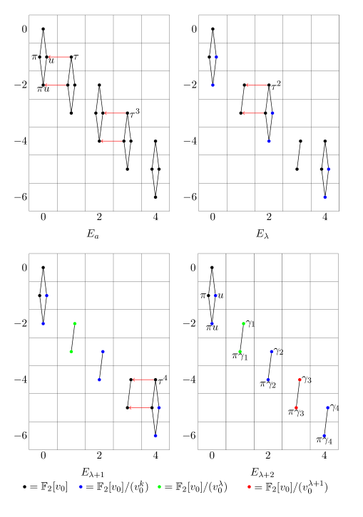
Figure 2. The mASS for $\mathsf{BPGL}\langle 0\rangle$ over $F$

We now use this information about the mASS for $\mathsf{BPGL}\langle 0\rangle$ to compute $\pi_{\star}\mathsf{BPGL}\langle n\rangle\,\widehat{{}_{2}}$. The surprising fact is that, for $i>0$, the differentials have no $v_{i}$-components so that $E_{r}(\mathsf{BPGL}\langle n\rangle)=E_{r}(\mathsf{BPGL}\langle 0\rangle)[v_{1},\ldots,v_{n}]$.

Theorem 5.5.

The differentials in the mASS for $\mathsf{BPGL}\langle n\rangle$ are identical to those for $\mathsf{BPGL}\langle 0\rangle$ in Theorem 5.2.

Proof.

Note that all the $v_{i}$ and elements in $k^{M}_{*}(F)$ are permanent cycles. (This is obvious since their target ranges are trivial; see Figure 3.) Inductively, then, we can show that

$$E_{r}(\mathsf{BPGL}\langle n\rangle)=E_{r}(\mathsf{BPGL}\langle 0\rangle)[v_{1},\ldots,v_{n}].$$

The result is true on $E_{2}$ pages; assume it is true on $E_{r}$ and consider the map $f$ of spectral sequences induced by $\mathsf{BPGL}\langle n\rangle\to\mathsf{BPGL}\langle 0\rangle$. By dimensional accounting, it is clear that the $E_{r+1}$-page is determined by the differential on the smallest surviving $\tau$-power. The map $f$ is an isomorphism on the target of this $\tau$-power by dimensional accounting. Indeed, since $cd_{2}(F)=2$ (i.e. $k^{M}_{*}(F)$ is only nonzero for $0\leq*\leq 2$) no $v_{>0}$-terms can appear in the target. This proves that the $\tau$-power supports the same differential as in the mASS for $\mathsf{BPGL}\langle 0\rangle$, from which we get the result on $E_{r+1}$. ∎

Remark 5.6.

The mASS for $\mathsf{BPGL}\langle n\rangle$ is depicted in Figure 3. The grading convention described in Remark 5.4 is followed again. Note that the arrows with slope 1 represent multiplication by $v_{i}$’s, $i>0$, and they also come “out of the page” since $v_{i}$ has homological degree 1. Note the obvious vanishing region with $k^{M}_{*}(F)$ and the $v_{i}$ monomials on the boundary.

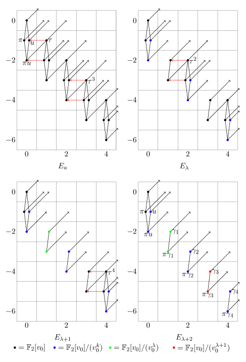
Figure 3. The mASS for $\mathsf{BPGL}\langle n\rangle$ over $F$

We now have the following unified description of the $E_{\infty}$ page of the mASS for $\mathsf{BPGL}\langle n\rangle$, $0\leq n\leq\infty$.

Theorem 5.7.

Let $a=\nu_{2}(q-1)$ and let $\lambda=\nu_{2}(q^{2}-1)$. The $E_{\infty}$-term of the mASS for $\mathsf{BPGL}\langle n\rangle$ over a $p$-adic field $F$ is

$$\Gamma^{\prime}[v_{1},\ldots,v_{n}]$$

where $\Gamma^{\prime}$ has additive structure

$$\Gamma^{\prime}=\begin{cases}\mathbb{Z}/2[v_{0}]&\text{in dimension }0,\\ \mathbb{Z}/2[v_{0}]\left\{\pi\right\}\oplus\mathbb{Z}/2[v_{0}]/v_{0}^{a}\left\{u\right\}&\text{in dimension }-\alpha,\\ \mathbb{Z}/2[v_{0}]/v_{0}^{a}\left\{\pi u\right\}&\text{in dimension }-2\alpha,\\ \mathbb{Z}/2[v_{0}]/v_{0}^{\lambda-1+\nu_{2}(i)}\left\{\gamma_{i}\right\}&\text{in dimension }i(1-\alpha)-\alpha\\ &\text{for }i\text{ odd},\\ \mathbb{Z}/2[v_{0}]/v_{0}^{\lambda-1+\nu_{2}(i)}\left\{\pi\gamma_{i}\right\}&\text{in dimension }i(1-\alpha)-2\alpha\\ &\text{for }i\text{ odd},\\ \mathbb{Z}/2[v_{0}]/v_{0}^{a}\left\{\gamma_{i}\right\}&\text{in dimension }i(1-\alpha)-\alpha\\ &\text{for }i\text{ even},\\ \mathbb{Z}/2[v_{0}]/v_{0}^{a}\left\{\pi\gamma_{i}\right\}&\text{in dimension }i(1-\alpha)-2\alpha\\ &\text{for }i\text{ odd},\\ 0&\text{otherwise}.\end{cases}$$

The generators in each degree are indicated above. They satisfy the obvious multiplicative relations indicated by their notation while $u\gamma_{i}$ and $\gamma_{i}\gamma_{j}$ are 0. ∎

A quick inspection of tri-degrees reveals that there are no extensions except those created by $v_{0}$-multiplication. Indeed, the lines of slope 1 originating in the nontrivial dimensions of $\Gamma^{\prime}$ do not overlap, so we only need to worry about $v_{0}$-towers. Since $v_{0}$ represents 2 in $\pi_{0}\mathsf{BPGL}\langle n\rangle\,\widehat{{}_{2}}$, any copies of $\mathbb{Z}/2[v_{0}]$ produce copies of the 2-adic integers $\mathbb{Z}_{2}$, and any copies of $\mathbb{Z}/2[v_{0}]/v_{0}^{b}$ produce copies of $\mathbb{Z}/2^{b}$. This proves the following theorem.

Theorem 5.8.

Let $a=\nu_{2}(q-1)$, $\lambda=\nu_{2}(q^{2}-1)$ and set $w_{i}=\mathbb{Z}/2^{a}$ for $i$ odd, $w_{i}=2^{\lambda-1+\nu(i)}$ for $i$ even. The coefficients of the 2-complete algebraic Johnson-Wilson spectra $\mathsf{BPGL}\langle n\rangle\,\widehat{{}_{2}}$ over a $p$-adic field $F$ are

$$\pi_{\star}\mathsf{BPGL}\langle n\rangle\,\widehat{{}_{2}}=(\pi_{\star}\mathsf{BPGL}\langle 0\rangle\,\widehat{{}_{2}})[v_{1},v_{2},\ldots]$$

where $|v_{i}|=(2^{i}-1)(1+\alpha)$ and, additively,

$$\pi_{\star}\mathsf{BPGL}\langle 0\rangle\,\widehat{{}_{2}}=\begin{cases}\mathbb{Z}_{2}&\text{in dimension }0,\\ \mathbb{Z}_{2}\oplus\mathbb{Z}/w_{1}&\text{in dimension }-\alpha,\\ \mathbb{Z}/w_{1}&\text{in dimension }-2\alpha,\\ \mathbb{Z}/w_{i}&\text{in dimension }(i-1)(1-\alpha)-\epsilon\alpha\\ &\text{ for }i\geq 1\text{ and }\epsilon=1\text{ or }2,\\ 0&\text{otherwise}.\end{cases}$$

Multiplicative structure and generator names for $\pi_{\star}\mathsf{BPGL}\langle 0\rangle\,\widehat{{}_{2}}$ are the same as in Theorem 5.7. ∎

Corollary 5.9.

The coefficients of the 2-complete algebraic cobordism spectrum over a $p$-adic field $F$ are

$$\pi_{\star}\mathsf{MGL}\,\widehat{{}_{2}}=\Gamma[x_{1},x_{2},\ldots]$$

where $|x_{i}|=i(1+\alpha)$. ∎

Corollary 5.10.

Over a $p$-adic field, the slice spectral sequences for $\mathsf{MGL}\,\widehat{{}_{2}}$ and $\mathsf{BPGL}\langle n\rangle\,\widehat{{}_{2}}$ ($0\leq n\leq\infty$) collapse.

Proof.

Hopkins-Morel show that the slice associated gradeds for $\mathsf{MGL}$ and $\mathsf{BPGL}\langle n\rangle$ are $H\mathbb{Z}_{\star}[x_{1},x_{2},\ldots]$, $H\mathbb{Z}_{\star}[v_{1},\ldots,v_{n}]$, respectively, and Theorem 5.8 implies that there are no differentials in the slice spectral sequences for their 2-completions. ∎

Corollary 5.11.

The coefficients of 2-complete $\mathsf{kgl}$ are $(\pi_{\star}\mathsf{BPGL}\langle 0\rangle)[v_{1}]$. In particular, there is no $v_{1}$-torsion and we recover the 2-complete algebraic $K$-theory of $F$ in degrees $m+0\alpha$.

We conclude by discussing some easy corollaries of this work that highlight the importance of the algebraic Brown-Peterson spectra and have important applications to the motivic ANSS [Orm10, Orm]. See [HKO10, HKO, DI10] for discussions of the motivic Adams-Novikov spectral sequence.

For convenience, let $\Gamma\mathrel{\mathop{:}}=\pi_{\star}\mathsf{BPGL}\langle 0\rangle\,\widehat{{}_{2}}=\pi_{\star}H\mathbb{Z}_{2}$. For typographical simplicity, we drop the 2-completion $(~{})\,\widehat{{}_{2}}$ from our notation in the rest of this section.

Theorem 5.12.

Fix a $p$-adic field $F$ and work in the 2-complete stable motivic homotopy category over $F$. Then the Hopf algebroid for $\mathsf{BPGL}$ splits as

$$(\mathsf{BPGL}_{\star},\mathsf{BPGL}_{\star}\mathsf{BPGL})=(\mathsf{BP}_{*},\mathsf{BP}_{*}\mathsf{BP})\otimes_{\mathbb{Z}_{2}}\Gamma.$$

Moreover, the $E_{2}$-term of the motivic ANSS in homological degree $s$ is

$$\operatorname{Ext}^{s}_{\mathsf{BPGL}_{\star}\mathsf{BPGL}}(\mathsf{BPGL}_{\star},\mathsf{BPGL}_{\star})=\begin{array}[]{c}{}^{\operatorname{top}}E_{2}^{s}\otimes_{\mathbb{Z}_{2}}\Gamma\\ \oplus\\ \operatorname{Tor}^{\mathbb{Z}_{2}}_{1}({}^{\operatorname{top}}E_{2}^{s+1},\Gamma)\end{array}.$$

Here ${}^{{\operatorname{top}}}E_{2}=\operatorname{Ext}_{\mathsf{BP}_{*}\mathsf{BP}}(\mathsf{BP}_{*},\mathsf{BP}_{*})$ with degrees shifted so that elements appearing in degree $(s,2m)$ in topology appear in degree $(s,m(1+\alpha))$ motivically.

Proof.

The second statement is an easy consequence of the first via the cobar resolution computing $\operatorname{Ext}_{\mathsf{BPGL}_{\star}\mathsf{BPGL}}(\mathsf{BPGL}_{\star},\mathsf{BPGL}_{\star})$ and the universal coefficient theorem.

As a consequence of motivic Landweber exactness, Naumann-Østvær-Spitzweck [NSØ09] deduce a splitting of the $\mathsf{MGL}$ Hopf algebroid as

$$(\mathsf{MGL}_{\star},\mathsf{MGL}_{\star}\mathsf{MGL})=(\mathsf{MU}_{*},\mathsf{MU}_{*}\mathsf{MU})\otimes_{\mathsf{MU}_{*}}\mathsf{MGL}_{\star}$$

where $\mathsf{MU}_{*}$ is the coefficients of (topological) complex cobordism, the Lazard ring. This splitting passes to $\mathsf{BPGL}$, so

$$(\mathsf{BPGL}_{*},\mathsf{BPGL}_{*}\mathsf{BPGL}) =(\mathsf{BP}_{*},\mathsf{BP}_{*}\mathsf{BP})\otimes_{\mathsf{BP}_{*}}\mathsf{BPGL}_{\star}$$

$$=(\mathsf{BP}_{*},\mathsf{BP}_{*}\mathsf{BP})\otimes_{\mathsf{BP}_{*}}(\mathsf{BP}_{*}\otimes_{\mathbb{Z}_{2}}\Gamma)$$

$$=(\mathsf{BP}_{*},\mathsf{BP}_{*}\mathsf{BP})\otimes_{\mathbb{Z}_{2}}\Gamma.$$

∎

This description of the $E_{2}$-term of the motivic ANSS over $F$ already pays dividends in the form of a graded algebra with infinitely many nonzero components previously undiscovered in the stable stems $\pi_{\star}\mathbbm{1}\,\widehat{{}_{2}}$ of the 2-complete sphere spectrum.

Theorem 5.13.

The algebra $\Gamma$ survives to $E_{\infty}$ of the motivic Adams-Novikov spectral sequence and represents a copy of $(H\mathbb{Z}_{2})_{\star}$ in $\pi_{\star}\mathbbm{1}\,\widehat{{}_{2}}$.

Proof.

The elements of $\Gamma=E_{2}^{0,0}\otimes\Gamma$ are in filtration 0 and hence are not the targets of differentials. We must show that elements of $\Gamma$ do not support differentials. For an element of degree $(s,m+n\alpha)$ in $E_{2}$, call $m+n-s$ the classical Adams degree. Since $\Gamma$ is concentrated in classical Adams degrees $0,-1$, and $-2$, Theorem 5.12 gives a vanishing line $E_{2}^{s,m+n\alpha}=0$ for $s>m+n-s+2$. Differentials in the motivic ANSS decrease classical Adams degree by 1 and increase homological degree by at least 2. Since $\Gamma$ has $s=0$ and classical Adams degree $0,-1$, and $-2$, we see that it does not support differentials. ∎

References

• [Bor03] Simone Borghesi, Algebraic Morava $K$-theories, Invent. Math. 151 (2003), no.Β 2, 381–413.
• [Cas86] J.Β W.Β S. Cassels, Local fields, London Mathematical Society Student Texts, vol.Β 3, Cambridge University Press, Cambridge, 1986.
• [DI10] Daniel Dugger and DanielΒ C. Isaksen, The motivic Adams spectral sequence, Geom. Topol. 14 (2010), no.Β 2, 967–1014.
• [DRØ03] BjΓΈrnΒ Ian Dundas, Oliver RΓΆndigs, and PaulΒ Arne ØstvΓ¦r, Motivic functors, Doc. Math. 8 (2003), 489–525 (electronic).
• [Hill] MichaelΒ A. Hill, Ext and the motivic steenrod algebra over ${\mathbb{R}}$, arXiv:0904.1998.
• [HK01] PoΒ Hu and Igor Kriz, Some remarks on Real and algebraic cobordism, $K$-Theory 22 (2001), no.Β 4, 335–366.
• [HKO] PoΒ Hu, Igor Kriz, and KyleΒ M. Ormsby, Convergence of the motivic Adams spectral sequence, J. of $K$-theory 7 (2011).
• [HKO10] by same author, Remarks on motivic homotopy theory over algebraically closed fields, J. of $K$-theory (2010), doi:10.1017/is010001012jkt098.
• [Hu03] PoΒ Hu, $S$-modules in the category of schemes, Mem. Amer. Math. Soc. 161 (2003), no.Β 767, viii+125.
• [IS] DanielΒ C. Isaksen and Armira Shkembi, Motivic connective $K$-theories and the cohomology of $A(1)$, arXiv:1002.2638.
• [Jar00] J.Β F. Jardine, Motivic symmetric spectra, Doc. Math. 5 (2000), 445–553 (electronic).
• [May70] J.Β Peter May, A general algebraic approach to Steenrod operations, The Steenrod Algebra and its Applications (Proc. Conf. to Celebrate N. E. Steenrod’s Sixtieth Birthday, Battelle Memorial Inst., Columbus, Ohio, 1970), Lecture Notes in Mathematics, Vol. 168, Springer, Berlin, 1970, pp.Β 153–231.
• [Mil70] John Milnor, Algebraic $K$-theory and quadratic forms, Invent. Math. 9 (1969/1970), 318–344.
• [Mil71] by same author, Introduction to algebraic $K$-theory, Princeton University Press, Princeton, N.J., 1971, Annals of Mathematics Studies, 72.
• [Mor04] Fabien Morel, On the motivic $\pi_{0}$ of the sphere spectrum, Axiomatic, enriched and motivic homotopy theory, NATO Sci. Ser. II Math. Phys. Chem., 131, Kluwer Acad. Publ., Dordrecht, 2004, pp.Β 219–260.
• [Mor05] by same author, The stable ${\mathbb{A}}^{1}$-connectivity theorems, $K$-Theory 35 (2005), no.Β 1-2, 1–68.
• [MV99] Fabien Morel and Vladimir Voevodsky, ${\bf A}^{1}$-homotopy theory of schemes, Inst. Hautes Γ‰tudes Sci. Publ. Math. 90 (1999), 45–143 (2001).
• [NSØ09] Niko Naumann, Markus Spitzweck, and PaulΒ Arne ØstvΓ¦r, Motivic Landweber exactness, Doc. Math. 14 (2009), 551–593.
• [Orm] KyleΒ M. Ormsby, The ${K}(1)$-local motivic sphere, in preparation.
• [Orm10] by same author, Computations in stable motivic homotopy theory, Ph.D. thesis, University of Michigan, 2010.
• [Rav86] DouglasΒ C. Ravenel, Complex cobordism and stable homotopy groups of spheres, Pure and Applied Mathematics, 121, Academic Press Inc., Orlando, FL, 1986.
• [RW00] J.Β Rognes and C.Β Weibel, Two-primary algebraic $K$-theory of rings of integers in number fields, J. Amer. Math. Soc. 13 (2000), no.Β 1, 1–54, Appendix A by Manfred Kolster.
• [SØ09] Markus Spitzweck and PaulΒ Arne ØstvΓ¦r, The Bott inverted infinite projective space is homotopy algebraic $K$-theory, Bull. Lond. Math. Soc. 41 (2009), no.Β 2, 281–292.
• [Vez01] Gabriele Vezzosi, Brown-Peterson spectra in stable $\mathbb{A}^{1}$-homotopy theory, Rend. Sem. Mat. Univ. Padova 106 (2001), 47–64.
• [Voe] Vladimir Voevodsky, Motivic Eilenberg-MacLane spaces, arXiv:0805.4432.
• [Voe98] by same author, $\mathbb{A}^{1}$-homotopy theory, Proceedings of the International Congress of Mathematicians, Vol. I (Berlin, 1998), no. Extra Vol. I, 1998, pp.Β 579–604 (electronic).
• [Voe03a] by same author, Motivic cohomology with ${\bf Z}/2$-coefficients, Publ. Math. Inst. Hautes Γ‰tudes Sci. 98 (2003), 59–104.
• [Voe03b] by same author, Reduced power operations in motivic cohomology, Publ. Math. Inst. Hautes Γ‰tudes Sci. 98 (2003), 1–57.
• [Wil75] W.Β Stephen Wilson, The $\Omega$-spectrum for Brown-Peterson cohomology. II, Amer. J. Math. 97 (1975), 101–123.