Investigation on Vibrational, Optical and Structural Properties of an Amorphous Se_0.80S_0.20 Alloy Produced by Mechanical Alloying

Abstract

An amorphous Se_0.80S_0.20 alloy produced by Mechanical Alloying was studied by Raman spectroscopy, x-ray diffraction, extended x-ray absorption fine structure (EXAFS) and optical absorption spectroscopy, and also through reverse Monte Carlo simulations of its total structure factor and EXAFS data. Its vibrational modes, optical gap and structural properties as average interatomic distances and average coordination numbers were determined and compared to those found for an amorphous Se_0.90S_0.10 alloy. The results indicate that coordination numbers, interatomic distances and also the gap energy depend on the sulphur concentration.

1 Introduction

Owning to their technological applications in optoelectronic, optical, electronic and memory switching devices the research on chalcogenide glasses formed by elements Se, S and Te has increased in recent years. Usually, chalcogenide alloys based on selenium have high transparency in the broad middle and far infrared region and have strong non-linear properties. Alloys formed by Se and S exhibits an electronic conductivity of p-type semiconductor and some properties related to these alloys were already studied. Thermal and electrical properties for amorphous samples were determined in some studies Kotkata1 ; Kotkata2 ; Mahmoud , and recently Musahwar et al. Musahwar measured dielectric and electrical properties for Se_xS_1-x glasses ($x=1,0.95,0.90,0.85,0.80$), and the optical gap of Se_xS_1-x thin films ($x=0.9,0.8,0.7,0.6$) were determined by Rafea and Farag Rafea . Ward Ward obtained vibrational modes for some crystalline Se-S alloys through Raman spectroscopy. Concerning structural properties, relatively few investigations have been done on these alloys. The compositional range for fabrication of amorphous Se-S alloys was studied by Kotkata et al. Kotkata3 ; Kotkata4 through x-ray diffraction (XRD) measurements. They produced several amorphous and crystalline Se_xS_1-x alloys and obtained some general results, indicating that amorphous alloys can be prepared in a relatively wide compositional range, from $x=0.5$ to $x=1$, the density of the alloys decreases as the S content is increased and the average total coordination number for Se atoms ($\langle N^{\text{Se}}\rangle=\langle N^{\text{Se-Se}}\rangle+\langle N^{\text{Se-S}}\rangle$) is 2. Heiba et al. Heiba also used the XRD technique to study the crystallization of Se_xS alloys, $x=20,30,40$, and crystallite sizes were determined from a refinement using the program FULLPROOF. A more detailed investigation of amorphous alloys was made by Shama Shama , which reports the results obtained from simulations of the first shell of the radial distribution functions (RDF) determined for three amorphous Se_xS alloys, $x=10,30,40$. For these alloys, average coordination numbers and average interatomic distances for Se-Se pairs were determined, but the existence of Se-S pairs was not considered. The values found were $\langle N^{\text{Se-Se}}\rangle=2.10$ and $\langle r^{\text{Se-Se}}\rangle=2.369$ Å, for Se₁₀S, and $\langle N^{\text{Se-Se}}\rangle=2.14$ and $\langle r^{\text{Se-Se}}\rangle=2.368$ Å for Se₃₀S. It is interesting to note that all samples cited were prepared by quenching, except those in Rafea , which were prepared by thermal evaporation. Fukunaga et al. Fukunaga2 used the Mechanical Alloying (MA) MASuryanarayana technique to produce amorphous Se_xS_1-x alloys, in the compositions $x=1,0.90,0.80,0.70,0.60$, which were investigated using neutron diffraction (ND) followed by a RDF analysis. However, results were given only for the composition Se_0.60S_0.40, and, in this case, they found $\langle N^{\text{Se-Se}}\rangle=1.78\pm 0.018$ and $\langle r^{\text{Se-Se}}\rangle=2.37\pm 0.002$ Å, and again the possibility of having Se-S pairs was not taken into account. In addition, they assumed that the MA process only mixed Se chains and S rings, and there is no alloying at the atomic level.

Due to the promising applications of Se-S alloys and the lack of a sistematic investigation of their structures, we started a more detailed structural study about this alloys. In a recent article klese90s10 we investigated an amorphous Se_0.90S_0.10 alloy (a-Se_0.90S_0.10) produced by MA. We obtained vibrational properties, by Raman spectroscopy, optical properties, by optical absorption spectroscopy, and structural properties considering extended x-ray absorption fine structure spectroscopy (EXAFS) and synchrotron XRD. We also made reverse Monte Carlo (RMC) simulations rmcreview ; rmc++ of the total structure factor ${\mathcal{S}}(K)$ obtained from the XRD data.

In the present study, we analized the formation of an amorphous Se_0.80S_0.20 alloy (a-Se_0.80S_0.20) also produced by MA, and investigated its vibrational modes using Raman spectroscopy, its structural properties considering RMC simulations using both XRD ${\mathcal{S}}(K)$ and EXAFS $\chi(k)$ signal at Se K edge as input data and we also determined the optical gap by optical absorption spectroscopy. All data were compared to those obtained for a-Se_0.90S_0.10 and some interesting features can be inferred from the data obtained.

2 Experimental Procedures

Amorphous Se_0.80S_0.20 samples were produced by milling Se (Aldrich, purity $>$ 99.99%) and S (Vetec, purity $>$ 99.5%) powders in the composition above. The powders were sealed together with 15 steel balls (diameter 10 mm), under argon atmosphere, in a steel vial. The weight ratio of the ball to powder was 9:1. The vial was mounted in a Fritsch Pulverisette 5 planetary ball mill and milled at 350 rpm. In order to keep the vial temperature close to room temperature, the milling was performed considering cycles of 20 min of effective milling followed by 10 min of rest. To investigate the formation of the alloy, XRD measurements were taken after 11 h, 23 h, 34 h, 46 h and 57 h of milling. They were done in a Shimadzu difractometer using Cu K_α radiation ($\lambda=1.5418$ Å) in a $\theta$–$2\theta$ scanning mode, considering a $\Delta 2\theta$ step of 0.04^∘ and each $2\theta$ point was measured during 22 s for all milling times except for 11 h, which was measured considering 1 s per point. After 57 h of milling, the XRD pattern was characteristic of amorphous samples, showing large amorphous halos without crystalline peaks.

Micro-Raman measurements were performed with a Renishaw spectrometer coupled to an optical microscope and a cooled CCD detector. The 6238 Å line of an HeNe laser was used as exciting light, always in backscattering geometry. The output power of the laser was kept at about 1–3 mW to avoid overheating samples. All Raman measurements were performed with the samples at room temperature.

EXAFS measurements at Se K edge were taken at room temperatures in the transmission mode at beam line D08B - XAFS2 of the Brazilian Synchrotron Light Laboratory - LNLS (Campinas, Brazil). Three ionization chambers were used as detectors. The a-Se_0.80S_0.20 sample was formed by placing the powder onto a porous membrane (Millipore, 0.2 $\mu$m pore size) in order to achieve optimal thickness (about 50 $\mu$m) and it was placed between the first and second chambers. A crystalline Se foil used as energy reference was placed between the second and third chambers. The beam size at the sample was 3 $\times$ 1 mm. The energy and average current of the storage ring were 1.37 GeV and 190 mA, respectively.

In order to obtain the EXAFS $\chi(k)$ signal on Se K edge to be used on RMC simulations, the raw EXAFS data were analyzed following standard procedures. EXAFS spectra were energy calibrated, aligned, and isolated from raw absorbance performing a background removal using the AUTOBK algorithm of the ATHENA athena program, and the $\chi(k)$ signal was obtained.

Synchrotron XRD measurements were carried out at the BW5 beamline Palref at HASYLAB. All data were taken at room temperature using a Si (111) monochromator and a Ge solid state detector. The energy of the incident beam was 121.3 keV ($\lambda=0.102$ Å), and it was calibrated using a LaB₆ standard sample. The uncertainty in the wavelength is less than 0.5%. The cross section of the beam was $1\times 4$ mm² (h x v). Powder sample was filled into a thin walled (10 $\mu$m) quartz capillary with 2 mm diameter. The energy and average current of the storage ring were 4.4 GeV and 110 mA, respectively. Raw intensity was corrected for deadtime, background, polarization, detector solid angle and Compton-scattering as described in Palref . The total structure factor was computed from the normalized intensity $I_{a}(K)$ according to Faber and Ziman Faber (see eq. 1).

Absorbance measurements were carried out in a Shimadzu UV-2401-PC spectrometer. In these measurements the a-Se_0.80S_0.20 sample was mixed to KBr and pressed in the form of a pellet. KBr was used as support and reference.

3 Theoretical Background

3.1 Structure Factors and RMC Simulations

According to Faber and Ziman Faber , the total structure factor ${\mathcal{S}}(K)$ is obtained from the scattered intensity per atom $I_{a}(K)$ through

$${\mathcal{S}}(K) = \frac{I_{a}(K)-\bigl{[}\langle f^{2}(K)\rangle-\langle f(K)\rangle^{2}\bigr{]}}{\langle f(K)\rangle^{2}}\,,$$ (1)

$${\mathcal{S}}(K) = \sum_{i=1}^{n}{\sum_{j=1}^{n}{w_{ij}(K){\mathcal{S}}_{ij}(K)}}\,,$$ (2)

where $K$ is the transferred momentum, ${\mathcal{S}}_{ij}(K)$ are the partial structure factors and $w_{ij}(K)$ are given by

$$w_{ij}(K)=\frac{c_{i}c_{j}f_{i}(K)f_{j}(K)}{\langle f(K)\rangle^{2}}\,,$$ (3)

and

$$\langle f^{2}(K)\rangle = \sum_{i}{c_{i}f_{i}^{2}(K)}\,,$$

$$\langle f(K)\rangle^{2} = \Bigl{[}\sum_{i}{c_{i}f_{i}(K)}\Bigr{]}^{2}\,.$$

Here, $f_{i}(K)$ is the atomic scattering factor and $c_{i}$ is the concentration of atoms of type $i$. The partial distribution functions $g_{ij}(r)$ are related to ${\mathcal{S}}_{ij}(K)$ and ${\mathcal{S}}(K)$ through

$$g_{ij}(r)=\frac{2}{\pi}\int_{0}^{\infty}{K\bigl{[}{\mathcal{S}}_{ij}(K)-1\bigr{]}\sin(Kr)\,dK}\,,$$ (4)

and, from these functions, interatomic distances and coordination numbers can be determined.

The structure factors defined by eq. 1 can be used in RMC simulations. The algorithm of the standard RMC method are described elsewhere rmcreview ; rmc++ and its application to different materials is reported in the literature nitikleber ; Pal1 ; rmcNDXRD ; Iparraguirre .

When using XRD data only, the idea is to minimize the function

$$\psi^{2}_{\text{XRD}}=\sum_{i=1}^{m}{\frac{\bigl{[}{\mathcal{S}}^{\rm{RMC}}(K_{i})-{\mathcal{S}}(K_{i})\bigr{]}^{2}}{\delta^{2}_{\text{XRD}}}}$$ (5)

where ${\mathcal{S}}(K)$ is the experimental total structure factor, ${\mathcal{S}}^{\rm{RMC}}(K)$ is the estimate of ${\mathcal{S}}(K)$ obtained by RMC simulations, $\delta_{\text{XRD}}$ is a parameter related to the convergence of the simulations and to the experimental errors and the sum is over $m$ experimental points. In our case, we added EXAFS data to the simulations, and the function

$$\psi^{2}=\psi^{2}_{\text{XRD}}+\psi^{2}_{\text{EXAFS}}$$ (6)

where

$$\psi^{2}_{\text{EXAFS}}=\sum_{i=1}^{m}{\frac{\bigl{[}\chi^{\rm{RMC}}(k_{i})-\chi(k_{i})\bigr{]}^{2}}{\delta^{2}_{\text{EXAFS}}}}$$ (7)

is the function to be minimized. In eq. 7, $\chi(k_{i})$ is the experimental EXAFS signal, $\chi^{\rm{RMC}}(k)$ is its estimate obtained using RMC simulations and $\delta_{\text{EXAFS}}$ is the parameter related to the experimental errors in the EXAFS signal. To perform the simulations we have considered the RMC program available on the Internet rmc++ and cubic cells with 16000 atoms. The total structure factor obtained from XRD measurements and the EXAFS data at Se K edge were used as input data for the simulations.

3.2 Optical Band Gap Determination

To obtain the optical gap a simple and direct procedure can be used, and consists in determining the wavelength at which the extrapolations of the baseline and the absorption edge cross Boldish . A more sofisticated approach makes use of a McLean analysis McLean of the absorption edge, which furnishes more information about the lowest energy interband transition. The absorption coefficient $\alpha$ follows the equation

$$\alpha h\nu=(h\nu-E_{g})^{\frac{1}{n}}$$ (8)

where $E_{g}$ is the gap energy and $\nu$ is the frequency of the incident beam. The analysis consists of fitting the absorption edge to eq. 8 and determining experimental values for $E_{g}$ and $n$. $n=2$ correponds to a direct allowed transition. $n=\frac{2}{3}$ implies a direct forbidden transition. $n=\frac{1}{2}$ is associated with an indirect allowed transition and $n=\frac{1}{3}$ implies an indirect forbidden transition. The absorbance $A$, the absorption coefficient $\alpha$ and the thickness $d$ of a sample are related by $\alpha=A/d$ and, for absorbance measurements on powders, in which the polycrystalline or amorphous samples are dispersed into a powder support such as KBr, the mixture is pressed in the form of pellet. In this case, the thickness $d$ and the absorption coefficient $\alpha$ of the sample become unknown. Thus, eq. 8 must be modified to

$$Ah\nu=C(h\nu-E_{g})^{\frac{1}{n}}$$ (9)

where $C$ represents the thickness of the sample and is a parameter to be included in the fitting procedure.

4 Results and Discussion

4.1 Formation of a-Se_0.80S_0.20

In order to compare the evolution with milling time of a-Se_0.80S_0.20 and a-Se_0.90S_0.10 we stopped the milling at some chosen times and made conventional XRD measurements to verify the changes on the structure of the alloy. Fig. 1 shows these XRD measurements obtained for a-Se_0.80S_0.20. In this figure the XRD pattern for the crystalline selenium powder (c-Se) used as the starting material is also shown for comparison.

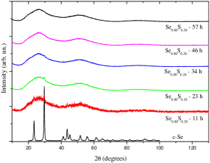
Figure 1: XRD measurements obtained for a-Se_0.90S_0.10 after selected milling times: 11 h, 23 h, 34 h, 46 h and 57 h. The XRD pattern for c-Se is also shown for comparison.

We decided to make the first stop after 11 h of milling. Considering the results obtained for a-Se_0.90S_0.10 (fig. 1 of Ref. klese90s10 ), we supposed that at this time an intermediate structural state between those found at 4 h and at 14 h of milling would be found and, in fact, the XRD pattern for a-Se_0.80S_0.20 at 11 h of milling corroborates this assumption.

The next stop was at 23 h, and the XRD pattern shows only the most intense crystalline Se peak around 30^∘, besides the amorphous halos, being similar to the XRD pattern at 25 h of milling for a-Se_0.90S_0.10. Then we decided to make more stops, to verify the evolution of the remaining Se peak. At 34 h this peak was still seen in the XRD pattern, and disappeared only after 46 h of milling. After that, the amorphous structure is stable, as the XRD pattern at 57 h indicates.

It is interesting to note that, according Fukunaga et al. Fukunaga2 , after 30 h of milling the a-Se_0.80S_0.20 alloy should be ready. Since MA is very sensitive to the milling conditions MASuryanarayana , and considering that we used a different number of balls and a different total mass of the starting powders, resulting in a free volume inside the vial larger to us than to them, we believe these points explain the difference in the milling time needed to produce the alloy.

4.2 Raman Spectroscopy Results

In their study about Se-S amorphous alloys, Fukunaga et al. Fukunaga2 stated that MA produces only a mixing of Se chains and S rings and not a true alloy at the atomic level. This idea was also assumed by Shama Shama , for a quenched sample. However, we have demonstrated that this assumption is wrong for a-Se_0.90S_0.10 klese90s10 , since some Raman modes related to Se-S vibrations appear in the Raman spectrum of this alloy. Thus, we expected that for a-Se_0.80S_0.20 these vibrations would also appear, besides some shifts on the other modes associated with Se-Se vibrations. Fig. 2 shows the results obtained for this alloy, for amorphous Se, for c-S and also for a-Se_0.90S_0.10, for comparison.

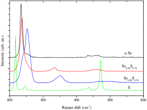
Figure 2: Raman spectra for a-Se_0.80S_0.20, a-Se_0.90S_0.10, a-Se and c-S.

Fig. 2 shows clearly that some vibrational modes associated with a-Se appear in a-Se_0.90S_0.10 and a-Se_0.80S_0.20, but some features change as the concentration of sulphur increases. The peak around 234 cm^-1 (which is usually associated with Se chains Luo ) decreases and that at 250 cm^-1 (associated to Se rings Luo ) increases indicating structural modifications on Se-Se units as sulphur is introduced on crystalline Se chains. In addition, the large band seen around 460 cm^-1 in a-Se_0.90S_0.10 is located in a-Se_0.80S_0.20 at 490 cm^-1.

These modes also appear in other Se-based alloys KleGeSe ; GaSeRaman ; Sugai . The more interesting modes, however, are those associated with the broad peak around 334 cm^-1 in a-Se_0.90S_0.10 and around 352 cm^-1 in a-Se_0.80S_0.20, which cannot be associated with Se-Se vibrations, either in crystalline or amorphous Se, or with S-S vibrations. Ward Ward obtained RS measurements for Se_0.05S_0.95 and Se_0.33S_0.67 crystalline alloys and found three Se-S modes in this region, at 344 cm^-1, 360 cm^-1 and 380 cm^-1. Thus, the conclusion is that Se-S pairs are found in our alloy, besides Se-Se and S-S ones and, since the relative intensity of the modes in this region is increasing, we could expect an increase in the contribution of Se-S vibrations, and probably an increase in the Se-S average coordination number. By fitting the Raman peaks using Lorentzian functions we have determined the Raman modes given in table 1.

Table 1: Raman modes obtained from fitting the peaks seen at fig. 2 to Lorentzian functions and their occurence in c-Se, a-Se and Se-S alloys.

Mode	Frequency	Mode
	(cm-1)	found in
$A_{1}$, $E$	239	c-Se and a-Se
$A_{2}$, $E$	253	c-Se and a-Se
$A_{1}$	338	c-Se0.33S0.67
$A_{1}$	352	c-Se0.33S0.67 and c-Se0.05S0.95
$A_{1}$	445	c-Se0.33S0.67 and c-Se0.05S0.95
		and also c-Se and a-Se
$A_{1}$	465	c-Se0.33S0.67 and c-Se0.05S0.95
		c-Se and a-Se
$A_{1}$	498	c-Se0.33S0.67 and c-Se0.05S0.95
		c-Se and a-Se

4.3 RMC Simulations

To obtain structural data as average coordination numbers and average interatomic distances, we made RMC simulations rmcreview ; rmc++ using the total structure factor ${\mathcal{S}}(K)$ obtained from XRD measurements through eq. 1 and also the EXAFS $\chi(k)$ signal at Se K edge. The first point is to determine the density of the alloy. To do that, we used the procedure suggested in Ref. Gereben , and made several simulations for different values of the density $\rho$ keeping minimum distances and $\delta$ fixed (see eqs. 5 and 7). Thus, we chose the density that minimized the $\psi^{2}_{eq}$ parameter, which was $\rho=0.030$ atm/ų. It should be noted that the density found for a-Se_0.90S_0.10 had the same value at least considering the error bars. Then, we made several simulations changing the minimum distances between atoms, in order to find the best values for these parameters. All the simulations performed followed the procedure below

1. First, hard sphere simulation without experimental data were made to avoid possible memory effects of the initial configurations in the results. These simulations were run until reaching at least $3\times 10^{6}$ accepted moves.

2. Next, simulations using the XRD experimental data were performed to obtain an initial convergence.

3. Finally, the EXAFS signal was added to the simulations. After reaching the convergence the statistically independent configurations were collected considering at least $1\times 10^{5}$ accepted movements between one configuration and the next. At the end of the simulations, about 33% of the generated movements were accepted.

The best values obtained for the minimum distances were $r_{min}=2.20$ Å for Se-Se and Se-S pairs and $r_{min}=2.00$ Å for S-S pairs. The experimental total structure factor ${\mathcal{S}}(K)$ and its RMC simulation obtained considering these values, 16000 atoms and the density found are shown in fig. 3. As it can be seen, a very good agreement between them is reached.

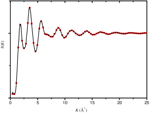
Figure 3: Experimental (full black line) and simulated (red squares) total structure factor for a-Se_0.80S_0.20.

Fig. 4 shows the EXAFS $k^{3}\chi(k)$ signal and its RMC simulation. Again there is a good agreement between both functions. From the simulations, the partial distribution functions $g_{ij}(r)$ can be obtained and, from them, average coordination numbers and average interatomic distances can be determined.

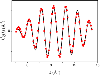
Figure 4: Experimental (full black line) and simulated (red squares) EXAFS $k^{3}\chi(k)$ signal at Se K edge for a-Se_0.80S_0.20.

It is important to note that, concerning the XRD structure factor ${\mathcal{S}}(K)$, the main contribution to it comes from Se-Se pairs. For instance, at $K=1$ Å^-1, the coefficients $w_{ij}(K)$, given by eq. 3, are $w_{\text{Se-Se}}=0.804$, $w_{\text{Se-S}}=0.185$ and $w_{\text{S-S}}=0.0107$. Thus, the contribution of ${\mathcal{S}}_{\text{Se-Se}}(K)$ to ${\mathcal{S}}(K)$ is about 80.4% (see eq. 2), while the contribution of ${\mathcal{S}}_{\text{Se-S}}(K)$ is around 18.5%, and the remaining 1.1% is associated to ${\mathcal{S}}_{\text{S-S}}(K)$. This fact makes the error bars of the structural parameters related to Se-Se pairs much smaller than those associated with Se-S pairs and we have only estimates concerning S-S pairs. Fig. 5 shows the $g_{ij}(r)$ functions obtained from the RMC simulations for a-Se_0.80S_0.20 (thick lines) and for a-Se_0.90S_0.10 (thin lines), for comparison.

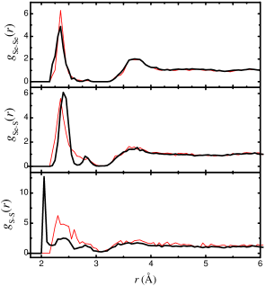
Figure 5: $g_{\text{Se-Se}}(r)$, $g_{\text{Se-S}}(r)$ and $g_{\text{S-S}}(r)$ functions obtained from the RMC simulations for a-Se_0.80S_0.20 (thick black lines) and for a-Se_0.90S_0.10 (thin red lines) for comparison.

Fig. 5 shows interesting features. First, considering the $g_{\text{Se-Se}}(r)$ function, its maximum corresponding to the Se-Se first neighbors is located at $r^{\text{Se-Se}}_{max}=2.35$ Å, at the same place where it is found in a-Se_0.90S_0.10. However, the Se-Se average interatomic distance is a little longer, being $\langle r^{\text{Se-Se}}\rangle=2.37$ Å. In addition, there is a decrease in the Se-Se average coordination number, from $\langle N^{\text{Se-Se}}\rangle=1.8$ in a-Se_0.90S_0.10 to $\langle N^{\text{Se-Se}}\rangle=1.6$ in a-Se_0.80S_0.20, as we expected. To obtain these values we considered the range between 1.90 Å and 3.00 Å in the calculations.

Considering now the $g_{\text{Se-S}}(r)$ function, the first point to note is the appearence of a small second shell close to the first peak in $g_{\text{Se-S}}(r)$. This second shell could be already present in a-Se_0.90S_0.10 but it was not well defined there. The use of EXAFS data in the RMC simulations for a-Se_0.80S_0.20 resolved it better and we could calculate the average coordination number associated with both shells. Here we considered that the Se-S first shell is formed by these two subshells, so the Se-S average coordination number for first neighbors is the sum of the values found for each subshell. The first subshell corresponds to $\langle N^{\text{Se-S}}_{1}\rangle=0.51$, and the second subshell contributes with $\langle N^{\text{Se-S}}_{2}\rangle=0.08$ to the total value $\langle N^{\text{Se-S}}\rangle=0.59$, which is almost twice larger than the value obtained for a-Se_0.90S_0.10. Even if we consider only the first Se-S subshell, the average coordination number is larger than that of a-Se_0.90S_0.10 by 67%. The total Se average coordination number, given by $\langle N^{\text{Se}}\rangle=\langle N^{\text{Se-Se}}\rangle+\langle N^{\text{Se-S}}\rangle$, is then $\langle N^{\text{Se}}\rangle=2.2$, larger than the value given by Heiba et al. Heiba ($\langle N^{\text{Se}}\rangle=2$) and by Shama Shama ($\langle N^{\text{Se}}\rangle=2.1$).

The second point about $g_{\text{Se-S}}(r)$ is that the position of the first shell increased. The first Se-S subshell is found at $\langle r^{\text{Se-S}}_{1}\rangle=2.42$ Å, and its maximum is at $r^{\text{Se-S}}_{1,max}=2.40$ Å, which is larger than the value found for a-Se_0.90S_0.10 in Ref. klese90s10 for the same shell ($\langle r^{\text{Se-S}}\rangle=2.34$ Å). For the second subshell we found $\langle r^{\text{Se-S}}_{2}\rangle=2.83$ Å and $r^{\text{Se-S}}_{2,max}=2.80$ Å. Thus, considering both subshells we have $\langle r^{\text{Se-S}}\rangle=2.48$ Å. The ranges used for the average calculations were [1.90–2.66] for the first subshell and [2.66–3.05] for the second.

Finally, we can now discuss the $g_{\text{S-S}}(r)$ function. As we already pointed out, the contribution of S-S pairs to the XRD ${\mathcal{S}}(K)$ is very small, so we are mainly interested on its qualitative features. As fig. 5 shows, one hypothesis is to think of the S-S first shell as formed by three subshells and to find the partial average coordination numbers and interatomic distances for each subshell. However, in this case we followed a different procedure, considering the first shell as ranging from 2.00 Å to 3.10 Å and, with this choice, we found $\langle N^{\text{S-S}}\rangle=1.2$ and $\langle r^{\text{S-S}}\rangle=2.27$ Å. There is a clear increase in the S-S average coordination number as the sulphur concentration goes from $x=0.10$ in a-Se_0.90S_0.10 to $x=0.20$ in a-Se_0.80S_0.20. It should be noted that these sulphur atoms belong to the amorphous Se_0.80S_0.20 phase, and the presence of a crystalline phase of sulphur can be ruled out since Raman results presented at fig. 2 show the disappearance of the c-S Raman modes in both a-Se_0.90S_0.10 and a-Se_0.80S_0.20. All results above are summarized on table 2.

Table 2: Structural parameters obtained for a-Se_0.80S_0.20 from RMC simulations.

Bond type	Se-Se	Se-S	S-S
$\langle N\rangle$	$1.6\pm 0.1$	$0.59\pm 0.1$	$1.2\pm 0.2$
$\langle r\rangle$ (Å)	$2.37\pm 0.05$	$2.48\pm 0.07$	$2.27\pm 0.15$

² There are two subshells with $\langle N^{\text{Se-S}}_{1}\rangle=0.51$ and $\langle N^{\text{Se-S}}_{2}\rangle=0.08$, respectively.

² There are two subshells at $\langle r^{\text{Se-S}}_{1}\rangle=2.42$ Å and $\langle r^{\text{Se-S}}_{2}\rangle=2.83$ Å, respectively.

4.4 Optical Gap Energy Determination

In addition to the structural and vibrational properties of a-Se_0.80S_0.20, we also calculated its optical gap energy. Fig. 6 shows the absorbance obtained for this alloy. The absorption edge appears around 610 – 670 nm. As discussed on sec. 3.2, we used two methods to estimate the optical gap. First, we made extrapolations of the baseline and the absorption edge Boldish , which are shown in fig. 6 (dashed lines). This procedure furnished a gap located at 674.4 nm, indicated in the figure by the vertical dotted line, corresponding to the value $E_{g}=1.84$ eV.

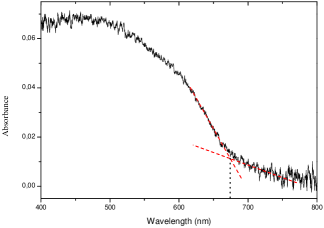
Figure 6: Absorption spectrum determined for a-Se_0.80S_0.20 and extrapolations to the baseline and to the absorption edge (dashed lines). The vertical dotted line indicates the crossing of both lines, which is the estimative of the band gap.

We also used the McLean procedure McLean to obtain the optical gap. Fig 7 shows the best fit achieved using eq. 9. We found a direct band gap ($n=2$) at $E_{g}=1.87$ eV for a-Se_0.80S_0.20, indicating and increase in the gap energy with the increase in the sulphur concentration, since the value found for a-Se_0.90S_0.10 klese90s10 was $E_{g}=1.81$ eV. For a comparison, Rafea and Farag Rafea obtained, for an amorphous Se_0.80S_0.20 thin film, $E_{g}=1.96$ eV.

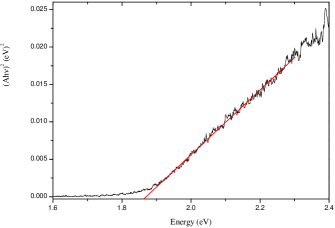
Figure 7: Plot of $(Ah\nu)^{2}\times h\nu$ and linear fit for a-Se_0.80S_0.20 to obtain the optical gap energy.

5 Conclusion

The amorphous Se_0.80S_0.20 alloy was prepared by MA and its local atomic structure investigated. The main conclusions of this study are:

1. The average number of Se-S pairs in the alloy increases as the sulphur concentration is raised from $x=0.10$ in a-Se_0.90S_0.10 to $x=0.20$ in a-Se_0.80S_0.20, showing that alloying occurs in an atomic level. Fukunaga et al. Fukunaga2 stated that there was only a mixing of Se chains and S rings in Se-S amorphous alloys, but Raman results and RMC simulations refuse this assumption. It is interesting to note that, although the Se-Se average coordination number decreased, the average total coordination number for Se atoms increases and is larger than 2. In addition, the S-S average coordination number also increases as $x$ increases.

2. The density of the alloy seems to be independent of the sulphur concentration, at least for a-Se_0.90S_0.10 and a-Se_0.80S_0.20.

3. The optical gap of the alloy is also a function of the sulphur concentration, and it increases as the S content is increased, going from $E_{g}=1.81$ eV for a-Se_0.90S_0.10 to $E_{g}=1.87$ eV for a-Se_0.80S_0.20.

4. Concerning the simulations, the use of EXAFS data on RMC simulations besides XRD ${\mathcal{S}}(K)$ produced better resolved shells, and furnished more reliable structural data.

- (1) M. F. Kotkata, F. M. Ayad, and M. K. El-Mously. J. Non-Cryst. Solids, 33:13, 1979.
- (2) M. F. Kotkata, M. F. El-Fouly, A. Z. El-Behay, and L. A. El-Wahab. Mat. Sci. & Eng., 60:163, 1983.
- (3) E. A. Mahmoud. J. Thermal Analysis, 36:1481, 1990.
- (4) N. Musahwar, M. A. M. Khan, M. Husain, and M. Zulfequar. Physica B, 396:81, 2007.
- (5) M. A. Rafea and A. A. M. Farag. Chalc. Letters, 5:27, 2008.
- (6) A. T. Ward. J. of Phys. Chem., 72:4133, 1968.
- (7) M. F. Kotkata, S. A. Nouh, L. Farkas, and M. M. Radwan. J. Mat. Sci., 27:1785, 1992.
- (8) M. F. Kotkata, M. Füstoss-Wegner, L. Toth, G. Zental, and S. A. Nouh. J. Phys. D: Appl. Phys., 26:456, 1993.
- (9) Z. K. Heiba, M. B. El-Den, and K. El-Sayed. Pow. Diff., 17:1861, 2002.
- (10) A. A. Shama. Egypt. J. Solids, 28:25, 2005.
- (11) T. Fukunaga, S. Kajikawa, Y. Hokari, and U. Mizutani. J. Non-Cryst. Solids, 232-234:465, 1998.
- (12) C. Suryanarayana. Prog. Mat. Sci., 46:1, 2001.
- (13) K. D. Machado, D. F. Sanchez, G. A. Maciel, S. F. Brunatto, A. S. Mangrich, and S. F. Stolf. J. Phys.: Condens. Matter, 21:195406, 2009.
- (14) R. L. McGreevy. J. Phys.: Condens. Matter, 13:877, 2001.
- (15) O. Gereben, P. Jóvári, L. Temleitner, and L. Pusztai. J. Optoelec. Adv. Mat., 9:3021, 2007.
- (16) B. Ravel and M. Newville. J. Synchrotron Rad., 12:537, 2005.
- (17) H. F. Poulsen, J. Neuefeind, H.-B. Neumann, J. R. Schneider, and M. D Zeidler. J. Non-Cryst. Solids, 188:63, 1995.
- (18) T. E. Faber and J. M. Ziman. Philos. Mag., 11:153, 1965.
- (19) K. D. Machado, P. Jóvári, J. C. de Lima, A. A. M. Gasperini, S. M. Souza, C. E. Maurmann, R. G. Delaplane, and A. Wannberg. J. Phys.: Condens. Matter, 17:1703–1710, 2005.
- (20) P. Jóvári, I. Kaban, J. Steiner, B. Beuneu, A Schöps, and M. A. Webb. Phys. Rev. B, 77:035202, 2008.
- (21) C. Tengroth, J. Swenson, A. Isopo, and L. Borjesson. Phys. Rev. B, 64:224207, 2001.
- (22) E. W. Iparraguirre, J. Sietsma, and B. J. Thijsse. J. Non-Cryst. Solids, 156–158:969, 1993.
- (23) S. I. Boldish and W. B. White. Am. Miner., 83:865, 1998.
- (24) T. P. McLean. Prog. Semicond., 5:55, 1960.
- (25) F. Q. Guo and K. Lu. Phys. Rev. B, 57:10414, 1998.
- (26) K. D. Machado, J. C. de Lima, C. E. M. Campos, A. A. M. Gasperini, S. M. de Souza, C. E. Maurmann, T. A. Grandi, and P. S. Pizani. Sol. State Commun., 133:411, 2005.
- (27) C. E. M. Campos, J. C. de Lima, T. A. Grandi, K. D. Machado, and P. S. Pizani. Sol. State Commun., 126:611, 2003.
- (28) S. Sugai. Phys. Rev. B, 35:1345, 1987.
- (29) O. Gereben and L. Pusztai. Phys. Rev. B, 50:14136, 1994.